The Chandra High Energy Transmission Grating: Design,
Fabrication, Ground Calibration and Five Years in Flight
The MIT Faculty has made this article openly available.
Please share
how this access benefits you. Your story matters.
Citation
Canizares, Claude R. et al. “The Chandra High#Energy Transmission
Grating: Design, Fabrication, Ground Calibration, and 5 Years in
Flight.” Publications of the Astronomical Society of the Pacific
117.836 (2005): 1144–1171.
As Published
http://dx.doi.org/10.1086/432898
Publisher
University of Chicago Press, The
Version
Author's final manuscript
Citable link
http://hdl.handle.net/1721.1/71916
Terms of Use
Article is made available in accordance with the publisher's
policy and may be subject to US copyright law. Please refer to the
publisher's site for terms of use.
arXiv:astro-ph/0507035v1 1 Jul 2005
The Chandra High Energy Transmission Grating:
Design, Fabrication, Ground Calibration and Five Years in Flight
Claude R. Canizares, John E. Davis, Daniel Dewey, Kathryn A. Flanagan, Eugene B.
Galton, David P. Huenemoerder, Kazunori Ishibashi, Thomas H. Markert, Herman L.
Marshall, Michael McGuirk, Mark L. Schattenburg, Norbert S. Schulz, Henry I. Smith and
Michael Wise
crc@space.mit.edu
MIT Kavli Institute, Cambridge, MA 02139
ABSTRACT
Details of the design, fabrication, ground and flight calibration of the High Energy Trans-mission Grating, HETG, on the Chandra X-ray Observatory are presented after five years of flight experience. Specifics include the theory of phased transmission gratings as applied to the HETG, the Rowland design of the spectrometer, details of the grating fabrication techniques, and the results of ground testing and calibration of the HETG. For nearly six years the HETG has operated essentially as designed, although it has presented some subtle flight calibration effects.
Subject headings: space vehicles: instruments – instrumentation: spectrographs – X-rays: general – methods: laboratory – techniques: spectroscopic
1. Introduction
The Chandra X-ray Observatory (Weisskopf, Tananbaum, van Speybroeck, & O’Dell 2000), for-merly the Advanced X-ray Astrophysics Facility, AXAF, was launched on July 23, 1999, and for five years has been realizing its promise to open new domains in high resolution X-ray imaging and spectroscopy of celestial sources (Weisskopf et al. 2004, 2002). The High Energy Transmis-sion Grating, HETG (Canizares et al. 2000), is one of two objective transmission gratings on Chan-dra; the Low Energy Transmission Grating, LETG (Brinkman et al. 2000), is of a similar design but optimized for energies less than 1 keV. When the HETG is used with the Chandra mirror and a fo-cal plane imager, the resulting High Energy Trans-mission Grating Spectrometer, HETGS, provides spectral resolving powers of up to 1000 over the range 0.4-8 keV (1.5-30 ˚A) for point and moder-ately extended sources. Through year 2004, the HETGS has been used in 422 observations cov-ering the full range of astrophysical sources and totaling 20 Ms, or 17 % of Chandra observing
time. Up-to-date information on Chandra and the HETG is available from the Chandra X-ray-Center (CXC 2004). This paper summarizes the design, fabrication, ground and flight calibration of the HETG.
The High Energy Transmission Grating, HETG (Canizares, Schattenburg, & Smith 1985; Canizares et al. 1987; Markert 1990; Schattenburg et al. 1991; Markert et al. 1994), is a passive array of 336 diffraction grating facets each about 2.5 cm square. Each facet is a periodic nano-structure consisting of finely spaced parallel gold bars sup-ported on a thin plastic membrane. The facets are mounted on a precision HETG Element Sup-port Structure, HESS, which in turn is mounted on a hinged yoke just behind the High Resolu-tion Mirror Assembly, HRMA (van Speybroeck et al. 1997). A telemetry command to Chandra acti-vates a motor drive that inserts HETG into the op-tical path just behind the HRMA, approximately 8.6 m from the focal plane, shown schematically in Figure 1. The lower portion of this figure shows a schematic of the Advanced CCD Imaging
Spec-trometer (Garmire 1999) spectroscopy detector, ACIS-S, with the HETG’s shallow “X” dispersion pattern indicated. This pattern arises from the use of two types of grating facets in the HETG, with dispersion axes offset by 10 deg so that the corresponding spectra are spatially distinct on the detector.
The choice (and complexity) of using two types of grating facets resulted from our desire to achieve optimum performance in both diffraction effi-ciency and spectral resolution over the factor-of-20 energy range from 0.4 to 8 keV. These facets are the heart of the HETG and are schematically shown in Figure 2 with their properties given in Table 1. One type, the Medium Energy Grating (MEG), has spatial period, bar thickness, and sup-port membrane thickness optimized for the lower portion of the energy range. These MEG facets are mounted on the two outer rings of the HESS so that they intercept rays from the outer two mir-ror shells of the HRMA, which account for ∼65% of the total HRMA effective area below 2 keV. The second facet type, the High Energy Grating (HEG), has finer period for higher dispersion and thicker bars to perform better at higher energies. The HEG array intercepts rays from the two inner HRMA shells, which have most of the area above ∼5 keV.
When the HRMA’s converging X-rays pass through the transmission grating assembly they are diffracted in one dimension by an angle β given by the grating equation at normal incidence,
sin β = mλ/p, (1)
where m is the integer order number, λ is the photon wavelength, 1 p is the spatial period
of the grating lines, and β is the dispersion an-gle. A “normal” undispersed image is formed by the zeroth-order events, m = 0, while the higher orders form overlapping dispersed spectra that
1 Wavelength bins are “natural” for a dispersive spec-trometer (e.g., the dispersion and spectral resolution (∆λ) are nearly constant with λ) and wavelength is commonly used in the high-resolution X-ray spectroscopy commu-nity. However, since photon energy has been commonly used in high-energy X-ray astrophysics (as is appropriate for non-dispersive spectrometers like proportional counters and CCDs), we use either energy or wavelength values in-terchangeably depending on the context. The values are related through: E × λ = 12.3985 keV˚A.
stretch on either side of the zeroth-order image. By design the first orders, m = ±1, dominate. Higher orders are also present however the ACIS itself has moderate energy resolution sufficient to allow the separation of the overlapping diffracted orders.
As with other spectrometers, the overall per-formance of the HETGS can be characterized by the combination of the effective area encoded in an Auxiliary Response Function, ARF (Davis 2001a), and a line response function, LRF, encoded as a Response Matrix Function, RMF. For this grat-ing system the LRF describes the spatial distri-bution of monochromatic X-rays along the disper-sion direction; a simple measure of the LRF is the full width at half maximum (FWHM), ∆λFWHM,
expressed in dimensionless form as the resolving
power, λ/∆λFWHM ≡ E/∆EFWHM. With the
HRMA’s high angular resolution (better than 1 arc sec), the HETG’s high dispersion (as high as 100 arc seconds/˚A), and the small, stable pixel size (24 µm or ∼ 0.5 arc sec) of ACIS-S, the HETGS achieves spectral resolving powers up to E/∆E ≈ 1000.
The following sections present details of the key ingredients and papers related to the design of the HETGS, the fabrication and test of the individ-ual HETG grating facets, and the results of full-up ground calibration of the flight HETG. The final section demonstrates the HETGS flight per-formance and discusses the calibration status of the instrument after five years of flight operation.
2. HETG Design
2.1. Theory of Phased Transmission
Grat-ings
Obtaining high throughput requires that X-rays are dispersed into the m = ±1 orders with high diffraction efficiency; this is largely determined by the micro-properties of the MEG and HEG grating bars and support membranes. Both the MEG and HEG facets are designed to operate as “phased” transmission gratings to achieve enhanced diffrac-tion efficiency over a significant pordiffrac-tion of the en-ergy range for which they are optimized (Schnop-per et al. 1977). A conventional transmission grat-ing with opaque gratgrat-ing bars achieves a maximum efficiency in each ±1st order of 10%, for the case
pp. 401-414). In contrast, the grating bars of the MEG and HEG are partially transparent – X-rays passing through the bars are attenuated and also phase-shifted, depending on the imaginary and real parts, respectively, of the index of refraction at the given λ. Ideally, the grating material and thickness can be selected to give low attenuation and a phase-shift of ≈ π radians at the desired en-ergy (Schattenburg 1984). This causes the radia-tion that passes through the bars to destructively interfere with the radiation that passes through the gaps when in zeroth order (where the rele-vant path-lengths are equal) reducing the amount of undiffracted (zeroth-order) radiation and, con-versely, enhancing the diffracted-orders efficiency. In practice, this optimal phase interference can only be obtained over a narrow wavelength band, as seen in Figure 3, because of the rapid depen-dence of the index of refraction on wavelength. Initial designs based on these considerations sug-gested using gold for the HEGs and silver for the MEGs; in the end, fabrication considerations lead to selecting gold for both grating types and opti-mizing the bar thicknesses of the MEG and HEG gratings.
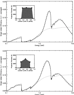
Because the grating bars are not opaque, the diffraction efficiency also depends on the cross-sectional shape of the bars, and this shape must be determined and incorporated into the model of the instrument performance. The effect of phase shifting is shown in Figure 3 where the dotted line represents the single-side 1st order diffraction
effi-ciency (i.e., one-half the total 1storder diffraction
efficiency) for a non-phased opaque grating and the dashed and solid lines are from models which include the phase-shifting effects. For the opaque case (dotted), the diffraction efficiency of the grat-ing bars is constant with energy; the variations seen in Figure 3 result from also including the ab-sorption by the support membrane and the plating base, the thin base layers shown in Figure 2, whose thicknesses are given in Table 1. These layers are nearly uniform over the grating and therefore only absorb X-rays.
The phased HEG and MEG gratings achieve higher efficiencies than opaque gratings over a sig-nificant portion of the energy band. The struc-ture in the HEG and MEG efficiencies is caused by structure in the index of refraction of gold, i.e., the M edges around 2 keV. The efficiency falls at high
energy as the bars become transparent and intro-duce less phase shift to the X-rays, falling below the opaque value at an energy depending on their thickness. The general formula for the efficiency of a periodic transmission grating, using Kirchhoff diffraction theory with the Fraunhofer approxima-tion is (Born & Wolf 1980, pp. 401-414):
gm(λ) = 1 p2× Z p 0 dx eik(ν(k)−1)z(xp)+i2πm x p 2 (2) where gm is the efficiency in the mth order, k is
the wavenumber (2π/λ), ν(k) is the complex in-dex of refraction often expressed in real and imag-inary parts (or optical constants) as ν(k) − 1 = −(δ(k) − iβ(k)), p is the grating period, and z(ξ) is the grating path-length function of the normal-ized coordinate ξ = x/p. The path-length function z(ξ) may be thought of as the projected thickness of the grating bar versus location along the direc-tion of periodicity; at normal incidence it is simply the grating bar cross-section.
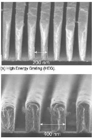
The path-length function z(ξ) can be reduced to a finite number of parameters. For example, if a rectangular bar shape is assumed, then z can be computed with two parameters, a bar width and a bar thickness (or height.) Adding an addi-tional parameter, Fischbach et al. (1988) reported on the theory and measurements of tilted rect-angular gratings which yields a trapezoidal path-length function for small incident angles. Our data are fit adequately for performance estimates if a simple rectangular grating bar shape is assumed (Schnopper et al. 1977; Nelson et al. 1994). How-ever, modeling the measured first-order efficien-cies to ∼1 % requires a more detailed path-length function. This is not surprising given the evidence from electron microscope photographs (Figure 9) that the bar shapes for the HETG gratings are not simple rectangles.
We found from laboratory measurements (see below) that sufficient accuracy could be achieved by modeling the grating bar shape in a piece-wise linear fashion. We parameterize the shape by specifying a set of vertices, e.g., as shown in the insets of Figure 3, by their normalized locations, ξj, and thicknesses, z(ξj); the end-point vertices
are fixed at (0,0) and (1,0). We have found in our modeling that 5 variable vertices are sufficient to accurately model these gratings in 0th, 1st and
2nd orders and yet not introduce redundant
pa-rameters. Finally, this multi-vertex path-length function also lends itself to simple calculation as presented in Appendix A.
Note that this multi-vertex model allows an asymmetric (effective) bar shape which generally leads to unequal plus and minus diffraction orders, as in the case of a blazed transmission grating (Michette & Buckley 1993) or as arises when a trapezoidal grating is used at off-normal (“tilted”) incidence. Hence, this multi-vertex model can be a useful extension of the symmetric, multi-step scheme formulation in Hettrick et al. (2004). For the HETG gratings this asymmetric case arises primarily when the roughly trapezoidal HEG grat-ings were tested at non-normal incidence, produc-ing an asymmetry of up to 30 % per degree of tilt. However, the asymmetry is linear for small tilt angles from the normal and so the sum of the plus and minus order efficiencies remains nearly constant.
2.2. Synchrotron Measurements and
Op-tical Constants
We used high intensity X-ray beams at sev-eral synchrotron radiation facilities for sevsev-eral pur-poses: (i) to measure the optical constants and absorption edge structure of the grating materials and supporting polyimide membranes; (ii) to make absolute efficiency measurements of several grat-ings to validate and constrain our grating perfor-mance model and provide estimates of its intrinsic uncertainties; (iii) to calibrate several gratings for use as transfer standards in our in-house calibra-tion; and (iv) to measure the efficiencies of several gratings also calibrated in-house to assess uncer-tainties; see Flanagan et al. (1996, 2000). Syn-chrotron radiation tests were performed at four facilities over several years.
A first set of measurements were made at the National Synchrotron Light Source (NSLS) at Brookhaven National Laboratory (BNL) piggy-backing on equipment and expertise Graessle et al. (1996) developed to support the determina-tion of the reflectivity properties of the HRMA coating. The general configuration of these tests is indicated in Figure 4; key ingredients are: an input of bright, monochromatic X-rays from the beam line, a beam monitoring detector which is inserted frequently to normalize the beam
inten-sity, a detector fitted with a narrow slit (0.002 and 0.008 inches were used) that could be rotated to intercept radiation at a desired diffraction an-gle, and the grating itself which could be rotated (“tilted”) about the vertical (grating bar) axis and also removed for detector cross-calibration. Data sets were taken automatically with one or more of the controlled parameters varied: monochromator energy scan, diffraction angle (order) scan, and a grating tilt scan.
Initial modeling based on a rectangular grating bar model and using the optical constants, δ and β, obtained from the scattering factors (f1, f2)
published by Henke, Gullikson, & Davis (1993) indicated significant disagreement with the Henke values for the gold optical constants (Nelson et al. 1994; Markert et al. 1995). The most notice-able feature was that the energies of the gold M absorption edges were shifted from the tabulated amounts by as much as 40 eV, a result obtained earlier by Blake et al. (1993) from reflection stud-ies of gold mirrors. In an effort to determine more accurate optical constants, the transmission of a gold foil was measured over the range 2.03– 6.04 keV, and the values of β and δ were revised (Nelson et al. 1994). The widely used Henke tables were modified in 1996 to reflect these results.
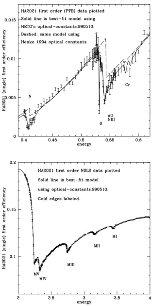
Subsequent tests on gratings explored bar shape, tilt and asymmetry (Markert et al. 1995), and tests at the radiometry laboratory of the Physikalish-Technische Bundesanstalt (PTB) be-low 2 keV identified the need to accurately model the edge structures of the polyimide support mem-brane to improve the overall fit (Flanagan et al. 1996). The analysis of the tests of gold and poly-imide membranes at PTB in October 1995 is detailed in Flanagan et al. (2000). In addition, cross-checks of the revised gold constants (above 2 keV) and polyimide were performed in August and November 1996 and have confirmed these lat-est revisions.
As a consequence of these analyses, our model now includes revised gold optical constants over the full energy range appropriate to the HETG, and detailed structure for absorption edges of polyimide, C22H10O4N2, and Cr. An example of
the agreement between measured and modeled ef-ficiencies is shown in Figure 5.
2.3. The Faceted Rowland Design
The HETGS optical design is based on an ex-tension of the simple Rowland spectrometer de-sign in which the gratings and detector are located on opposite sides of an imaginary Rowland circle (Born & Wolf 1980). The Rowland configuration maintains the telescope focal properties in the dis-persion direction for a large range of diffraction an-gle, β, thereby minimizing aberrations. A detailed discussion of the physics of Rowland spectrome-ters, i.e., applying Fermat’s principle (Schroeder 1987) to evaluate aberrations of the faceted grat-ing design, is given by Beuermann, Br¨auniger, & Tr¨umper (1978). What follows is a simplified, ray-based description of the basic design.
The “Top View” of Figure 6 shows the plane of dispersion (the (x′, y′) plane), as viewed along
the cross-dispersion direction, z′. The diffraction
angle is β, as defined by Equation 1; note that the facet surfaces are normal to the incoming, central X-rays and are thus not tangent to the Rowland circle. Through the geometric properties of the circle, rays diffracted from gratings located along the Rowland circle will all converge at the same diffracted point on the Rowland circle. The dotted lines represent zeroth-order (m = 0, β = 0) rays and the solid lines a set of diffracted order (m > 0, β > 0) rays.
The bottom panel, “Side View”, gives a view along the dispersion direction, y′, at rays from a
set of grating facets located in the the (x′, y′) plane
(the same three facets in the “Top View” now seen in projection, shown in light shading) as well as additional grating facets (darker facets) located above (or equivalently below) the (x′, y′) plane.
Each arc of additional facets is located on another Rowland circle obtained by rotating the circle in the Top View about the right-most line segment: the tangent to the Rowland circle that is parallel to the dispersion direction and passes through the zeroth order focal point. The surface described by this rotation is the Rowland torus. All grating facets with centers located on this Rowland torus and with surfaces normal to the converging rays (dotted lines) will focus their diffracted orders on a common arc on the Rowland circle in the (x′, y′)
plane. Since the Rowland diameter is the same for all grating facets, and the zero order focus coin-cides for all facets, the mth diffracted order from
each facet is focused at the same angle β, at the same place on the Rowland circle. That is, best focus for the dispersion direction projection occurs along the inner surface of the Rowland torus.
Together, these constructions show the astig-matic nature of the dispersed image: the rays come to a focus in the dispersion direction, the Rowland focus, at a different location from their focus in the cross-dispersion direction, the Imag-ing focus. This is demonstrated in the ray-trace example of Figure 7.
In order to maintain the best spectroscopic focus the detector surface must conform to or approximate this Rowland curvature so that diffracted images are focused and sharp in the dispersion direction, and elongated in the cross-dispersion direction. The offset of the Rowland circle from the tangent at the zeroth order focus is
∆XRowland= β2XRS (3)
where XRS is the Rowland spacing, the diameter
of the Rowland circle.
At the Rowland focus, e.g., the dx = 0 case in Figure 7, the image is elongated (blurred) in the cross-dispersion direction, z′, due to the
astig-matic nature of the focus and has a peak-to-peak value given by:
∆zastig′ =
2R0
XRS
∆XRowland (4)
Here R0is the radius of the ring of gratings around
the optical axis as defined in Figure 6. The width of the image in the dispersion direction, y′, is given
by a term proportional to the size of the (planar) grating facets which tile the Rowland torus. The peak-to-peak value of this “finite-facet size” blur is given by: ∆y′ ff = L XRS (R0β + ∆XRowland 2 ) (5)
where L is the length of a side of the square grat-ing facet. This blur sets the fundamental resolvgrat-ing power limit for the Rowland design with finite-sized facets. For the HETGS design this contri-bution is much smaller than the ACIS pixel size, see the dx = 0 case of Figure 7, and is negligi-ble compared to the terms in the resolving power error budget of Appendix B.
3. HETG Fabrication, Test, and Assembly
3.1. Facet Fabrication
The 144 HEG and 192 MEG grating facets are the key components of the HETG and presented major technical challenges: to create facets with nanometer scale periods, nearly rectangular bar shape, nearly equal bar and gap widths, and suf-ficient bar depth to achieve high diffraction effi-ciencies, and with a high degree of uniformity in all these properties within each facet and among hundreds of facets. The facets must also be suf-ficiently robust to withstand the vibrational and acoustic rigors of space launch without altering their properties, much less being destroyed.
The HETG grating facets were fabricated, one at a time, in an elaborate, multi-step process em-ploying techniques adapted from those used to fab-ricate large-scale integrated circuits. Development work was initiated in the Nano Structures Labora-tory and refinement of these processes took place over nearly two decades with final flight produc-tion in the Space Nanotechnology Laboratory of the (then) MIT Center for Space Research.
Each facet was fabricated on a silicon wafer, which was used as a substrate but did not form any part of the final facet. In brief, the process in-volved depositing the appropriate material layers on the wafer, imprinting the period on the outer-most layer using UV laser interference, transfer-ring that periodic pattern to the necessary depth, thereby creating a mold with the complement of the desired grating geometry, filling the mold with gold using electroplating, stripping away the mold material, etching away a portion of the Si sub-strate, aligning and attaching a frame and then separating the finished facet from the silicon wafer. A highly simplified depiction of these steps is given in Fig. 8 and described below. More complete de-tails of the fabrication process are available else-where (Schattenburg, Aucoin, Fleming, Plotnik, Porter, & Smith 1994; Schattenburg 2001).
The first step, Fig. 8a, is to coat 100 mm-diameter silicon wafers with six layers of polymer, metal, and dielectric, comprising either 0.5 (MEG) or 1.0 (HEG) microns of polyimide (which will later form the grating support membrane), 5 nm of chromium (for adhesion) and 20 nm of gold which serve as the plating base, ≈500 nm of
anti-reflection coating (ARC) polymer, 15 nm of Ta2O5
interlayer (IL), and 200 nm of UV imaging pho-topolymer (resist).
The second step, Fig. 8b, is to expose the re-sist layer with the desired periodic pattern of the final grating using interference lithography at a wavelength of 351.1 nm. Two nearly spherical, monochromatic wavefronts interfere to define the grating pattern period; the radii of the spheri-cal wavefronts are sufficiently large to reduce the inherent period variation across the sample to less than 50 ppm rms. A high degree of period repeatability is required from the hardware be-cause a unique exposure is used for each grat-ing facet of the HETG. Prior to each exposure, the Moire´e pattern between the UV interference standing waves and a stable reference grating fab-ricated on silicon was used to lock the interfer-ometer period. A secondary interferinterfer-ometer and active control are used to ensure that the interfer-ence pattern is stable over the approximately one minute exposure time. The interlayer, ARC, and resist layers form an optically-matched stack de-signed to minimize the formation of planar stand-ing waves normal to the surface, which would com-promise contrast and linewidth control (Schatten-burg, Aucoin, & Fleming 1995).
In the third step, Fig. 8c, the resist pattern is transferred into the interlayer using CF4
reactive-ion plasma etching (RIE). In the fourth step, Fig. 8d, the IL pattern is transferred into the ARC using O2 RIE. The RIE steps are designed
to achieve highly directional vertical etching with minimal undercut.
The fifth step, Fig. 8e, is to electroplate the ARC mold with low-stress gold, which builds up from the Cr/Au plating base layer. The sixth step, Fig. 8f, is to strip the ARC/IL plating mould using hydrofluoric (HF) acid etch, and plasma etching with CF4 and O2. At this point the gold grating
bars are complete; Figure 9 shows electron micro-graphs of cleaved cross-sections of the gratings.
In the last step, Fig. 8g, a circular portion of the Si wafer under the grating and membrane is etched through from the backside in HF/HNO3 acid us-ing a spin etch process that keeps the acid from attacking the materials on the front side (Schat-tenburg et al. 1995). The membrane, supported by the remaining ring of un-etched Si wafer, is then aligned to an angular tolerance of ≤ 0.5
de-gree and bonded to a flight “frame” using a two-part, low-outgassing epoxy. Once cured, the ex-cess membrane and Si ring is cut away from the frame with a scalpel. The frames are custom-made of black chrome plated Invar 36, machined to tight tolerances, and the membrane bonding faces were hand lapped to remove burrs and ensure a flat, smooth surface during bonding. Use of Invar re-duces any grating period variations which might be caused by thermal variation of the HETG en-vironment between stowed and in-use positions on Chandra. Likewise, the frame design has a single mounting hole to reduce the effect of mounting stresses on the facet period. Each completed facet was mounted in a non-flight “holder” to allow for ease in storing, handling, and testing; a schematic of holder and facet is shown in Figure 10.
After years of preparation, we fabricated 245 HEG and 265 MEG gratings in 21 lots over a pe-riod of 16 months; tests on the individual facets, next section, were used to select the elite set of 336 flight grating facets. As a postscript to the fabrication of the Chandra HETG facets, we note that we have since extended our technol-ogy (Schattenburg 2001) to fabricate gratings with finer periods (Savas et al. 1996), mesh-supported “free-standing” gratings for UV/EUV and atom beam diffraction and filtering (Beek et al. 1998), and super-smooth reflection gratings (Franke et al. 1997).
3.2. Facet Laboratory Tests & Calibration The completed HETG facets were put through a set of laboratory tests to characterize their qual-ity and performance and to enable selection of an optimal complement of flight gratings. Each facet went through a sequence of tests: i) Visual Inspec-tion, ii) Laser Reflection (LR) Test 1, iii) Acous-tic Exposure, iv) LR Test 2, v) Thermal Cycling, vi) LR Test 3, and finally vii) X-ray Testing. As noted, to reduce direct handling each fabricated facet was mounted to its own aluminum holder, the facet-level test equipment was designed to in-terface to the holder.
The laser reflection, LR, test (Dewey, Humphries, McLean, & Moschella 1994) uses optical diffrac-tion of a laser beam (HeNe 633nm for MEG, HeCd 325 nm for HEG) from the grating surface to mea-sure period and period variations of each facet. As shown in Figure 10 the laser beam is incident
on the grating under test at an off-normal an-gle. A specularly reflected beam and a first-order diffracted beam emerge from the illuminated re-gion of the grating. These beams are focused with simple, long-focal length (≈500 mm) lenses onto commercial CCDs. Under computer control the grating is moved so that a raster of over 100 regions is illuminated and the centroids of the re-flected and diffracted beams in the CCD imagers are measured and recorded. Changes in the four CCD spot coordinates, XRefl, YRefl, XDiff, YDiff,
are linearly related to changes in four local grat-ing properties: the gratgrat-ing surface tilt and tip, the grating period and the grating line orientation (roll.) These measurements are referenced to grat-ings (HEG and MEG) on silicon substrates per-manently mounted in the system and measured before and after each raster scan set. The LR data files are used to determine for each grating facet a mean period p and an rms period varia-tion dp/p as well as contours of period variavaria-tion across the facet. The flight grating sets were then selected to achieve minimal overall period varia-tion for the complete HEG and MEG arrays, 106 and 127 ppm rms, respectively. The ability of the LR apparatus to measure absolute period was calibrated using samples on silicon measured inde-pendently at the National Institute for Standards and Technology. The average periods of the grat-ing sets as determined from the LR measurements are given in Table 1, Laboratory Parameters.
The diffraction efficiency (Dewey, Humphries, McLean, & Moschella 1994) of each facet was mea-sured using the X-Ray Grating Evaluation Facil-ity, X-GEF, consisting of a laboratory electron-impact X-ray source, a collimating slit and grating assembly, and two detectors (a position sensitive proportional counter and a solid state detector) in a 17 m long vacuum system. Facet tests were con-ducted at a rate of 2 gratings per day. The zeroth, plus and minus first and second order efficiencies were measured for five swath-like regions on each facet and at up to six energies, Cu-L 0.930 keV, Mg-K 1.254 keV, Al-K 1.486 keV, Mo-L 2.293 keV, Ti-K 4.511 keV, and Fe-K 6.400 keV. Two facets, which had been tested at synchrotron facilities (Markert et al. 1995), served as absolute efficiency references. The measured monochromatic efficien-cies were fit with our multi-vertex efficiency model (Flanagan, Dewey, & Bordzol 1995), an example
model fit to X-GEF measured points is shown in Figure 11. These measurements and models al-lowed us to select the highest efficiency gratings for the flight HEG and MEG sets as well as to predict the overall grating-set efficiencies, Section 4.2.
The HETG flight-candidate gratings were X-GEF tested from mid-1995 through September of 1996 at a typical rate of two per day. A small set of non-flight gratings were retained in a labora-tory vacuum and their diffraction efficiencies were measured with X-GEF at seven epochs from late 1996 to February 2003. These “vacuum storage gratings” showed no evolution in their diffraction properties giving us an expectation of stability for the HETG efficiency calibration.
3.3. HETG Assembly
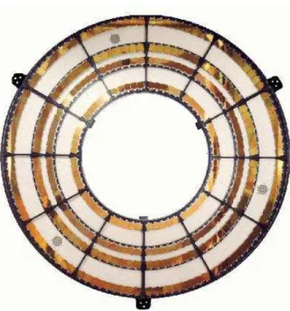
The flight HETG came into being when the selected 336 flight grating facets were mounted to the HETG Element Support Structure, HESS. The HESS was numerically machined from a single plate of aluminum ≈ 4 cm thick (Pak & McGuirk 1994; Markert et al. 1994) to create a spoke-and-ring structure with mounting surfaces and holes for the facets that conformed to the Rowland torus design with a diameter given in Table 1. The HESS mechanical design using tapered ≈ 6 mm thick spokes achieves the objectives of: a low weight, an accurate positioning of the facets, and the ability to withstand the high-g launch vibra-tion environment. The flight HETG is shown in Figure 12 where the HESS is black and the facet surfaces are gold; its outer diameter is 1.1 m and three attachment points provide for its mounting to one of the two Chandra telescope grating in-sertion mechanism yokes. The completed flight HETG weighs 10.41 kg of which 8.88 kg is due to the HESS structure, 1.21 kg for the grating ele-ments, and 0.32 kg for the the element-to-HESS mounting hardware. The “active ingredient” of the HETG, the gold grating bars, weighs a mea-ger 1.14 mg.
The single-screw mounting scheme used to at-tached the facets to the HESS adequately fixes all degrees of freedom of the facet except for rotation around the screw axis, i.e., the “roll” angle of the facet. The roll angle was aligned using the ability of the grating to polarize transmitted light which has a wavelength longer than the grating period. A schematic of our setup, based on the
polariza-tion alignment technique of Anderson, Levine, & Schattenburg (1988), is shown in Figure 13. Light from the HeNe laser passes through a photo-elastic modulator at a 45 degree angle. The emerging beam can be viewed as having two linearly polar-ized components at right angles with a time depen-dent relative phase varying as sin(ωt). Ignoring any effect of the polyimide on the light, the po-larizing grating bars transmit only the projection of these components that is perpendicular to the bars. For a non-zero θg some fraction of each of
the modulator-axes components is transmitted re-sulting in interference and an intensity signal at 2ω proportional to θg. This measurement setup was
used along with appropriate manipulation fixtur-ing to set each facet to its desired roll orientation (differing by ≈ 10 degrees between HEG and MEG facets) with, in general, an accuracy better than 1 arc minute.
When all facets were aligned and the alignment re-checked they were then epoxied to the HESS. The flight HETG was then subjected to a random vibration test. Once again, the alignment appara-tus was used to make a set of measurement of the facet roll angles. These final measurements indi-cated that all gratings were held secure and the roll variation was 0.42 arc minutes rms averaged over all gratings, with less than a dozen facets hav-ing angular offsets in the 1–2.2 arc minute range. During subsequent full-up ground calibration us-ing X-rays, next section, we discovered that, in fact, the roll angles of 6 of the MEG facets showed improper alignment.
4. Pre-Flight Performance Tests &
Cali-bration
The Chandra X-ray Observatory components most relevant to flight performance were tested at the NASA Marshall Space Flight Center X-Ray Calibration Facility, XRCF, in Huntsville, AL from late 1996 through Spring of 1997 (Weisskopf & O’Dell 1997; Odell & Weisskopf 1998). These full-up tests provided unique information on the HETG and its operation with the HRMA and ACIS. Key results of this testing are summarized here; details of the analyses are in the cited refer-ences and the HETG Ground Calibration Report (HETG 2002).
al. 1995) located at a finite distance from the HRMA, 518 meters, the HRMA focal length at XRCF was longer by ≈200 mm than the expected flight value. In order to optimally intercept the rays exiting the HRMA hyperboloid at XRCF, the HETG Rowland spacing, that is the distance from the HRMA focus to the HETG effective on-axis lo-cation, was increased by ≈150 mm over its design value, Table 1. We evaluated the effect of this dif-ference between the as-machined Rowland diame-ter, XHESS, and the as-operated Rowland spacing,
XRS,XRCF, using our ray-trace code; this let us set
the scale factor for a simple analytic estimate of the rms dispersion blur:
σz ≈ 0.2 R20 λ p ( 1 XHESS − 1 XRS,XRCF ), (6)
Using extreme-case values (R0 =500.0 mm,
λ =40 ˚A, p =4000 ˚A) this equation gives an addi-tional blur of order one micron rms, insignificant compared to the image rms which is greater than 15 µm rms.
In addition to the HETG spacing difference, other aspects of the XRCF testing differed from flight conditions. The HRMA, which was designed to operate in a 0-g environment, was specially sup-ported and counter-balanced to operate in 1-g. This results in a mirror PSF that is not identical to the PSF expected in flight. A non-flight shutter assembly allowed quadrants of the HRMA shells to be vignetted as desired; among other things, this allowed the HEG and MEG zeroth orders to be measured independently. In addition to the flight detectors, ACIS and High Resolution Cam-era, HRC (Murray et al. 1998), several specialized detectors were used to conduct the tests.
4.1. Line Response Function
Measure-ments
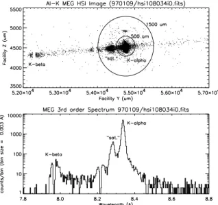
Detailed images and measurements of HETG-diffracted X-ray lines were made at XRCF to study the line response function, LRF (Marshall et al. 1997). For example, Figure 14 shows an image and resulting spectrum of the MEG 3rd
-order diffracted Al-K line complex recorded at XRCF with the non-flight High Speed Imager, HSI, micro-channel plate detector. Measurements of various parameters related to the LRF are
de-scribed in the following paragraphs and summa-rized in Table 1.
Grating Angles By measuring the centroid of the diffracted images from HEG and MEG grat-ings, the opening angle between HEG and MEG was measured to be very close to the 10 degree design value, see Table 1.
Grating Period and Rowland Spacing
Mea-surements using X-ray lines of known wavelength were used to confirm the values of the grating periods and measure the HETG Rowland spac-ing at XRCF. The ratio of HEG to MEG period determined from measurements agrees within a 100 ppm uncertainty with the ratio expected based on the lab-derived periods in Table 1. Adopting these periods and an Al-K energy of 1.4867 keV the HETG Rowland spacing as-operated at XRCF was determined and is given in Table 1.
LRF Core Measurements In order to see if
the insertion of the HETG modified the zeroth-order image, HSI exposures were taken in Al-K X-rays of each shell of the HRMA illuminated in turn with no grating present. With the HETG in-serted images were obtained for the zeroth-order of the MEG-only and HEG-only through each of four quadrants. The HRMA exposures for shells 1 and 3 (4 and 6) were then compared with the com-bined MEG (HEG) zeroth-order quadrant images. Comparing the projections of the two data sets binned to 10 µm shows good agreement in shape, within 10-20% in each bin, over 2 decades of the PSF intensity, covering the spatial range ±150µm. In particular, the inner core of the HRMA PSF at XRCF shows a FWHM of ≈ 42µm and insertion of the HETG adds no more than an additional FWHM of ≈ 20µm, i.e., at most increasing the FWHM from 42 to 46µm.
For diffracted images, precise measurements were made of the core of the PSF by using slit scans of the Mg-K 1.254 keV (9.887 ˚A) line in the bright orders m = 0, 1, 2 for HEG and m = 0, 1, 3 for MEG. Scans were made along both the disper-sion and cross-disperdisper-sion directions using 10 µm and 80 µm wide slits in front of proportional counter detectors. To create simulated XRCF slit scan data, a spectral model of the XRCF source
was folded through a MARX (Wise et al. 2000) ray-trace simulation tailored to XRCF parameters that affect the intrinsic LRF (most importantly: finite source distance, finite source size, and an additional 0.3 arc seconds of HRMA blur.) The intrinsic FWHM of the line spectral model and the period variation dp/p values for each grating type (HEG, MEG) were then adjusted in the simula-tion. Good agreement with the XRCF data is ob-tained when the core of the Mg-K line is modeled as a Gaussian with an E/dE = 1800, the HEG gratings have a dp/p value of 146 ppm rms and the MEG gratings have a dp/p of 235 ppm rms. These values are larger than expected from the individual LR results and likely represent slight additional distortions introduced during the facet-to-HESS alignment and bonding process; however, they are within our design goal of 250 ppm.
Mis-aligned MEG gratings As seen and
noted in Figure 14, a small “ghost image” is visible in the cross-dispersion direction “above” the diffracted Al-K line. Analyzing similar im-ages taken quadrant-by-quadrant as well as a very (65.5 mm!) defocused image of the MEG 3rd order which isolated the individual grating facet images (Marshall et al. 1997), we were able to demon-strate that this and other ghost images closer to the main image were created by individual MEG grating facets whose grating bars are “rolled” from the nominal orientation. In all, six of the 192 MEG facets have roll offsets in the range of 3 to 25 arc minutes - greatly in excess of the laboratory align-ment system measurealign-ment results. The individual facets were identified, for details see HETG (2002), and all came from fabrication Lot #7 — the only lot which was produced with prototype fabrica-tion tooling during the membrane mounting step (Fig. 8g). It was subsequently demonstrated in the laboratory (by Richard Elder) that inserting a stressed polyimide membrane between the photo-elastic modulator and the grating, see Figure 13, could create a shift in the alignment angle of order arc minutes and which varied with applied stress. Note in Figure 13 that the polyimide layer of the facet being aligned is in the optical path between the polarization modulated alignment laser and the grating bars. This clearly suggests that stress birefringence (Born & Wolf 1980, p. 703) in the grating’s polyimide membrane introduces
unin-tended bias offsets in the optical measurement of the grating bar angles, effectively causing their mis-alignment by these same bias angles.
Roll variations Mg-K slit scans, described
above, were also taken in the cross-dispersion di-rection and provide a check on the roll variations and alignment of the grating facets, the main con-tributor to cross-dispersion blur beyond the mirror PSF and Rowland astigmatism. Cross-dispersion distributions were input to the ray-trace simula-tions and adjusted to agree with the data. The resulting HEG and MEG roll distributions each have an rms variation of 1.8 arc minutes. The MEG distribution is close to Gaussian while the HEG shows a clear two-peaked distribution with the peaks separated by 3 arc minutes. These vari-ations are larger than the 0.42 arc minute rms value expected from the polarization alignment laboratory tests. The most likely cause is poly-imide membrane effects similar to those which produced the mis-aligned MEGs but occurring at a lower level. The mis-aligned gratings and the roll distributions are explicitly modeled in MARX simulations.
Wings on the LRF Wide-slit scans of the Mg-K line were used to set an upper limit to any “wings” on the LRF introduced by the HETG
gratings. The Mg-K PSF was scanned by an
80 µm x 500 µm slit for the MEG and HEG mir-ror shell sets separately. These scans were fit, us-ing ISIS (Houck & DeNicola 2000) software, by a Gaussian in the core and a Lorentzian in the wings, as shown in Figure 15. Quantitatively the wing level away from the Gaussian core can be expressed as:
LW(∆λ) = AGCwing/(∆λ)2 (7)
where LW is the measured wing level in counts/˚A,
AGis the area of the Gaussian core in counts, and
∆λ = λ − λ0 is the distance from the line
cen-ter. The strength of the wing is given by the value Cwing which has units of “fraction/˚A × ˚A2” or
(more opaquely) just “˚A”. Using this formalism the observed wing levels were determined for the HEG 1st and 2nd orders and the MEG 1st and
3rd orders, giving values of 8.6, 7.1, 12.2, and 7.8
due to the intrinsic Lorentzian shape of the Mg-K line itself (Agarwal 1991, p.108) with the reason-able value of a natural linewidth of 0.0035 ˚A. The remaining wing level can be largely explained as due to the wings of the HRMA PSF itself: be-cause the LRF is essentially the HRMA PSF dis-placed along the dispersion direction by the grat-ing diffraction, wgrat-ings of the mirror PSF directly translate into wings on the grating LRF. Subtract-ing these values we get an estimate of (upper limit on) the contribution to the wing level by the HEG and MEG gratings per se, as given in Table 1. Scatter beyond the LRF Tests were also car-ried out at XRCF to search for any response well outside of the discrete diffraction orders. A high-flux, monochromatic line was created by tuning the Double Crystal Monochromator (DCM) to the energy of a bright tungsten line from the rotat-ing anode X-ray source. The HEG gratrotat-ing set did show anomalous scattering of monochromatic ra-diation (Marshall et al. 1997), in particular a small flux of events with significant deviations from the integer grating orders are seen concentrated along the HEG dispersion direction, Figure 16. No such additional scattering is seen along the MEG dis-persion direction.
The origin of this scattering was understood using an approximate model of a grating with simple rectangular grating bar geometry that in-corporates spatially correlated deviations in the bar-parameters (Davis, Marshall, Schattenburg, & Dewey 1998), i.e., there is Fourier power in the grating structure at spatial periods other than the dominant grating period and its harmonics. Ex-pressions for the correlations and the scattering probability were derived and then fit to the exper-imental data. The resulting fits, while not perfect, do reflect many of the salient features of the data, confirming this as the mechanism for the scatter-ing. The grating-bar correlations deduced from this model lead to a simple physical picture of grating bar fluctuations where a small fraction of the bars (0.5%) have correlated deviations from their nominal geometry such as a slight leaning of the bars to one side. It is reasonable that the HEG gratings, with their taller, narrower bars, are more susceptible to such deviations than the MEG, which does not show any measurable scat-ter.
In practice the scattered photons in HEG spec-tra are excluded from analysis through order selec-tion using the intrinsic energy resoluselec-tion of ACIS: the energy of the scattered photon is significantly different from the energy expected at its apparent diffraction location. This is not true for scattered events that are close to the diffracted line image and they will make up a local low-level pedestal to the HEG LRF. However, the power scattered is small compared to the main LRF peak, generally contributing less than 0.01 % of the main response into a three FWHM wide region (0.036 ˚A) and less than 1 % in total.
ACIS Rowland Geometry An XRCF test was
designed to verify the Rowland geometry of the HETGS, in particular that all diffracted orders si-multaneously come to best focus in the dispersion-direction. Data were taken with each of four quad-rants of the HRMA illuminated, allowing us to de-termine the amount of defocus for each of the mul-tiple orders imaged by the detector. Because of the astigmatic nature of the diffracted images, the ax-ial location of “best focus” depends on which axis is being focused. The results of this test (Stage & Dewey 1998) were limited by the number of events collected in the higher-orders; however it was concluded that i) the astigmatic focal prop-erty was confirmed, ii) the HEG and MEG focuses at XRCF differed by 0.32 mm as expected from HRMA modeling, and iii) the ACIS detector was tilted by less than 10 arc minutes about the Z-axis.
4.2. Efficiency and Effective Area
Mea-surements
A major objective of XRCF testing was to mea-sure the efficiency of the fully assembled HEG and MEG grating sets and the effective area of the full HRMA + HETG + ACIS system. The HETGS effective area or ARF (Davis 2001a) for a given grating set or part, indicating HEG or MEG, and diffraction order m may be expressed in simplified form as:
AP,m(λ) = MP(λ) gP,m(λ) Q(λ, ~σ) (8)
where λ denotes the dependence on photon wave-length (or energy) and the three contributing terms are the HRMA effective area MP(λ) for
the relevant part (e.g., MEG combines the area of HRMA shells 1 and 3), the effective HETG grating efficiency for the part-order gP,m(λ), and
the ACIS-S quantum detection efficiency Q(λ, ~σ). The ~σ parameter signifies a dependence on the focal-plane spatial location, e.g., at “gap” loca-tions between the individual CCD detector chips we have Q(λ, ~σgap) = 0. Although not explicitly
shown, this ACIS efficiency also depends on other parameters, in particular CCD operating temper-ature and event grade selection criteria.
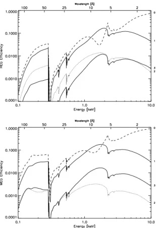
The grating effective efficiency gP,m(λ) is
de-fined as: gP=MEG[HEG],m(λ) = P s=1,3[4,6]Ms(λ)gs,m(λ) P s=1,3[4,6]Ms(λ) (9) where s designates the HRMA shell (the number-ing system is a legacy from the original AXAF HRMA design which had 6 shells; shells 2 and 5 were deleted to save weight and cost). The grat-ing efficiency values gs,m(λ) are the average of the
facet efficiency models derived from X-GEF data for all facets on shell s multiplied by a shell vi-gnetting factor (primarily the fraction of the beam not blocked by grating frames), Table 1. The val-ues of these (single-sided) effective efficiencies are plotted for zeroth through third order in Figure 17 for the HEG and MEG grating sets; they are ver-sion “N0004” based on the laboratory measured facet efficiencies and using our updated optical constants.
Diffraction Efficiency Measurements In
principle the diffraction efficiency of the HETG can be measured as the ratio of the flux of a monochromatic beam diffracted into an order di-vided by the flux seen when the HETG is removed from the X-ray beam, a “in over grating-out” measurement. If the same detectors are used in the measurements then their properties cancel and the efficiency can be measured with few sys-tematic effects. In early testing at XRCF the HEG and MEG diffraction efficiencies were measured using non-imaging detectors, a flow proportional counter and a solid state detector (Dewey et al. 1997; Dewey, Drake, Edgar, Michaud, & Ratzlaff 1998). The detector’s entrance aperture could be defined by a pinhole of selectable size, typically
0.5 to 10 mm in diameter.
The main complication of these non-imaging measurements results from the complexity of the source spectra and the limited energy resolution of the detectors compared to that of the HETGS. The Electron Impact Point Source (EIPS) was used to generate K and L lines of various elements, in particular C, O, Fe, Ni, Cu, Mg, Al, Si, Mo, Ag, and Ti. As Figure 14 shows, the “line” typ-ically consists of several closely spaced lines. For the “grating-in” dispersed measurement only some fraction of these “lines” fall in the pinhole aper-ture and are detected e.g., consider the the 500 µm aperture indicated in the figure. In contrast, the “grating out” measurement includes all of the lines and any local continuum within the energy reso-lution element of the low-resoreso-lution detector. In order to make a correction for this effect, spectra at HETG resolution, similar to Figure 14, were collected for each X-ray line of interest and used to calculate appropriate correction factors, rang-ing from a few percent to a factor of two.
The resulting XRCF efficiency measurements for the HEG and MEG first orders are shown in Figure 18 along with the laboratory-based values (solid lines, from Figure 17.) The error bars here, in addition to counting statistics, include an es-timate of the systematic uncertainty introduced in the correction process described. These results confirm the efficiency models derived from X-GEF measurements at the 10-20 % level but also sug-gest possible systematic deviations. Because these deviations are small we waited for flight data be-fore considering any corrections to the efficiency values.
Absolute Effective Area Absolute effective
area measurements were performed at the XRCF with the flight ACIS detector, in particular the ACIS-S consisting of a linear array of 6 CCD de-tector chips designated S0 through S5 (or CCD ID = 4–9). Devices at locations S1 and S3 are back illuminated (BI) CCDs with improved low-energy response. S3 is at the focal point, so it detects zeroth order and is often used without the HETG inserted for imaging observations; S1 is placed to detect the cosmically important lines of ionized oxygen with enhanced efficiency. Note that there are small gaps between the ACIS-S CCDs with sizes determined by the actual chip focal plane
lo-cations.
The 1st-order HETGS effective area can be di-vided into 5 regions where different physical mech-anisms govern the effective area of the system (var-iously shown in Figures 3, 17, 20, and 21):
below 1 keV – Absorption by the polyimide membranes of the gratings and the ACIS op-tical blocking filter and SiO layers limit the effective area and introduce structure, with absorption edges due to C, N, O, and Cr. 1-1.8 keV– The phase effects of the partially transparent gratings enhance the diffraction efficiency.
1.8-2.5 keV– Edge structures are due to the Si (ACIS), the Ir (HRMA), and Au (grat-ing).
2.5-5.5 keV – Effective area is slowly vary-ing, with some low-amplitude Ir (HRMA) and Au (HETG) edge structure. The effi-ciency is also phase-enhanced in this region especially for the HEG.
5.5-10 keV– The mirror reflectivity, grating efficiency, and ACIS efficiency all decrease with increasing energy leading to a progres-sively steepening decline.
The energy range from 0.48 to 8.7 keV was sam-pled at over 75 energies using X-rays produced by three of the sources of the X-Ray Source System (Kolodziejczak et al. 1995). The Double Crystal Monochromator (DCM) provided dense coverage of the range 0.9 to 8.7 keV; the High Resolution Erect Field (grating) Spectrometer (HiREFS) pro-vided data points in the 0.48 to 0.8 keV range; and X-ray lines from several targets of the Electron Im-pact Point Source (EIPS) covered the range from 0.525 keV (O-K) to 1.74 keV (Si-K).
The absolute effective area was measured as the ratio of the focal plane rate detected in a line to the line flux at the HRMA entrance aperture. A set of four Beam Normalization Detectors (BND) were located around the HRMA and served as the prime source of incident flux determination. The ACIS detector was defocused by 5 to 40 mm to reduce pileup caused when more than one photon arrives in a small region of the detector during a single integration (Davis 2001b, 2003) by spreading the
detected events over a larger detector area as seen in Figure 19. A variety of analysis techniques and considerations were applied to analyze these data (Schulz, Dewey, & Marshall 1998), chief among them for the monochromator data sets were beam uniformity corrections to the effective flux based on extensive measurements and modeling carried out by the MSFC project science group (Swartz et al. 1998). Other corrections were made for line deblending and ACIS pileup. Uncertainties in the measurements were assigned based on count-ing statistics and estimated systematics; typically each measurement has an assigned uncertainty of order 10 %.
Representative results are shown for the MEG m = −1 in Figure 20, using ACIS chips S0, S1, S2, and S3, and for the HEG m = +1 in Figure 21, detected on chips S3, S4, and S5. Measurements of the HETG combined zeroth order are shown in Figure 22. The data indicate that we are close to realizing our goal of a 10 % absolute effective area calibration for the first order effective area. The measurement-model residuals are seldom outside a ±20 % range for both the HEG and MEG first-order areas. Systematic variation of the residuals appear at a level of order −20 % in the energy range below 1.3 keV; there is agreement better than 10 % in the 2.5 to 5 keV range, The regions of greater systematic variation, 1.3 to 2.5 keV and above 5 keV, are most likely dominated by uncom-pensated DCM beam uniformity effects and ACIS pileup effects, respectively.
Effective area measurements for |m| ≥ 2 were also carried out with the flight focal plane detec-tors (Flanagan, Schulz, Murray, Hartner, & Pre-dehl 1998) and show agreement at the 20 % level for HEG second and MEG third orders.
Relative Effective Area In order to probe
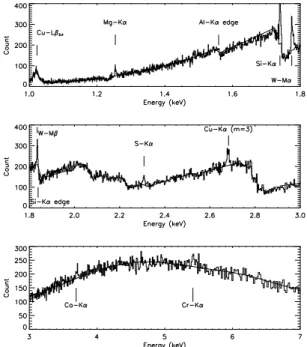
for small scale spectral features in the HETGS response we performed tests at XRCF using a very bright continuum source (Marshall, Dewey, Schulz, & Flanagan 1998). The Electron Impact Point Source (EIPS) was used with Cu and C an-odes and operated at high voltage and low current in order to provide a bright continuum over a wide range of energies. The ACIS-S was operated in a rapid read-out mode (“1x3” continuous clocking mode) to discriminate orders and to provide high throughput.
High-count spectra were created from the data and compared to a smooth continuum model passed through the predicted HETGS effective area, Figure 23. Many spectral features are ob-served, including emission lines attributable to the source spectrum. We find that models for the HETGS effective area predict very well the structures seen in the counts spectrum as well as the observed fine structure near the Au and Ir M edges where the response is most complex. Edges introduced by the ACIS quantum efficiency (QE) and the transmission of its optical blocking filter are also visible, the Si K and Al K edges respec-tively. By comparing the positive and negative dispersion regions, we find no significant efficiency asymmetry attributable to the gratings and we can further infer that the QEs of all the ACIS-S frontside illuminated (FI) chips are consistent to ±10 %.
5. Five Years of Flight Operation
5.1. Flight Data Examples
The first flight data from the HETG were ob-tained on August 28, 1999 while pointing at the active coronal binary star Capella. Subsequent observations of this and other bright sources pro-vided in-flight verification and calibration. The instrument performance in orbit is very close to that measured and modeled on the ground. A re-cent summary of Chandra’s initial years is given by Weisskopf et al. (2004) and Paerels & Kahn (2003) review some aspects of high resolution spectroscopy performed with Chandra and XMM-Newton.
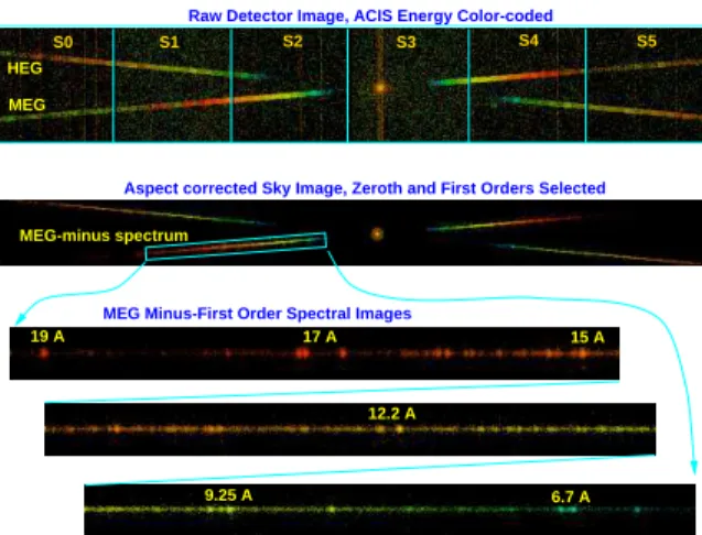
Figure 24 shows 26 ks of data from Capella. The top panel shows an image of detected events on the ACIS-S detector with the image color indi-cating the ACIS-determined X-ray energy. In this detector coordinate image, the features are broad due to the nominal dither motion in which the spacecraft pointing is intentionally “dithered” to average over small-scale detector non-uniformities. The ACIS-S chips are numbered S0 to S5 from left to right, with the aim point in S3 where the bright undispersed image is visible and includes a vertical frame-transfer streak. HETG-diffracted photons are visible forming a shallow “X” pattern. The middle panel shows an image after the data have been aspect corrected and data selections applied
to include only valid zeroth and first order events. The lower set of panels shows an expanded view of the MEG, m = −1 spectrum with emission lines clearly visible. The observed lines and instrument throughput are roughly as expected (Canizares et al. 2000).
As a demonstration of the high resolving power of the HEG grating, a closeup of the 9.12 ˚A to 9.35 ˚A spectral region of a Capella observation is shown in Figure 25. The three main lines seen here are from n = 2 to n = 1 transitions of the He-like Mg+10ion, designated “Mg XI”; a resolving power
of ≈ 850 is being achieved here with a FWHM of ≈ 1.6 eV.
5.2. Flight Instrument Issues
Since the HETGS is a composite system of the HRMA, HETG, ACIS, and spacecraft systems, the HETGS flight performance is sensitive to the prop-erties of all of these systems. The various flight issues that have arisen in the past 5 years are summarized here by component and their effect on the HETGS performance is mentioned. A com-plete account of these issues is beyond the scope of this paper; further details of the in-flight HETG calibration are presented in Marshall, Dewey, & Ishibashi (2004). See also documents and refer-ences from the Chandra X-ray Center (CXC 2004) which also archives and maintains specific calibra-tion values and files in the Chandra Calibracalibra-tion Database, CALDB, along with extensive release notes.
5.2.1. HRMA issues
The HRMA (van Speybroeck et al. 1997) is the heart of the observatory and has maintained a crisp, stable focus for five years; the commanded focus setting has remained the same for five years. The HETG resolving power has remained stable as well indicating stability of the grating facets and overall assembly. Details of the HRMA PSF in the wings are still being worked but this has min-imal effect on the HETG LRF/RMF in practical application.
The only issue arising in flight related to the HRMA is seen as a slight step-increase (15 %) in effective area in the region near the Ir Medge -seen clearly in HETGS spectra. A model based on the reflection effect of a thin contamination layer
on the HRMA optical surfaces agrees reasonably with the deviations seen, Figure 26, implying a hy-drocarbon layer thickness of 20±5 ˚A. At present there is no evidence that the layer thickness is changing significantly with time; detailed model-ing and updates to the calibration products are in progress.
5.2.2. ACIS issues
In the first flight data sets slight wavelength differences were seen between the plus and minus orders indicating a few pixel error in our knowl-edge of the relative locations of the ACIS-S CCDs. The ACIS geometry values were adjusted for this in 1999 to an accuracy of ∼ 0.5 pixels. As a by-product of our HETG LSF work, see below, these values have been updated a second time to an ac-curacy of ∼ 0.2 pixels and they show a stability at this level over the first five years of flight.
The ACIS pixel size as-fabricated was precisely quoted as 24.000 µm and this value was used for initial flight data analysis. However it was later realized that this value was for room tempera-ture - at the flight operating temperatempera-tures of or-der −120 C the pixel size was determined to be 23.987 µm and this value has been incorporated into the analysis software, etc.
Order separation is performed using the intrin-sic energy resolution of the ACIS CCDs, as demon-strated in Figure 27 for a Capella observation. ACIS suffered some radiation damage early in the mission which degraded the energy resolution of the front-illuminated, FI, chips (Townsley et al. 2000); relevant to the HETGS are FI chips: S0, S2, S4, and S5. However, as seen in the figure, the resolution of those CCDs is still sufficient to permit clean separation of the HETG orders. The CXC pipeline software generally includes 95 % of the first-order events in its order selection; the ex-act frex-action depending on CCD and energy is cal-culated and included in the creation of HETGS ARF response files.
The ACIS detector suffers from pileup (Davis 2001b) and this was expected in the bright zeroth-order image. However, pileup also shows up in the dispersed spectra of bright sources and/or bright lines; algorithms have been developed to amelio-rate this pileup (Davis 2003).
Early in the mission there were indications in
LETG-ACIS data that the C-K edge of the ACIS optical blocking filter, OBF, was deeper than pre-dicted. Later it was realized that a contaminant was building up on the ACIS OBF and hence the effective ACIS QE was decreasing (Marshall et al. 2004). The main spectral, temporal, and spatial effects of this contaminant have now been incor-porated into Chandra responses; the composition and properties of the contaminant are the focus of continued measurement and modeling.
Comparison of the plus and minus orders of the HETGS lead to a measurement of a discrepancy of the QEs of the ACIS FI CCDs compared to ACIS back illuminated CCDs (S1, S3.) This issue is recently resolved into two components: the FI devices suffer from cosmic-ray dead time effects of order 4 % and the BI QEs are actually somewhat larger than initially calibrated. The BI QEs were updated in August 2004 (CALDB 2.28) and are thus now included in HETGS ARFs.
5.2.3. HETG issues
All the essential parameters for the HETG in flight are the same or consistent with the ground values. Some notable quantities are discussed be-low.
Clocking Angle: The flight angles of the HEG and MEG dispersion axes measured on the ACIS-S are given in Table 1; these values are in agreement with the XRCF-measured values.
Rowland Geometry and Spacing: An accurate ac-count of the Rowland geometry and spacing is crucial to achieve the best focus of the dispersed spectra on the detector. The Rowland geome-try of the HETG was demonstrated during ini-tial plate-focus tests: dispersed line images from a range of wavelengths came to their best dispersion-direction focus at a common detector focus value, which agreed with the ACIS-S3 best-imaging focus value within 50 µm. The spacing of the HETG from the focal plane, the Rowland spacing, ap-peared initially to be off from the expected value until the ACIS pixel size change with tempera-ture was included (previous section). Currently the HETG Rowland spacing in flight, given in Ta-ble 1, is the value produced by ground installation metrology.
Grating Period: The accuracy of the HETG-measured wavelength depends strongly on the
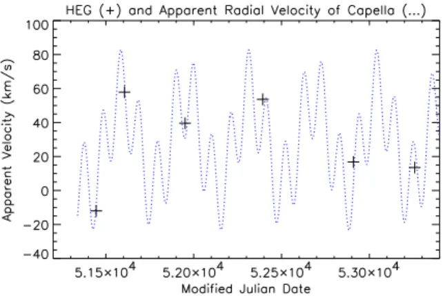
as-signed grating period. For the first years of use, the grating periods of the HEG and MEG were set to the laboratory measurement results. However, recent analysis of Capella data over 5 years shows the MEG-derived line centroid to be off by 40.2 ±5 km s−1 compared to the, apparently accurate,
HEG values, see Figure 28. Hence the MEG pe-riod has recently (CALDB version 3.0.1, Febru-ary 2005) been set to 4001.95 ˚A, which makes the MEG/HEG line centroids mutually consistent. Note that the stability of the wavelength scale is good to 10 km s−1 or 30 ppm over 5 years.
Dispersion and Cross-Dispersion Profiles: Re-cently the HETG line response functions (LRFs) have been modeled as a linear combination of two Gaussians and two Lorentzians to encode im-proved fidelity with the latest results of MARX ray-trace models (Marshall, Dewey, & Ishibashi 2004); these LRF products are available in Chan-dra CALDB versions 2.27 and higher. A Capella in-flight calibration data set (ObsID 1103) has been used to verify the quality of the LRFs. Us-ing a multi-temperature APED thermal model (Brickhouse 1996), the He-like line complex of Mg XI has been fitted with the grating line re-sponse functions. Thermal broadening of Mg XI species has been taken into account in order to measure its line width properly. Figure 25 shows the result of this model fitting. The derived line widths are essentially in agreement with having no excess broadening, as expected for static coro-nal emission. Note that the wings of the grating line response functions, two orders of magnitude below the peak when a few FWHMs away, are generally well below the actual continuum and pseudo-continuum levels in celestial sources, and so flight dispersed data does not help calibrate the wings of LRF in general.
In the cross-dispersion direction, we parame-terize the fraction of energy “encircled” in an ar-bitrary rectangular region (the encircled energy fraction, or EEF) and include this in the analy-sis software. The calibration values encoded into LRFs are generally consistent with observations. An uncertainty of 1 – 3% may be introduced by the EEF term, though other quantitative uncer-tainties (e.g., HRMA effective area) are compara-ble or greater at this point in HETGS calibration. HETG Efficiency Calibration: After five years of flight operation the efficiencies of Figure 17, based
on the facet laboratory measurements, have not been adjusted and are still used to create ARFs for flight observations. Likewise no additional fea-tures or edges have been ascribed to the HETG instrument response beyond what is in these cali-bration files. Comparing HEG and MEG spectra of bright continuum sources, there is data to sup-port making a relative correction of the HEG and MEG efficiencies to bring their measured fluxes into agreement. This relative efficiency correction is small, in the range 0 % to -7 % if applied to the MEG, and varies smoothly in the 2 ˚A to 15 ˚A range. This final “dotting the i” of HETG calibra-tion is nearing complecalibra-tion and will be included in upcoming CXC calibration files.
5.3. Discussion
As the minimal effect on the HETGS perfor-mance of the various flight issues described above indicates, the HETGS has and is performing essen-tially as designed yielding high-resolution spectra of a broad range of astrophysical sources. Some calibration issues are still being addressed, but these are at the ∼ 10 % level in the ARF and the fractions-of-a-pixel level in the grating LRF/RMF. It is useful to put the Chandra gratings’ perfor-mance in perspective with each other and with the Reflection Grating Spectrometer, RGS, on XMM-Newton. The effective areas for these grat-ing instruments are shown in Figure 29; note the complementary nature of the instruments in vari-ous wavelength ranges. The advance in resolving power these dispersive instruments have provided is clearly seen in Figure 30 in comparison to the ACIS CCD resolving power values shown there as well. A line for the resolving power of a 6 eV FWHM micro-calorimeter (e.g., Astro-E2) is plot-ted as well showing the uniqueness of the grating instruments in the range below 2 keV.
The high resolution and broad bandpass of the HETGS have made it the instrument of choice for many observers. In the first five years of Chandra operation, the HETGS was used in over four hun-dred observations totaling approximately 20 Ms of exposure time. This represents about 17 % of Chandra’s total observation time for that pe-riod. As is typical of spectroscopy at other wave-lengths, HETGS observations tend to be long, ranging from tens of ks for bright Galactic sources to hundreds of ks for active galactic nuclei (AGN).
A review of the results of these observations is out-side the scope of this paper; some examples can be found in Weisskopf et al. (2002, 2004) and Paerels & Kahn (2003).
Acknowledgments The HETG is the product
of nearly two decades of research and development in the MIT Center for Space Research, now the MIT Kavli Institute (MKI), to adapt the tech-niques of micro- and nano-structures fabrication developed primarily for micro-electronics to the needs of X-ray astronomy. The initial concept emerged from nanostructures research conducted by one of us (H.I.S. and collaborators) in the MIT Nano Structures Laboratory of the Research Lab-oratory of Electronics (and previously at MIT Lin-coln Laboratory). We thank Al Levine, Pete Tap-pan, and Bill Mayer for initial HETG design eval-uations.
The Space Nanotechnology Laboratory was es-tablished in CSR under the leadership of HETG Fabrication Scientist M.L.S. to advance the tech-nology and then execute the fabrication of the flight hardware. Significant processing support was provided by the MIT Microsystems Technol-ogy Laboratory. Fabrication engineering support was provided by Rich Aucoin, Bob Fleming, Pat Hindle, and Dave Breslau. Facet fabrication was carried out by Jeanne Porter, Bob Sission, Roger Millen, and Jane Prentiss.
D.D., Instrument Scientist, M.M., Systems En-gineer, and K.A.F. led the overall design and ground calibration activities. J.E.D. provided ef-ficiency modeling algorithms and software. De-sign and test engineering support was provided by Chris Pak, Len Bordzol, Richard Elder, Don Humphries, and Ed Warren. Facet testing was carried out by Mike Enright and Bob Laliberte who assembled the flight HETG.
H.L.M. carried out much of the XRCF test planning and analyses. M.W. and D.P.H. pro-vided modeling and analysis support. N.S.S. an-alyzed key XRCF data as did Sara Ann Taylor and Michael Stage. Many of the authors were in-volved in flight calibration; K.I. carried out de-tailed flight LSF work. Finally, focus and progress were maintained under the overall leadership of C.R.C., Instrument Principal Investigator, sup-ported by T.L.M. as Project Scientist through
much of the design and development phase and E.B.G. as Project Manager (Galton 2003).
The HETG team acknowledges conspicuous and inconspicuous support from our colleagues at the CSR and from the many groups involved in the Chandra project, specifically MSFC Project Science, Smithsonian Astrophysical Observatory, TRW, and Eastman Kodak. We thank John Kra-mar and colleagues at NIST for LR period cali-bration.
Finally, we thank our fellow citizens: this work was supported by the National Aeronau-tics and Space Administration under contracts NAS8-38249 and NAS8-01129 through the Mar-shall Space Flight Center.