Approaches to multi-agent learning
by
Yu-Han Chang
Submitted to the Department of Electrical Engineering and Computer
Science
in partial fulfillment of the requirements for the degree o
Doctor of Philosophy
at the
MASSACHUSETTS INSTITUTE OF TECHNOLOGY'
"May 2005
@
Massachusetts Institute of Technology 2005. All rights reserved.
A uthor ...
Department of Electrical Engineerin4(and Computer Scieni3
May 20, 2005
Certified by ...
(
L l . . . .
Leslie Pack Kaelbling
Professor of Computer Science and Engineering
Thesis Supervisor
RKER
Accepted by
Arthur C. Smith
Chairman, Department Committee on Graduate Students
MASSACHUSETTS IN E OF TECHNOLOGY OCT
2005
MASSACHUSETTS INSTJE OF TECHNOLOGYOCT 2
12005
LIBRARIES
...
. .
Approaches to multi-agent learning
by
Yu-Han Chang
Submitted to the Department of Electrical Engineering and Computer Science on May 20, 2005, in partial fulfillment of the
requirements for the degree of Doctor of Philosophy
Abstract
Systems involving multiple autonomous entities are becoming more and more promi-nent. Sensor networks, teams of robotic vehicles, and software agents are just a few examples. In order to design these systems, we need methods that allow our agents to autonomously learn and adapt to the changing environments they find themselves in. This thesis explores ideas from game theory, online prediction, and reinforcement learning, tying them together to work on problems in multi-agent learning.
We begin with the most basic framework for studying multi-agent learning: re-peated matrix games. We quickly realize that there is no such thing as an opponent-independent, globally optimal learning algorithm. Some form of opponent assump-tions must be necessary when designing multi-agent learning algorithms. We first show that we can exploit opponents that satisfy certain assumptions, and in a later chapter, we show how we can avoid being exploited ourselves.
From this beginning, we branch out to study more complex sequential decision making problems in multi-agent systems, or stochastic games. We study environments in which there are large numbers of agents, and where environmental state may only be partially observable. In fully cooperative situations, where all the agents receive a single global reward signal for training, we devise a filtering method that allows each individual agent to learn using a personal training signal recovered from this global reward. For non-cooperative situations, we introduce the concept of hedged learning, a combination of regret-minimizing algorithms with learning techniques, which allows a more flexible and robust approach for behaving in competitive situations. We show various performance bounds that can be guaranteed with our hedged learning algorithm, thus preventing our agent from being exploited by its adversary. Finally, we apply some of these methods to problems involving routing and node movement in a mobilized ad-hoc networking domain.
Thesis Supervisor: Leslie Pack Kaelbling
Acknowledgments
I am indebted to my advisor Leslie Kaelbling for her vast stores of wisdom, her generous capability for finding time to share it, her invaluable guidance and encour-agement, and her infinite patience while I searched for my research bearings. I would also like to thank my thesis committee members, Tommi Jaakola, Michael Littman, and John Tsitsiklis, for their helpful advice and insights. This thesis would not have been possible without the enduring support of my parents, who have encouraged me in the pursuit of knowledge and wisdom throughout my life, and Tracey Ho, who has been my love, light, and inspiration throughout the writing of this thesis.
Contents
1 Introduction
1.1 M otivation . . . . 1.2 The approach . . . . 1.3 Scaling up ... ...
1.4 Highly complex domains . . . . 1.5 A specialization: cooperative, single-designer systems
1.5.1 Mobilized ad-hoc networking . . . . 1.6 Thesis contributions . . . . 2 Background
2.1 Repeated games
2.1.1 Mathematical setup . . . . 2.1.2 Prior work . . . . 2.1.3 Solving for Nash equilibria . . . . 2.1.4 Correlated Nash equilibria . . . . 2.1.5 Game theoretic perspective of repeated games 2.2 Regret-minimization and online learning . . . .
2.2.1 Prior work . . . . 2.2.2 A reactive opponent . . . . 2.3 F iltering . . . . 2.4 POMDP methods . . . . 2.4.1 Markov decision processes . . . . 2.5 Mobile ad-hoc networking . . . .
21 22 24 24 25 27 27 30 33 . . . . 3 3 . . . . 34 . . . . 37 . . . . 39 . . . . 41 . . . . 41 . . . . 44 . . . . 44 . . . . 45 . . . . 47 . . . . 48 . . . . 50 . . . . 52
2.5.1 Node movement . . . . 52
2.5.2 Packet routing . . . . 52
2.5.3 Learning . . . . 53
3 Learning in repeated games 55 3.1 A new classification . . . . 56
3.1.1 The key role of beliefs . . . . 59
3.1.2 Existing algorithms . . . . 59
3.1.3 The policy hill climber . . . . 62
3.2 A new class of players and a new algorithm . . . . 63
3.2.1 A new algorithm: PHC-Exploiter . . . . 64
3.2.2 Analysis . . . . 66
3.2.3 Experimental results . . . . 68
3.3 Combinations of methods . . . . 69
3.4 Conclusion . . . . 71
4 Large sequential games 75 4.1 The problem setting . . . . 75
4.1.1 Stochastic games . . . . 75
4.1.2 Partial observability . . . . 76
4.1.3 A motivating application . . . . 77
4.1.4 Credit assignment . . . . 78
4.2 A simple solution: Filtering the reward signal . . . . 79
4.3 Mathematical model . . . . 80 4.3.1 Kalman filters . . . . 81 4.3.2 Q-learning . . . . 82 4.3.3 Model solving . . . . 82 4.4 Algorithm . . . . 84 4.5 Experiments . . . . 85
4.5.1 Idealized noisy grid world . . . . 88
4.5.3 Mobilized ad-hoc networking . . . . 4.6 Discussion . . . . 4.6.1 Limitations . . . . 4.6.2 Model assumptions . . . . 4.6.3 Averaging rewards . . . . 5 Learning with uncertain models
5.1 Regret-minimizing methods . . . . 5.2 Mathematical setup . . . . 5.2.1 Reactive opponents . . . . 5.3 Extending the experts framework . . . . .
5.3.1 Evaluating all possible strategies 5.4 Learning Algorithms as Experts . . . .
5.4.1 Exam ple . . . . 5.5 The Hedged Learner . . . . 5.5.1 Naive approach . . . . 5.5.2 Hierarchical hedging . . . . 5.5.3 Practical comparisons . . . . 5.6 Experimental Results . . . . 5.6.1 Hedging between models . . . . 5.6.2 Non-stationary environments . . . . 5.7 Approximately optimal solutions to MDPs 5.8 Extensions . . . . 6 Mobilized ad-hoc networking
6.1 Domain overview . . . . 6.1.1 Performance benefits of mobility . . 6.2 The routing problem . . . . 6.3 The movement problem . . . . 6.4 Application of our methods . . . . 6.4.1 Routing . . . . 94 . . . . 96 . . . . 97 . . . . 99 . . . . 103 109 . . . . 110 . . . . 112 . . . . 112 . . . . 114 . . . . 117 . . . . 117 . . . . 119 . . . . 120 . . . . 121 . . . . 123 . . . . 126 . . . . 127 . . . . 127 . . . . 130 . . . . 131 . . . . 133 135 . . . . 135 . . . . 136 . . . . 138 . . . . 140 . . . . 142 . . . . 142
6.4.2 Movement ... 142 6.4.3 Basic Q-learning . . . . 143 6.4.4 Filtered learning . . . . 143 6.4.5 Gradient methods . . . . 144 6.4.6 Hedged learning . . . . 144 6.5 Empirical results . . . . 145
6.5.1 Empirical results for routing . . . . 145
6.5.2 Empirical results for movement . . . . 151
7 Conclusions and future work 157 7.1 Richer regret . . . . 160
7.2 The swarm . . . . 160
List of Figures
2-1 Some common examples of single-shot matrix games. . . . . 36 2-2 This figure shows an example of a network game. There are seven
players in this game, and the links between the players represent re-lationships between players that results in direct payoff consequences. For example, Player l's payoffs are only affected by its own actions, and the actions of Player 2 and Player 3. They are only indirectly affected by the action choices of the remaining four players, if Players 2 or Player 3's action choice is influenced by the rest of the players. . 39 2-3 This figure shows the Matching Pennies game in extensive form. Clearly,
the extensive form is a more general representation, since we can now allow the players to move sequentially and possess different information sets. Though not needed in this particular game, the extensive form representation can also include probabilistic choice nodes for "Nature", which can be used to account for randomness in the reward structure. 40
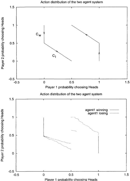
3-1 Theoretical (top), Empirical (bottom). The cyclic play is evident in our empirical results, where we play a PHC-Exploiter player 1 against a PHC player 2 in the Matching Pennies game. . . . . 72 3-2 Total rewards for the PHC-Exploiter increase as we gain reward through
each cycle, playing against a PHC opponent in the Matching Pennies gam e. . . . . 73
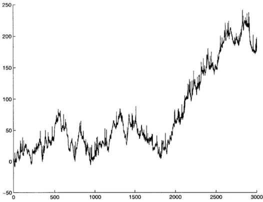
4-1 As the agent in the idealized single-agent grid world is attempting to learn, the reward signal value (y-axis) changes dramatically over time (x-axis) due to the noise term. While the true range of rewards in this grid world domain only falls between 0 and 20, the noisy reward signal ranges from -10 to 250, as shown in the graph at left. . . . . 85 4-2 Given the noisy signal shown in Figure 4-1, the filtering agent is still
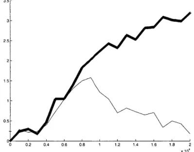
able to learn the true underlying rewards, converging to the correct relative values over time, as shown in the middle graph. . . . . 86 4-3 The filtering learning agent (bold line) accrues higher rewards over time
than the ordinary Q-learner (thin line), since it is able to converge to an optimal policy whereas the non-filtering Q-learner remains confused. 86 4-4 The filtering model-based learning agent (bold line) is able to learn an
optimal policy much quicker than the filtering Q-learning agent (thin line), since it is able to use value iteration to solve for the optimal policy once the personal reward signals have been accurately estimated. 87 4-5 This shows the dynamics of our 5x5 grid world domain. The states
correspond to the grid locations, numbered 1,2,3,4,...,24,25. Actions move the agent NS,E, or W, except in states 6 and 16, where any action takes the agent to state 10 and 18, respectively, shown by the curved arrows in the figure at left. . . . . 90 4-6 The optimal policy for the grid world domain is shown at left, where
multiple arrows at one state denotes indifference between the possibil-ities. A policy learned by our filtering agent is shown at right. The learning algorithm does not explicitly represent indifference, and thus always picks one action to be the optimal one. . . . . 90 4-7 Filtering agents are able to distinguish their personal rewards from
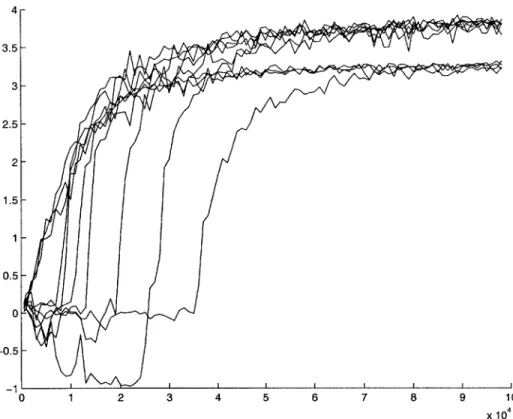
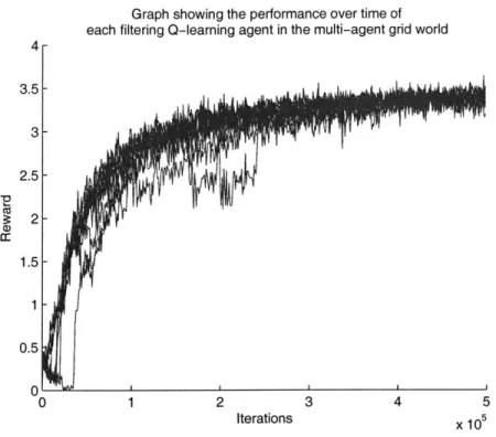
the global reward noise, and thus able to learn optimal policies and maximize their average reward over time in a ten-agent grid-world dom ain . . . . 91
4-8 Another graph showing that filtering Q-learners converge. Unlike Fig-ure 4-7, the exploration rate decay is slowed down, thus allowing all the agents to converge to the optimal policy, rather than being stuck
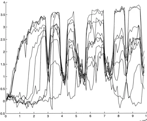
in the sub-optimal policy. . . . . 92 4-9 In contrast to Figure 4-7, ordinary Q-learning agents do not process
the global reward signal and can become confused as the environment changes around them. Graphs show average rewards (y-axis) within 1000-period windows for each of the 10 agents in a typical run of 10000 tim e periods (x-axis). . . . . 93 4-10 Once again, the filtered model-based agent is able to learn an optimal
policy in fewer simulation iterations than the filtered model-free
Q-learning agent. Note that the scale of the x-axis in this figure is different from the previous figures. . . . . 94 4-11 A snapshot of the 4x4 adhoc-networking domain. S denotes the sources,
R is the receiver, and the dots are the learning agents, which act as relay nodes. Lines denote current connections. Note that nodes may overlap . . . . . 95 4-12 Graph shows average rewards (y-axis) in 1000-period windows as
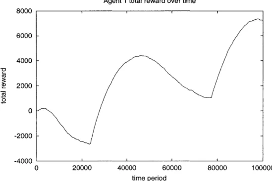
fil-tering Q-learner (bold line) and unfiltered Q-learner (thin line) agents try to learn good policies for acting as network nodes in the ad-hoc networking domain. The filtering agent is able to learn a better policy, resulting in higher network performance (global reward). Graph shows the average for each type of agent over 10 trial runs of 100000 time periods (x-axis) each. . . . . 96 4-13 Graph shows average rewards (y-axis) in 1000-period windows as
filter-ing model-based learners (bold line), filtered Q-learners (dashed line), and unfiltered model-based learners (thin line) try to learn good poli-cies for acting as network nodes in the ad-hoc networking domain. The trials are run on a 5x5 grid, with 4 sources, 1 receiver, and 13 learning nodes. ... ... 97
4-14 Graph shows average network connectivity in 1000-period windows as filtered Q-learning agents (dashed line), hand-coded agents (bold line), and random agents (dotted line) act as network nodes in the ad-hoc networking domain. The trials are run on a 5x5 grid, with 4 sources, 1 receiver, and 13 learning nodes. . . . . 98 4-15 This graph shows the distribution of the noise term over time in the
idealized noisy grid world simulation. The graph closely mimics that of a standard normal distribution, since the noise is drawn from a normal distribution. . . . . 100 4-16 This graph shows the distribution of the noise term over time in the
multi-agent grid world simulation. As we can see, the distribution still resembles a standard normal distribution even though the noise is no longer drawn from such a distribution but is instead generated by the other agents acting in the domain. . . . . 101 4-17 This graph shows the distribution of the estimated noise term over time
in the multi-agent ad-hoc networking simulation. This distribution only vaguely resembles a normal distribution, but is still symmetric about its mean and thus has low skew. . . . . 102 4-18 This graph shows the performance of a model-based learned using a
filtered reward signal (bold line) vs using an averaged reward signal (thin line). The averaging method does not work at all within the 25,000 time periods shown here. . . . . 104 4-19 Average rewards fluctuate over time, rendering the average reward an
inappropriate training signal since it does not give the agents a good
measure of their credit as a portion of the global reward signal. . . . 105
4-20 This graph shows the noise term evolving over time. While the additive term in each time period has a mean of zero, clearly the noise term bt increased as the agents learn good policies for behavior. . . . . 106
4-21 This graph shows the average additive noise over time. While the mean is very near zero, small deviations over time produce a noise term bt that grows away from zero over time. . . . . 107
4-22 The source of the growing noise is clear from this graph. In these experiments, we use filtered learning, and the agents are learning better policies over time, thereby increasing the average global reward signal over tim e. . . . . 108
5-1 Different variants of the Prisoner's Dilemna game exhibiting the need for different commitment periods. . . . . 111 5-2 A possible opponent model with five states. Each state corresponds to
the number of consecutive "Cooperate" actions we have just played. . 119
5-3 This graph shows the performance of learning algorithms against a Tit-for-Ten-Tats opponent. As the opponent model grows in size, it takes
longer for the learning algorithm to decide on an optimal policy. . . . 128
5-4 This chart shows the performance of different learning, hedging, and hedging learning algorithms in a game of repeated prisoner's dilemma against a Tit-for-Ten-Tats opponent. . . . . 129
5-5 In these trials, the opponent switches strategy every 15,000 time peri-ods. It switches between playing Tit-for-Ten-Tats ("Cooperate for 10 Cooperates") and "Cooperate for 10 Defects". While the modeler be-comes confused with each switch, the hedging learner is able to adapt as the opponent changes and gain higher cumulative rewards . . . . . 130
5-6 Graph showing the probability with which the weighted hedger plays either a cooperating strategy or a defecting strategy against the switch-ing opponent over time. . . . . 131
6-1 A comparison of directional routing vs Q-routing in a network with 10 sources, 15 mobile agents, and one receiver. Simulations were run over 20 initialization positions and 5 source movement scenarios for each different initialization. For each buffer size, averages over all of these trials are depicted, with error bars denoting one standard deviation. 146 6-2 Using the directional routing policy, packets often become congested
on the trunk of the network tree. Sources are shown as squares, mobile nodes are circles, and the receiver is an encircled square. . . . . 147 6-3 In contrast to the situation in Figure 6-2, when we use Q-routing on the
same experimental setup (note that the source and receiver nodes are in the same position as the both figures), the mobile nodes in the ad-hoc network spread out to distribute packet load. Both figures show the simulator after 10000 periods, using the same initialization and m ovem ent files. . . . . 148 6-4 This graph shows a running average of successful transmission rates for
a sample network scenario under four cases: Q-routing with centroidal movement, directional routing with centroidal movement, directional routing with random movement, and Q-routing with random move-m ent. . . . . 150 6-5 Graph showing the average performance of various movement policies
over time in a typical scenario. The learning policy is shown during its training phase. The learning policy eventually exceeds the performance of the hand-coded policy that uses the same observation space, but never outperforms the global knowledge central controller. . . . . 152 6-6 Graph showing the hedged learner's probabilities of using its various
internal strategies in the mobilized ad-hoc networking domain over time. In this scenario, the pre-trained policy worked very well, and we can see that it is followed most of the time. . . . . 153
6-7 Graph showing the hedged learner's probabilities of using its various internal strategies over time. In this case, the learning algorithm suc-ceeds in learning a better policy than any of the fixed strategies. . . 154
6-8 Relative to the performance of the system when the nodes are purely using the learning algorithm, the hedged learner suffers some loss since it must spend time evaluating its other possible policies. It also con-tinues to suffer higher variance in its performance even once it has assigned high probability to following the learning algorithm, since it still evaluates the other policies occasionally. . . . . 155
List of Tables
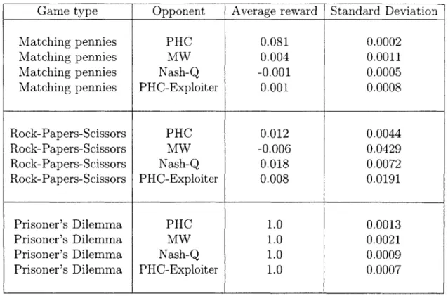
3.1 Summary of multi-agent learning algorithms under our new classifi-cation that categorizes algorithms by their observation history length and belief space complexity. . . . . 56 3.2 Table showing performance of the PHC-exploiter against different
op-ponents in various repeated games. Performance is given as average rewards per time period, over 20 trials. The game payoffs are given in F igure 2-1. . . . . 70 4.1 Table showing the mean, variance, skew, and kurtosis of the noise
distribution measured in the various experimental domains. . . . . 103 5.1 Comparison of the performance of the different methods for structuring
Chapter 1
Introduction
Learning enables us to adapt to the environment that surrounds us. By designing learning algorithms for robots and intelligent agents, we enable them to adapt to the environment into which we place them. This endeavor has produced many insights into the theory and practice of a single-agent learning to behave in a stationary envi-ronment. But what if the environment reacts to the agent? What if the environment includes opponents, or other agents? How do we need to change our learning methods to cope with a non-stationary or reactive environment?
Multi-agent learning captures an essential component of learning: the adaptivity of a learning agent to the environment around the agent. Often when we speak of learning in a single-agent domain, we implicitly assume that the environment is sta-tionary. Our main goal in this single-agent case is to find a good policy for operating in this stationary environment. Due to the environment's stationarity, the speed with which we learn becomes secondary in importance to the eventual convergence of our learning algorithm to a near-optimal solution. Accordingly, while many existing rein-forcement learning methods can be shown to find optimal policies in the limit, they are fairly slow to converge to this optimal policy.
In contrast, in multi-agent domains, the environment is assumed to change rapidly. Our opponents are part of the environment, and they may adapt to the way we act. They may indeed be trying to adapt to us as quickly as we are adapting to them. Thus, our learning algorithms must emphasize speed and adaptivity. This changes
the focus in the design of good multi-agent learning algorithms from convergence in the long run to good performance in the short run. The algorithms must adapt quickly but still be able to achieve good performance within some given amount of time.
1.1
Motivation
Bees dance to announce the finding of food. Ants count the number of run-ins with other ants to determine their best current role, be it forager, maintenance, or drone. Antelope congregate for safety from hunting lions. Chimpanzees can learn by ob-serving the mistakes of fellow chimps. And humans can acquire new behaviors by a variety of different means.
Whether these behaviors are learned or innate, they are invaluable for each species' survival in a world populated by a multitude of other animals. Either the species as a whole benefits from a cooperative behavior, or the individual benefits by avoiding a mistake committed by someone else or perhaps learning a new skill invented by someone else. While few people are prepared to call computer programs and robots a new species, various computer programs will eventually populate cyberspace, and increasingly sophisticated robots will begin to appear in the physical world around us. As a research community, we have thus far devoted most of our time creating intelligent agents or robots (henceforth called artificial agents, or simply agents) that can operate in various human-centric but static domains, whether directly helping humans in roles such as personal digital assistants or supporting human society in forms such as robotic assembly line manufacturers. However, as artificial agents become more prevalent and more capable, we may begin to see problems with this focus on the single agent. The interactions between all of the created agents will need to become a primary focus of our attention. The goals of the created agents may begin to conflict with one another, or we may begin to see the potential for cooperative behaviors amongst our agents.
delivering people or goods to prespecified locations. Most likely there will be some traffic information service that provides updates on traffic conditions for all of the possible routes for each vehicle. If all the vehicles acted selfishly, choosing the shortest route, the road system might experience bad oscillations in traffic volume. Ideally, we could enable the artificial agents in these scenarios to learn to cooperate with one another, settling on a policy of action that would be mutually beneficial. If we were a transit agency, our goal might be the overall efficiency of the entire regional road system. Or, if we were a luxury car manufacturer, our goal might be to design an agent with the single selfish aim of getting to its precious occupant to his or her destination as quickly as possible. Even in this case, the agent would have to rely on its prediction of the actions of all the other vehicles in the road network in order to achieve its desired goal. It could not operate as if the world were static, as if it were the only adaptive agent operating on the roads.
These are only two possible scenarios within the wide range of situations that might be encountered by a system of multiple agents. They are perhaps the most salient because it is easy to imagine that we will have to deal with these situations in the not-so-distant future. As such, these two scenarios represent the two main types of multi-agent systems we will explore further in this thesis. We call the second type "competitive, multi-designer systems" since the agents have conflicting goals and may be designed by many different individuals, each trying to create an agent that outsmarts all the others. In addition to purely competitive systems, we will also explore situations where coordination among the agents might lead to higher payoffs. The other type of situation is the "cooperative, single-designer system." In particular, we will explore complex cooperative systems that can be trained via simulation. They may or may not adapt further when actually deployed. The competitive agents, on the other hand, may or may not be trained prior to deployment, but will necessarily have to adapt their behavior in response to opponents once deployed and operating.
1.2
The approach
How do we begin studying such systems? Multi-agent domains are by their very nature highly complex. In order to study these domains, we need to pare them down to their bare essentials. One such setup is the repeated normal-form game. In this framework, the environment is the simplest it can be: a set of N x N matrices representing the rewards received by each agent, given a choice of actions by each agent. This allows us to focus on the game dynamics in terms of the interactions of the players, rather than their interaction with the environment. Most of the complexity will stem from the changing nature of the opponent, and the constant tension between trying to model and exploit the opponent while preventing the opponent from doing the same to us.
We will explore this framework in Chapter 3. Among other results, we will demon-strate that our beliefs about the types of opponents we are likely to face are very important for designing good algorithms. Some of this work was previously described by Chang and Kaelbling [2002].
1.3
Scaling up
From here, we try to increase the complexity of the environment, since it is hard to imagine repeated normal-form games finding wide applicability in real-world settings. Most real situations involve more complex environments that change as we act within them. Thus, our actions should affect the evolution of the environment state. In repeated normal-form games, we are always in the same state, playing the same normal-form game.
Furthermore, the environment is often too large for us to observe everything at once. If there are many agents operating in the same environment, we may not be able to observe what everyone is doing at the same time. Thus, we need methods that deal with this partial observability. Our approach is somewhat different from the traditional approach in the literature on partially observable Markov decision
processes (POMDPs), where methods have been developed to use memory to keep track of unobserved state variables. We also use a memory variable, but our main idea is to filter the reward signal so that a single agent is able to receive a training signal that is proportional to the credit that it is due. Thus, we do not explicitly track the states of the other agents, other than to maintain a single memory variable that summarizes the contribution of the rest of the system to the observed reward signal. Some of this work was previously described by Chang, Ho, and Kaelbling [2004a].
1.4
Highly complex domains
While the filtering approach provides us with a simple method for resolving multi-agent credit assignment in certain situations, its effectiveness is also limited. When the number of agents grows large, or if the agents are self-interested, the filtering approach cannot retrieve enough information from the observed reward signal to filter out a good training signal. Furthermore, the filtering method implicitly assumes that the environment, including the other agents, operates independently from the agent in question. In an adversarial domain, however, this is no longer the case, and thus the filtering approach would fail.
In such cases, we may need to develop a model of the world that explicitly in-cludes the other agents. The states and potential actions of all the agents in the system would have to be considered in order to estimate the value of an observed state from one agent's perspective. However, as Bernstein et al. [2002] have shown, even if we allow the agents to explicit communicate their partial state observations periodically, the decentralized control of a Markov decision process (MDP) is in-tractable. More specifically, in this case, it can be proved that there cannot be any polynomial-time algorithms to accomplish this task. Given this predicament, we need to resort to approximations or further assumptions in order to design algorithms (and thus agents) that perform reasonably well in such domains. Policy search is one such approximation [Peshkin et al., 2000].
opponent at all, then it is impossible to construct a learning algorithm that is optimal over all possible opponents. We must either restrict our attention to certain classes of opponents, or we must define a new notion of optimality. In this thesis, we introduce a new algorithm that approximates traditional optimal performance against large classes of opponents, and guarantees a regret bound against arbitrary opponents, which can be considered as a new notion of optimality.
We consider the potential for using experts that may be able to provide us with advice about which actions to perform. We might hope to resort to the advice of these experts to help us focus our search on potentially fruitful policies. The problem we then face is deciding between different expert advice. This framework can be used to derive a variety of different learning algorithms that provide interesting guarantees. In these combined learning algorithms, we can consider an individual learning algorithm to be one of the experts that provides us with advice from what it has learned thus far. We will call this approach hedged learning, since the algorithm hedges between following the various experts. For example, we present an algorithm that combines a set of given experts with an efficient MDP learner to create an algorithm that provides both a regret-minimizing guarantee and a polynomially time-bounded guarantee that it will find a near-optimal policy for the MDP.
Using experts provides us with a way of dealing with the adversarial, changing nature of the opponents in competitive settings. This framework is able to give us worst-case guarantees against such opponents. As long as we have decent experts to listen to, our performance is guaranteed to at least mimic the best expert closely and thus should be reasonably good. The importance of using these regret-minimizing techniques is that it insures that our learning process is in some sense hedged . That is, if one of our learning algorithms fails, we have intelligently hedged our bets between multiple different experts and thus we limit our losses in these cases. Some of this work is described by Chang and Kaelbling [2005].
1.5
A specialization: cooperative, single-designer
systems
We next study what seems to be the easier scenario: all of the agents are designed by a single architect, and all of the agents are working towards a single global goal. There is no longer a competitive issue caused by adversarial opponents. By limiting ourselves to systems where a single designer controls the entire system, we also do not need to consider interoperability issues and goal negotiation or communication amongst the agents. All of the agents know what the goal is and cooperate to achieve the goal.
Moreover, we might imagine that the designer is able to construct an approximate simulation of the world in which the agents are being designed to operate. These simulators could thus be used to train the agents before they are actually deployed in real situations. Flight simulators accomplish much the same task for human pilots.
We will introduce the mobilized ad-hoc networking domain as a basis for moti-vating our ideas on creating effective learning algorithms for cooperative multi-agent systems. This domain will also serve as a test-bed for our algorithms. Some of this work was previously described in Chang, Ho, and Kaelbling [2003].
1.5.1
Mobilized ad-hoc networking
Mobile ad-hoc networking is emerging as an important research field with a number of increasingly relevant real-world applications, ranging from sensor networks to peer-to-peer wireless computing. Researchers in Al and machine learning have not yet made major contributions this growing field. It promises to be a rich and interesting domain for studying the application of learning techniques. It also has direct appli-cations back to Al, for example in the design of communication channels for groups of robots. We introduce mobilized ad-hoc networks as a multi-agent learning domain and discuss some motivations for this study. Using standard reinforcement learning techniques, we tackled two distinct problems within this domain: packet routing and
node movement. We demonstrate that relatively straightforward adaptations of these methods are capable of achieving reasonable empirical results. Using the more so-phisticated techniques we develop in Chapter 5, we are able to improve upon this performance.
Mobile ad-hoc networks have not traditionally been considered a multi-agent learn-ing domain partly because most research in this area has assumed that we have no control over the node movements, limiting research to the design of routing algo-rithms. Each node is assumed to be attached to some user or object that is moving with its own purpose, and routing algorithms are thus designed to work well under a variety of different assumptions about node mobility patterns.
However, there are many applications in which we can imagine that some of the nodes would have control over their own movements. For example, mobile robots might be deployed in search-and-rescue or military reconnaissance operations requir-ing ad-hoc communication. In such cases it may be necessary for some nodes to adjust their physical positions in order to maintain network connectivity. In these situations, what we will term mobilized ad-hoc networks becomes an extremely rel-evant multi-agent learning domain. It is interesting both in the variety of learning issues involved and in its practical relevance to real-world systems and technology.
There are several advantages gained by allowing nodes to control their own move-ment. Stationary or randomly moving nodes may not form an optimally connected network or may not be connected at all. By allowing nodes to control their own movements, we will show that we can achieve better performance for the ad-hoc net-work. One might view these controllable nodes as "support nodes" whose role is to maintain certain network connectivity properties. As the number of support nodes in-creases, the network performance also increases. Given better movement and routing algorithms, we can achieve significant additional performance gains.
It is important to note that there are two levels at which learning can be applied: (1) packet routing and (2) node movement. We will discuss these topics in separate sections, devoting most of our attention to the more difficult problem of node move-ment. Packet routing concerns the forwarding decisions each node must make when
it receives packets destined for some other node. Node movement concerns the actual movement decisions each node can make in order to optimize the connectivity of the ad-hoc network. Even though we will use reinforcement learning techniques to tackle both these problems, they must each be approached with a different mind set. For the routing problem, we focus on the issue of online adaptivity. Learning is advanta-geous because it allows the nodes to quickly react to changes in network configuration and conditions. Adaptive distributed routing algorithms are particularly important in ad-hoc networks, since there is no centrally administered addressing and routing
system. Moreover, network configuration and conditions are by definition expected to change frequently.
On the other hand, the node movement problem is best handled off-line. Learning a good movement policy requires a long training phase, which would be undesirable if done on-line. At execution time, we should simply be running our pre-learned optimal policy. Moreover, this movement policy should encode optimal action selections given different observations about the network state; the overall policy does not change due to changing network configuration or conditions and thus does not need to adapt online. We treat the problem as a large partially-observable Markov decision process (POMDP) where the agent nodes only have access to local observations about the network state. This partial observability is inherent to both the routing and move-ment portions of the ad-hoc networking problem, since there is no central network administrator. Nodes can only observe the local state around them; they do not have access to the global network topology or communication patterns. Even with this limited knowledge, learning is useful because it would otherwise be difficult for a human designer to create an optimized movement policy for each network scenario.
Within this POMDP framework, we first attempt to apply off-the-shelf reinforce-ment learning methods such as Q-learning and policy search to solve the movereinforce-ment problem. Even though Q-learning is ill-suited to partially-observable domains, and policy search only allows us to find a locally optimal policy, we show that the re-sulting performance is still reasonable given a careful construction of the observation space. We then apply more sophisticated techniques that combine multiple learning
methods and predefined experts, resulting in much improved performance.
The packet routing and node movement problems represent two different methods for handling non-stationarity. In the case of packet routing, we allow the nodes to adapt rapidly to the changing environment. This type of fast, constant learning allows the nodes to maintain routing policies that work well, even though the environment is continuously changing. In the case of node movement, we take a different tack. We attempt to model the relevant aspects of the observed state space in order to learn a stationary policy. This stationary policy works well even though aspects of the environment constantly change, because we have modeled these changes in the policy's state space.
1.6
Thesis contributions
To summarize, this thesis presents new work in a diverse range of multi-agent settings. In the simplest repeated game setup, we present an analysis of the shortcomings of previous algorithms, and suggest improvements that can be made to the design of these algorithms. We present a possible classification for multi-agent algorithms, and we suggest new algorithms that fit into this classification.
In more complicated settings, we present a new technique that uses filtering meth-ods to extract a good training signal for a learning agent trying to learn a good reactive policy in a cooperative domain where a global reward signal signal is available. If the agent is given expert advice, we show that we can combine MDP learning algorithms with online learning methods to create an algorithm that provides online performance guarantees together with polynomially time-bounded guarantees for finding a near-optimal policy in the MDP.
If the setting is not cooperative, we cannot apply this filtering technique. We in-troduce the idea of hedged learning, where we incorporate knowledge about potential opponents in order to try to play well against as many possible opponents as possible. We show performance guarantees that can be obtained using this approach.
Chapter
2
Background
It comes as no surprise that there have been a wide range of proposed algorithms and models to tackle the problems we discussed in the previous chapter. One such framework, the repeated game, was first studied by game theorists and economists, and later it was studied by the machine learning community interested in multi-agent games. For more complex games, our use of filtering methods follows a long line of applications of filtering techniques for tracking underlying states of a partially observed variable. Regret-minimizing methods have been extensively studied by the online learning community, but have also been studied under different names such as universal consistency by the game theory community and universal prediction (and universal codes) by the information theory community. In this chapter, we provide background information on these diverse but very related fields.
2.1
Repeated games
Repeated games form the simplest possible framework for studying multi-agent learn-ing algorithms and their resultlearn-ing behavior. We first lay out the mathematical frame-work and provide an introduction to the basic definitions of game theory, then give a classification of prior work in the field of multi-agent learning algorithms. We then discuss some of the prior work developed within this framework, from both the game theory and machine learning perspectives.
2.1.1
Mathematical setup
From the game theory perspective, the repeated game is a generalization of the tradi-tional one-shot game, or matrix game. In the one-shot game, two players meet, choose actions, receive their rewards based on the simultaneous actions taken, and the game ends. Their actions and payoffs are often visually represented as a matrix, where action choices correspond to the rows or columns depending on the player executing the action, and payoffs are shown in the matrix cells. Specifically, the reward matrix Ri for each player i is defined as a function Ri : A1 x A2 -> R, where Ai is the set
of actions available to player i. As discussed, R1 is often written as an
IA
1 I x IA21matrix, with R1 (i, j) denoting the reward for agent 1 if agent 1 plays action i E A1
and agent 2 plays action j E A2. The game is described as a tuple (A1, A2, R1, R2) and is easily generalized to n players.
Some common (well-studied) examples of two-player, one-shot matrix games are shown in Figure 2-1. The special case of a purely competitive two-player game is called a zero-sum game and must satisfy R1 = -R 2.
In general, each player simultaneously chooses to play a particular pure action ai C Ai, or a mixed policy pi E PD(Ai), where PD(Ai) is the set of all possible probability distributions over the set of actions. The players then receive reward based on the joint actions taken. In the case of a pure action, the reward for agent i is given by Ri(ai, aj), and in the case of mixed policies, the reward is given as an
expectation, Ri(pi, ,pj) = E[Ri(ai, aj)jai ~ pi, aj - p]. For games where there are
more than two players, we will sometimes write the joint actions of all the other agents as a-i or [i.
The literature usually uses the terms policy and strategy interchangeably. As we will see later, sometimes policies or strategies will be more complicated mappings between states and action distributions.
The traditional assumption is that each player has no prior knowledge about the other player. Thus there is no opportunity to tailor our choice of action to best respond to the opponent's predicted action. We cannot make any predictions. As
is standard in the game theory literature, it is thus reasonable to assume that the opponent is fully rational and chooses actions that are in its best interest. In return, we would like to play a best response to the opponent's choice of action.
Definition 1 A best response function for player i, BRi(pi), is defined to be the set of all optimal policies for player i, given that the other players are playing the joint
policy pti: BRi(p-i) = {I p E MiIRi(p*, pi) > Ri(iI pi),Vpi E Mi}, where Mi is the set of all possible policies for agent i.
If all players are playing best responses to the other players' strategies, then the game is said to be in Nash equilibrium.
Definition 2 A Nash equilibrium is a joint policy p such that for every agent i,
pi C BRi
(p-i).-The fixed point result by Nash shows that every game must have at least one Nash equilibrium in mixed policies. Once all players are playing a Nash equilibrium, no single player has an incentive to unilaterally deviate from his equilibrium policy. Any game can be solved for its Nash equilibria using quadratic programming, and if the game only has a single Nash equilibrium, then a player can choose a strategy for playing against a similar, fully rational player in this fashion, given prior knowledge of the game structure. However, computing a Nash equilibrium is a computationally hard problem. To date there are no polynomial time algorithms for exactly solving a game to find all of its Nash equilibria, and it is an open question whether this problem is NP-hard [Papadimitriou, 2001].
A different problem arises when there are multiple Nash equilibria. If the players do not manage to coordinate on one equilibrium joint policy, then they may all end up worse off. The Hawk-Dove game shown in Figure 1(c) is a good example of this problem. The two Nash equilibria occur at (1,2) and (2,1), but if the players do not coordinate, they may end up playing a joint action (1,1) and receive 0 reward.
In the zero-sum setting, a fully rational opponent will choose actions that mini-mize our reward, since this in turn maximini-mizes its reward. This leads to the concept
R, =
R2= -R1]
(a) Matching pennies
R[0 R1= 1 23]
R2fl
0
]
(H D 3 2(c) Hawk-Dove, a.k.a. "Chicken"
0 -1 1 R, 1 0 -- 1 -1 1 0 R2=2-R (b) Rock-Paper-Scissors R [2 0 R1= 3 1 R2=[2 3 (d) = 0 1 (d) Prisoner's Dilemna
Figure 2-1: Some common examples of single-shot matrix games.
of minimax optimality, where we choose to maximize our reward given that the op-ponent is trying to minimize our reward. Von Neumann's minmax theorem proves the existence of an equilibrium point where both players are playing their minmax optimal strategies:
max min i 3 R,(pi, p) = min max j i R1 (Pi, P) -min max Rj 2 2(Pi, pj)
Traditionally, zero-sum games are also called "pure competitive" games. We use the term "competitive games" to include both pure, zero-sum games and general sum games where the agents have competing goals.
Minimax optimality in zero-sum games is a special case of Nash equilibrium in general-sum games. In general-sum games, we can no longer assume that the other player is trying to minimize our payoffs, since there are no assumptions about the relationship between the reward functions Ri. We must generally play a best response (BR) to the opponent's choice of action, which is a much harder question since we may be unable to predict the opponent's choice of action. We may need to know the
opponent's utility function Rj, and even if we know Rj, the opponent may or may not be acting fully rationally. Moreover, to complicate matters further, the set of opponent policies that can be considered "fully rational" will ultimately depend on the space of opponent types we are willing to consider, as we will discuss later.
2.1.2
Prior work
Nash equilibrium is commonly used as a solution concept for one-shot games. In contrast, for repeated games there are a range of different perspectives. Repeated games generalize one-shot games by assuming that the players repeat the matrix
game over many time periods. Researchers in reinforcement learning view repeated games as a special case of stochastic, or Markov, games. Researchers in game theory, on the other hand, view repeated games as an extension of their theory of one-shot matrix games. The resulting frameworks are similar, but with a key difference in their treatment of game history. Reinforcement learning researchers have most often focused their attention on choosing a single myopic stationary policy A that will maximize the learner's expected rewards in all future time periods given that
we are in time t, max, Ej
[z
1YR7-(p)] , where T may be finite or infinite, andp E PD(A). In the infinite time-horizon case, we often include the discount factor 0 < y < 1. We call such a choice of policy p myopic because it does not consider the effects of current actions on the future behavior of the opponent.
Littman [1994] analyzes this framework for zero-sum games, proving convergence to the Nash equilibrium for his Q algorithm playing against another
minimax-Q
agent. Claus and Boutilier [1998] examine cooperative games where R1 = R2, andHu and Wellman [1998] focus on general-sum games. These algorithms share the common goal of finding and playing a Nash equilibrium. Littman [2001] and Hall and Greenwald [2001] further extend this approach to consider variants of Nash equilib-rium, called correlated equilibria, for which convergence can be guaranteed.
When the opponent is not rational, it is no longer advantageous to find and play a Nash equilibrium strategy. In fact, given an arbitrary opponent, the Nash equilibrium strategy may return a lower payoff than some other action. Indeed, the payoff may
be even worse than the original Nash equilibrium value. For example, in the game of Hawk-Dove in Figure 2-1, one Nash equilibrium occurs when player 1 plays the first row action, and player 2 plays the second column action, leading to a reward of 3 for player 1 and a reward of 1 for player 2. However, if player 2 deviates and plays action 1 instead, they will both receive a reward of zero.
Even in zero-sum games, the problems still exists, though in a more benign form. As long as an agent plays a Nash equilibrium strategy, it can guarantee that it will receive payoff no worse than its expected Nash payoff, even if its opponent does not play its half of the Nash equilibrium strategy. However, even in this case, playing the Nash equilibrium strategy can still be suboptimal. For example, the opponent may not be playing a rational strategy. We would no longer need to worry about the mutual optimality condition of a Nash equilibrium; instead, we can simply play a best response to the opponent and exploit its irrationalities. Thus, in both general-sum and zero-sum games, we might hope that our agents are not only able to find Nash equilibrium strategies, but that they are also able to play best response strategies against non-Nash opponents.
Bowling and Veloso [2002b] and Nagayuki et al. [2000] propose to relax the mutual optimality requirement of Nash equilibrium by considering rational agents, which always learn to play a stationary best-response to their opponent's strategy, even if the opponent is not playing an equilibrium strategy. The motivation is that it allows our agents to act rationally even if the opponent is not acting rationally because of physical or computational limitations. Fictitious play [Fudenburg and Levine, 1995] is a similar algorithm from game theory.
Again, the goal is similar to the Nash approach: the agents should exhibit conver-gence to a stationary equilibrium, even if it is not the Nash equilibrium. Moreover, the agents should converge to a Nash equilibrium against a stationary Nash oppo-nent, but should be able to exploit any weaknesses of a non-Nash player. Indeed, Bowling and Veloso show that in games where there is a single Nash equlibrium, a special full-knowledge version of their WoLF-PHC algorithm converges to the Nash equilibrium when playing against itself.
2
3
6 7
Figure 2-2: This figure shows an example of a network game. There are seven players in this game, and the links between the players represent relationships between players that results in direct payoff consequences. For example, Player l's payoffs are only affected by its own actions, and the actions of Player 2 and Player 3. They are only indirectly affected by the action choices of the remaining four players, if Players 2 or Player 3's action choice is influenced by the rest of the players.
2.1.3
Solving for Nash equilibria
Recently there has been a great deal of interest in computational techniques for finding one or more Nash equilibria strategies for a given game. The general problem itself is usually quite difficult computationally, but it is an open question whether it is in P in the size of the game [Papadimitriou, 2001]. It is conjectured that the problem is somewhere between P and NP, since it is known to have at least one solution, unlike most problems that are NP-hard. However, new techniques take advantage of special structures in certain games to derive efficient computational techniques for finding Nash equilibria. For example, Littman et al. [2001] study network games, where a large game is structured into local interactions involving only small groups of agents. These local interactions may have effects that propagate throughout the network, but the immediate rewards of the local games are only directly observed by the local game participants. Figure 2-2 shows an example of a simple network game.
6-Player I Choice Node
Heads Tails
Player 2 Choice Node Player 2 Choice Node
Player 2's Information Set
Heads Tails Heads Tails
(1,-1) (-1,1) (-1,1) (1,-1)
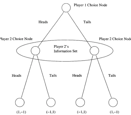
Figure 2-3: This figure shows the Matching Pennies game in extensive form. Clearly, the extensive form is a more general representation, since we can now allow the players to move sequentially and possess different information sets. Though not needed in this particular game, the extensive form representation can also include probabilistic choice nodes for "Nature", which can be used to account for randomness in the reward structure.
Nash equilibria in time polynomial in the size of the largest sub-game. Ortiz and Kearns [2002] extend this work to compute Nash equilibrium in loopy graphical games. Blum, Shelton, and Koller study a more general framework, described by multi-agent influence diagrams, or MAIDs [Blum et al., 2003]. The diagrams also graph-ically represent game structure, but they are richer descriptions than the network games studied by Kearns et al. MAIDs are able to capture information contained in extensive form games in a compact manner. Extensive form games generalize normal
form, or matrix, games by allowing the representation of sequential moves by the
var-ious players and different information sets available to the varvar-ious players. Extensive form games are usually represented as a tree, where branches of the tree represent
the different actions and agent may take from a particular node of the tree, (Figure 2-3). Blum et al. provide an algorithm that can compute an exact Nash equilibrium strategy in polynomial time.
2.1.4
Correlated Nash equilibria
For the sake of completeness, we will also mention the concept of a correlated Nash equilibrium. The correlated Nash equilibrium generalizes Nash equilibrium by allow-ing the players to coordinate, or correlate, their actions by observallow-ing a randomized external source of information. For example, consider this situation: two cars are approaching an intersection. If we assume that they must take simultaneous actions, then their Nash equilibrium would usually involve a randomized policy that chooses between the two possible actions, stop or go. However, if we add a traffic light to the intersection, then the cars can coordinate their actions based on the signal given by the traffic light. This would be a correlated Nash equilibrium.
It can be shown that if we force all the agents to use a particular learning algo-rithm, then the system will converge to a correlated Nash equilibrium [Greenwald and Hall, 20031. The intuition is that this learning algorithm uses the observed history of players' actions as the coordination signal.
2.1.5
Game theoretic perspective of repeated games
As alluded to earlier, modern game theory often take a more general view of opti-mality in repeated games. The machine learning community has also recently begun adopting this view [Chang and Kaelbling, 2002; de Farias, 2004]. The key differ-ence is the treatment of the history of actions taken in the game. Recall that in the stochastic game model, we took policies to be probability distributions over actions, pi E PD(A). We referred to this choice of policy as a myopic choice, since it did not consider the effects of the current policy on the future behavior of the opponent.
Here we redefine a policy to be a mapping from all possible histories of observations
set of all possible histories of length t. Histories are observations of joint actions, ht = (ai, a-i, h"l). Player i's strategy at time t is then expressed as pi(htl-).
We can now generalize the concept of Nash equilibrium to handle this new space of possible strategies.
Definition 3 Let ht be a particular sequence of actions that can be observed given that the agents are following policies pi and p-u. Given the opponent's policy Pa, a best response policy for agent i maximizes agent i's reward over the duration t of the game. We define the set of best response policies to be BRi(pi) =
{,p
EM tI = RT(p*,pi) Et= R'(pi,pi),Vpi E Mi}, where Mi is the set of all
pos-sible policies for agent i and R'(pi, p-i) is the expected reward of agent i at time
period T.
A Nash equilibrium in a repeated game that is repeated for t time periods is a joint strategy p(H) such that for every agent i, and every history of observations ht that
can be observed in the game given p(H), pi(ht) E BRi(pit(h t)).
For the infinitely repeated game, we let t -* oc. Now, the set of best response policies BRi(p_ ) becomes the set of all policies y4 such that
t t
lim sup J r-1R'(p, p-i) > lim sup T-1R'(pi, pi), Vpi E Mi,
t-o t-0 i
where 6 < 1 is a discount factor.
Let h be an infinite sequence of actions that can be observed given that the agents
are following policies pi and p_. A Nash equilibrium in the infinitely repeated game is a joint strategy p(H) such that for every agent i, and every history of observations
h' that can be observed in the game given p(H), pi(h) E BRl(pui(h)).
This definition requires that strategies be best responses to one another, where the earlier definition only required that simple probability distributions over action be best responses to one another. Henceforth, we will refer to the equilibrium in the earlier definition as a Nash equilibrium of the one-shot game. It is a stationary policy that is myopic.