Biogeochemical versus ecological
consequences of modeled ocean physics
The MIT Faculty has made this article openly available.
Please share
how this access benefits you. Your story matters.
Citation
Clayton, Sophie et al. “Biogeochemical Versus Ecological
Consequences of Modeled Ocean Physics.” Biogeosciences 14, 11
(June 2017): 2877–2889 © 2017 Author(s)
As Published
http://dx.doi.org/10.5194/BG-14-2877-2017
Publisher
Copernicus GmbH
Version
Final published version
Citable link
http://hdl.handle.net/1721.1/113856
Terms of Use
Attribution 3.0 Unported (CC BY 3.0)
https://doi.org/10.5194/bg-14-2877-2017 © Author(s) 2017. This work is distributed under the Creative Commons Attribution 3.0 License.
Biogeochemical versus ecological consequences
of modeled ocean physics
Sophie Clayton1,2, Stephanie Dutkiewicz1, Oliver Jahn1, Christopher Hill1, Patrick Heimbach1,3, and Michael J. Follows1
1Department for Earth, Atmospheric and Planetary Sciences, Massachusetts Institute of Technology, Cambridge, MA, USA 2School of Oceanography, University of Washington, Seattle, WA, USA
3Institute for Computational Engineering and Sciences and Jackson School of Geosciences,
The University of Texas at Austin, Austin, TX, USA Correspondence to:Sophie Clayton ([email protected])
Received: 14 August 2016 – Discussion started: 1 September 2016 Revised: 9 May 2017 – Accepted: 10 May 2017 – Published: 16 June 2017
Abstract. We present a systematic study of the differences generated by coupling the same ecological–biogeochemical model to a 1◦, coarse-resolution, and 1/6◦, eddy-permitting, global ocean circulation model to (a) biogeochemistry (e.g., primary production) and (b) phytoplankton commu-nity structure. Surprisingly, we find that the modeled phy-toplankton community is largely unchanged, with the same phenotypes dominating in both cases. Conversely, there are large regional and seasonal variations in primary production, phytoplankton and zooplankton biomass. In the subtropics, mixed layer depths (MLDs) are, on average, deeper in the eddy-permitting model, resulting in higher nutrient supply driving increases in primary production and phytoplankton biomass. In the higher latitudes, differences in winter mixed layer depths, the timing of the onset of the spring bloom and vertical nutrient supply result in lower primary produc-tion in the eddy-permitting model. Counterintuitively, this does not drive a decrease in phytoplankton biomass but re-sults in lower zooplankton biomass. We explain these sim-ilarities and differences in the model using the framework of resource competition theory, and find that they are the consequence of changes in the regional and seasonal nutri-ent supply and light environmnutri-ent, mediated by differences in the modeled mixed layer depths. Although previous work has suggested that complex models may respond chaotically and unpredictably to changes in forcing, we find that our model responds in a predictable way to different ocean circulation forcing, despite its complexity. The use of frameworks, such as resource competition theory, provides a tractable way to
explore the differences and similarities that occur. As this model has many similarities to other widely used biogeo-chemical models that also resolve multiple phytoplankton phenotypes, this study provides important insights into how the results of running these models under different physical conditions might be more easily understood.
1 Introduction
Ocean general circulation models have proved an invaluable tool for studying the role of phytoplankton in the global bio-geochemical cycles of climatically important elements. Re-cent advances have resulted in ever-higher-resolution physi-cal models of the ocean circulation (Menemenlis et al., 2008) and more complex ecological models incorporating larger numbers of phytoplankton functional groups and even indi-vidual phytoplankton phenotypes (Follows and Dutkiewicz, 2011). This trend for increasing resolution and complexity is aimed at creating model systems which incorporate some of the complexity seen in reality, with the hope of better re-solving biogeochemical processes. In this study we explore how differences in physical resolution affect, differently, the biogeochemistry and ecosystem of a coupled model.
The physical framework of an ocean model is fundamen-tal to accurately model biogeochemical cycles and phyto-plankton ecology (Doney, 1999; Anderson, 2005). Observa-tions have shown that phytoplankton biomass and commu-nity structure have characteristic temporal and spatial scales
corresponding most closely with the oceanic mesoscale and submesoscale (Platt, 1972; Strass, 1992; Abbott and Lete-lier, 1998; Doney et al., 2003; Cotti-Rausch et al., 2016). However, most global ocean models incorporating biogeo-chemical and ecological processes (especially those coupled in climate studies) do not resolve scales less than ∼ 1◦. In the ocean, the characteristic temporal and spatial scales of biology coincide with those of mesoscale and submesoscale physical dynamics. Spall and Richards (2000) showed in a high-resolution model of an unstable frontal jet that spatial heterogeneity in primary production occurred on scales of a few to tens of kilometers and that primary production could increase locally by up to 100 %. Coarse-resolution global biogeochemical models do not resolve these dynamics. Lévy (2008) and Mahadevan (2016) review the consequences of this for biogeochemical models. Previous studies have found that neglecting to resolve the mesoscale could result in errors of up to 30 % in the estimates of primary production (Lévy et al., 1998; Oschlies and Garçon, 1998; Mahadevan and Archer, 2000; McGillicuddy et al., 2003). Furthermore, Lévy et al. (2001) found discrepancies of up to 50 % in integrated primary production comparing a coarse-resolution model with one that resolved submesoscale dynamics. These studies found that, in the oligotrophic subtropical gyres, mesoscale (and submesoscale) dynamics drove an increased nutrient supply to the surface mixed layer, which enhanced rates of primary production. In the subpolar gyres, eddies appear to have a different effect on ocean biology. McGillicuddy et al. (2003) found in a 0.1◦-resolution model of the North Atlantic that mesoscale processes drove a geostrophic adjustment to deep winter convection, which reduced nutrient supply. How-ever, nutrients are less likely to be limiting than light in the subpolar gyres, so this may also have a positive effect on rates of primary production. Although these previous studies pre-dict the role of the mesoscale in modulating biological and biogeochemical responses in different regional settings, it is unclear what the integrated effect will be globally and what downstream effects might result.
The above studies, although they resolved higher-resolution physics, typically employed rather simple bio-geochemical models incorporating only one or two phyto-plankton functional types (PFTs). However, marine micro-bial communities are known to be incredibly diverse, and this diversity plays an important role in mediating global bio-geochemical cycles. Thanks to the continuing expansion of computing resources, diversity has been included in global biogeochemical models which resolve several phytoplank-ton functional groups (Chai et al., 2002; Gregg et al., 2003; Le Quéré et al., 2005), and even several tens of phytoplank-ton phenotypes within multiple functional groups have been developed (Follows et al., 2007; Ward et al., 2012). It is unknown whether a change in physical resolution will re-sult in any changes in the emergent community structure of one of these diverse models. Sinha et al. (2010) found that an intermediate-complexity ecosystem model which
re-solved five PTFs, run with two different physical models at a similar (coarse) resolution, could result in regional changes in the modeled phytoplankton communities. However, it is unclear whether the emergent community resulting from a more complex ecosystem model will be more or less robust to changes in the physical forcing.
Here we present a process study that explores the ef-fect of refining the physical resolution on a global, diverse ecosystem model which incorporates 78 distinct phytoplank-ton phenotypes. We explore both the effect on the bulk bio-geochemical properties and the community structure of the model solutions. The objective of this study is not to as-sess which model performs best with respect to reality or to suggest an optimal resolution. Rather, we aim to exam-ine how changes in the resolution and parameterization of subgrid scale processes of the model domain alter the emer-gent biogeochemical and ecological properties of this diverse ecosystem model and specifically to identify tools to help un-derstand these differences and similarities.
2 Method
This study is based upon numerical simulations of global ocean circulation, biogeochemical cycles and diverse phyto-plankton populations. We have employed the Massachusetts Institute of Technology General Circulation Model (MIT-gcm; Marshall et al., 1997) and biogeochemical and eco-logical model components as detailed in Dutkiewicz et al. (2009). Below, we describe these physical circulation and biogeochemical-ecological models in more detail.
2.1 Physical model configurations
We used two physical model configurations developed by the Estimating the Circulation and Climate of the Oceans (ECCO) project (Wunsch et al., 2009). Both span the pe-riod 1992–1999 and were constrained to be consistent with observed altimetry and hydrography. The high-resolution ECCO2 configuration, with an effective resolution of 1/6◦ and horizontal grid dimensions of ∼ 18 km (ECCO2; Men-emenlis et al., 2008), is referred to as eddy permitting, as it resolves large eddies at low latitudes, but remains below the first baroclinic Rossby radius at high latitudes (Chel-ton et al., 1998). We compare this high-resolution configu-ration with the ECCO–Global Ocean Data Assimilation Ex-periment state estimate (ECCO–GODAE, also referred to as ECCO version 3 in the lineage of ECCO production so-lutions; Wunsch and Heimbach, 2007, 2013), which has a coarser grid resolution of 1◦. Both physical models are data assimilation products. The ECCO–GODAE product is based on the Lagrange multiplier method, and the ECCO2 product employs a simplified Green’s function method. It should be noted that unlike most so-called ocean “reanalysis” products, both of the ECCO products are obtained using “smoother”
methods, which avoid the artificial adjustment motions that can be triggered during what is called “analysis increments” in data assimilative models which use “filtering” methods (Wunsch and Heimbach, 2013; Stammer et al., 2016). Be-cause the ECCO products are free of such artificial adjust-ments (expressed in particular in strong vertical adjustment motions that may confound vertical transport of biogeochem-ical tracers), they also conserve tracer and momentum bud-gets exactly.
A core focus of this study is comparing and contrast-ing the modeled ecological and biogeochemical behavior in a mesoscale eddy-permitting model (ECCO2) with a non-eddying model (ECCO–GODAE). Accordingly we limit our analysis latitudinally to the region between 60◦S and 60◦N. Within this latitudinal band, the first baroclinic radius of de-formation (Chelton et al., 1998) is larger than the ECCO2 model horizontal resolution, so the ECCO2 model admits corresponding mesoscale eddy dynamics. North and south of this latitude line, mesoscale eddies are not well resolved in either model, so neither model is in a so-called large-eddy regime (Smagorinsky, 1963). In the excluded high-latitude regions the two physical model mixed layers differ systemat-ically. These differences result from the absence of parame-terized mesoscale eddy dynamics in the ECCO2 model (Dan-abasoglu et al., 1994). This contrast in mixed layer depth, rather than behaviors due to mesoscale eddies, sets the dif-ferences in the biogeochemical response seen in ice-free high latitudes. For simplicity, we will refer to the ECCO–GODAE simulation as CR and the ECCO2 simulation as HR. 2.2 Ecological and biogeochemical model
The ecological model used in this study has previously been discussed in Follows et al. (2007) and Dutkiewicz et al. (2009). Briefly, we transport inorganic and organic forms of nitrogen, phosphorous, iron and silica, and resolve 78 phy-toplankton phenotypes and two simple grazers. The biogeo-chemical and biological tracers interact through the forma-tion, transformation and remineralization of organic matter. Excretion and mortality transfer living organic material into sinking particulate and dissolved organic detritus which are transpired back to inorganic form. The time rate of change in the biomass of each of the modeled phytoplankton types, Pj,
is described in terms of a light-, temperature- and nutrient-dependent growth, sinking, grazing, mortality and transport by the fluid flow. Many realizations of this ecological model, coupled to the ECCO–GODAE physical circulation, have been used to study a range of ecological questions, e.g., the role of top-down controls in setting patterns of phytoplank-ton diversity (Prowe et al., 2012; Vallina et al., 2014), the bio-geography of nitrogen-fixing phytoplankton (Monteiro et al., 2011) and role of transport in setting patterns in phytoplank-ton diversity (Clayphytoplank-ton et al., 2013).
In this study, the ecological model was initialized with 78 phytoplankton phenotypes with a broad range of
phys-iological attributes. Phytoplankton were assigned to one of two broad size classes by random draw at the initial-ization of the model, and a set of physiological trade-offs that reflect empirical observations were imposed ac-cordingly. We stochastically assigned plausible values for the nutrient half-saturation constants (κN), light and
tem-perature sensitivities within each phytoplankton functional group (Prochlorococcus-like, picophytoplankton, diatoms and large phytoplankton). Both the HR and CR simulations were initialized with an identical set of phytoplankton phe-notypes and initial conditions for all phytoplankton pheno-types, and in both cases the ecosystem model was forced with identical initial conditions for all variables, light forcing and dust inputs. Initial conditions for nutrients were taken from the January climatological values given in the World Ocean Atlas 2005 (Garcia et al., 2006). Interactions with the envi-ronment, competition with other phytoplankton, and grazing determine the composition of the phytoplankton communi-ties that persist in the model solutions.
We run both models for a total of 8 years, for the period from 1992 to 1999 from the same initial conditions. Although this is a relatively short run for a biogeochemical model, it currently would not be feasible to spin up the HR simula-tion for much longer. In several previous studies using the CR model (Dutkiewicz et al., 2009, 2012) and in this study for both CR and HR, we find that it takes only 3 years for the ecosystem to reach a stable annual cycle, so a run of 7– 8 years is sufficient to produce a repeating seasonal cycle in the modeled phytoplankton community. There was no dis-cernible trend in the globally integrated annual average phy-toplankton biomass in the last few years of either of the sim-ulations. The regional nutrient drifts that are linked to slow changes in the deep nutrient concentrations are small and sig-nificantly less than the seasonal and interannual variability.
We compare the model results for the last year (1999) from both model configurations to test the sensitivity of the ecosystem to the modeled ocean physics. The results of that comparison are described in the following section.
3 Results
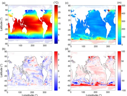
We describe differences in some of the physical properties most directly relevant to biogeochemical processes: sea sur-face temperature (SST) and mixed layer depth (MLD). Dif-ferences in other physical fields between the two model con-figurations have previously been discussed in Clayton et al. (2013); here we examine only those physical processes most directly relevant to biogeochemical processes not considered in that previous work. The SST patterns in both models are broadly similar, but we did find local differences in SST of up to 3◦C in some regions (Fig. 1). The HR simulation ap-peared to have a slight cool bias relative to the CR simu-lation, which is an indicator of enhanced upwelling and/or vertical mixing in the higher-resolution configuration. There
.
Figure 1. (a) Annual average sea surface temperature (SST) and (c) annual average mixed layer depths (MLD) in the HR simulation for the 1999 model year; (b) the difference in SST and (d) in MLD between the two simulations. Positive values indicate deeper MLD in the HR simulation, and negative values indicate deeper MLD in the CR simulation
were marked regional patterns in the MLD differences be-tween model configurations. Annual average MLDs were consistently deeper in the low latitudes in the HR simula-tion, whereas they tended to be slightly shallower in the mid-latitudes. As mentioned above, we exclude the high latitudes (> 60◦) from our analysis.
3.1 Primary production and biomass
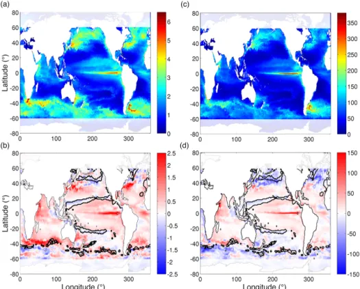
Both model configurations result in largely similar patterns in phytoplankton biomass and primary production, with low biomass and productivity associated with the subtropical gyres, and with higher biomass and productivity found in the mid-latitudes and upwelling zones. Although globally inte-grated primary production is very similar between both mod-els, with only a 0.6 % overall increase in primary produc-tion in the HR simulaproduc-tion, there are clear regional differences (Fig. 2), with higher rates of production in the low latitudes and lower rates of production in the mid-latitudes, in the HR simulation. We find a ∼ 20 % global increase in the stand-ing stock of phytoplankton biomass in the HR simulation, mostly accounted for by higher phytoplankton biomass be-tween 40◦S and 40◦N. The largest differences in both phyto-plankton biomass and primary production are associated with the western boundary currents and the equatorial upwelling zone, with higher values in the HR simulation. We also see decreases in phytoplankton biomass and productivity in the
HR simulation associated with the boundaries between dif-ferent biogeographical provinces.
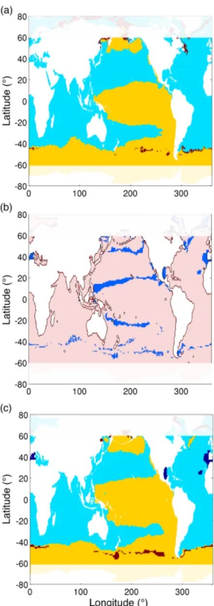
3.2 Phytoplankton community structure
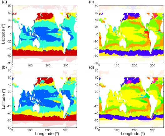
The ecological model represents a diverse community of phytoplankton, made up of individual phenotypes (analogous to species or ecotypes), which are defined by their nominal size, their nutrient requirements, their optimal light and tem-perature ranges, and their palatability to grazers. Each phy-toplankton phenotype belongs to one of four possible mod-eled phytoplankton functional groups. Phenotypes within each functional group have similar cell sizes and nutrient requirements but differ in their optimal light and tempera-ture ranges. To understand the impact of model resolution on the modeled phytoplankton community structure, we ex-amine the regional patterns in the dominant modeled phy-toplankton functional groups (Fig. 3a and b) and dominant modeled phytoplankton phenotypes (Fig. 3c and d). We find that the emergent phytoplankton community structure is re-markably similar between the two simulations. The low lati-tudes are dominated by Prochlorococcus analogues, whereas the mid-latitudes are dominated by diatoms and large phyto-plankton (Fig. 3a and b), with very little difference between models. What is even more striking, is that the regional pat-terns in the dominant phytoplankton phenotypes are largely unchanged between simulations. The only region that shows
Figure 2. (a) Annual average total phytoplankton biomass in g C m−2and (c) annual primary production in g C m−2yr−1in the HR model solution for 1999. (b) The difference in phytoplankton biomass and (d) the difference in annual primary production. Positive values indicate higher values in the HR simulation, and negative values indicate higher values in the CR simulation. The solid black contour lines in (b, d) indicate the region where the limiting nutrient differs between the two model simulations
a shift in the dominant functional group and phenotype be-tween model simulations is the Indian Ocean, which shifts from picophytoplankton dominated in the CR simulation to Prochlorococcus analogue dominated in the HR simula-tion, with a corresponding shift in the dominant phenotype. Other regions where the models do not agree occur mainly at the borders between different biogeochemical provinces. This suggests that changes in model resolution do not drive changes in the geographical range of dominant phenotypes, but this also suggests that they do not result in ecological shifts where different modeled phenotypes might become dominant. Given the big differences in modeled primary pro-duction and biomass described above, this is an unexpected result.
Differences in the patterns of phytoplankton biodiversity between the model simulations have previously been de-scribed in Clayton et al. (2013). Although we find an overall increase in phytoplankton biodiversity in the HR simulation (not shown here), those differences are mainly driven by the persistence of more rare species in the HR simulation with respect to CR and are thus unlikely to have a significant ef-fect on integrated bulk biogeochemical processes.
3.3 Nutrients and nutrient limitation
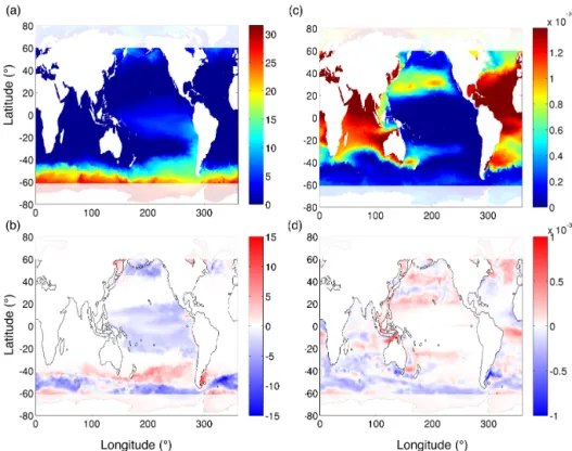
Differences in model resolution are expected to drive changes in the supply of nutrients to the surface photic zone. We do find differences in the concentration of surface macro-and micronutrients (Fig. 4). Nitrate macro-and dissolved iron both show marked patterns in the difference of their surface dis-tributions between simulations. The concentration of nitrate remains unchanged in the Atlantic, the Indian Ocean, and in some parts of the North and South Pacific (Fig. 4a). How-ever, there is a decrease in surface nitrate concentrations in the HR simulation in the mid-latitudes of the North Pacific and the Southern Ocean as well as in the subtropical and equatorial Pacific. Conversely, we see an increase in surface nitrate in the HR simulation in the Brazil–Malvinas Conflu-ence Zone and the region of the Subantarctic Front in the Southern Ocean. Differences in surface dissolved iron con-centrations exhibit markedly different patterns (Fig. 4b). The surface concentration of dissolved iron remains unchanged between model simulations in the subtropical and equatorial Pacific and parts of the subtropical North Atlantic. We see a general decrease in surface iron in the HR simulation in the Subantarctic Front in the Southern Ocean and the southern part of the Indian Ocean and an increase in dissolved iron in
Figure 3. Dominant phytoplankton functional group (a) in the HR simulation and (b) in the CR simulation. Diatoms are shown in red, large phytoplankton in yellow, picophytoplankton in green and Prochlorococcus-like phenotypes in blue. Dominant phytoplankton phenotype (c) in the HR simulation and (d) in the CR simulation. Each color represents a different phenotype.
the mid-latitudes of the North Pacific, the equatorial Atlantic, and the subpolar North Atlantic.
In addition to assessing the differences in surface nutrient concentrations, we determined the locally limiting nutrient for both models (Fig. 5). Nitrate and dissolved iron are the spatially dominant limiting nutrients in both model simula-tions, with almost identical regional patterns of limitation. However, we do find small but significant regions where the dominant limiting nutrients in both simulations do not corre-spond (Fig. 5b), primarily located at the boundaries between biogeographical provinces.
4 Discussion
In this study, we have assessed the effect of explicitly rep-resenting mesoscale dynamics in a global ocean ecological– biogeochemical model. Strikingly, we find that the realized phytoplankton communities in both simulations are remark-ably similar but that there are marked regional variations in bulk ecosystem properties such as primary production and phytoplankton biomass. We also find that although the general regional patterns of nutrient limitation remain un-changed, surface concentrations of nitrate and dissolved iron can vary markedly between simulations in some regions but are almost completely unchanged in others. Why do we see
such marked changes in the distribution of biogeochemical properties of the models but not in the modeled phytoplank-ton community? Here we explore what drives these similari-ties and differences, frequently using simple theoretical con-structs. The goal here is to provide a framework that other modellers can use to help understand some of the implica-tions of the physical–biogeochemical and ecological conse-quences of different forcings and resolutions.
Ultimately, any differences in the biogeochemical and eco-logical properties between the two model solutions occur ei-ther because ei-there are differences in the local physical fields (e.g., MLDs and transport) or because physical features of the ocean circulation such as the western boundary currents and gyre boundaries are realized in different locations. We identify three main regions that are affected in different ways by the addition of mesoscale dynamics: the tropical and sub-tropical regions, the subpolar gyres and the boundaries be-tween biogeographical provinces. We explore the linkages between the physical and biological components of the sys-tem to put these differences into context.
4.1 Tropical and subtropical regions
In the low latitudes, we found that the addition of mesoscale dynamics resulted in an overall deepening of the annual mean mixed layer depth (Fig. 1). We found an increase in
phyto-Figure 4. Annual average surface concentrations of (a) nitrate in mmol N m−3and (c) dissolved iron in mmol Fe m−3in the HR model solution for model year 1999; (b) the difference in nitrate and (d) the difference in dissolved iron. Positive values indicate higher values in the HR simulation, and negative values indicate higher values in the CR simulation.
plankton biomass and primary production, but the dominant phytoplankton functional group and phenotypes remained unchanged. The increase in primary production and phyto-plankton biomass in the HR simulation was not entirely sur-prising, as it has been predicted by previous regional and ide-alized studies on the effect of increasing model resolution on primary production (Lévy et al., 2001; Oschlies and Garçon, 1998; Mahadevan and Archer, 2000; Spall and Richards, 2000; McGillicuddy et al., 2003). However, we may have expected a large increase in the biomass of large phytoplank-ton thanks to more episodic eddy-driven nutrient injections to the surface mixed layer, as observed by Benitez-Nelson et al. (2007) and Brown et al. (2008). In fact, the increase in phytoplankton biomass was driven by an increase in the abundance of the dominant phytoplankton functional groups, Prochlorococcus analogues and picophytoplankton, which are both small, gleaner types. We also found that where a particular nutrient was limiting in both model simulations, its surface concentration remained unchanged.
The subtropical gyres are steady, stable regions where sea-sonality is low and phytoplankton growth is nutrient limited. In this context, we can apply the simple resource competi-tion framework introduced by Tilman et al. (1982) and ap-plied to this system by Dutkiewicz et al. (2009) to understand the simultaneous differences and similarities in the model re-sults. We set up a simple model system, where phytoplank-ton growth is nutrient limited and balanced by a simple linear
mortality term: dR dt = − µMAXRP R + k +SR, (1) dP dt = µMAXRP R + k −mP , (2)
where R is the limiting resource, P is the phytoplankton biomass, µ is the maximum phytoplankton growth rate, k is the resource half-saturation constant, m is the phytoplankton mortality rate and SRis the rate of resource supply into the
system. The steady state solution for this system is P∗=SR
m, (3)
R∗= mk
µ − m. (4)
In this framework, the steady state concentration of the lim-iting resource, R∗, is controlled not by the magnitude of
the nutrient supply but by the physiological attributes of the dominant phytoplankton phenotype. In this type of sta-ble system, the emergent dominant phytoplankton phenotype will be the one that can draw the resource down to the low-est R∗value. As we have set the phytoplankton communities to be composed of the same phenotypes in both simulations, and R∗is set by the physiological traits of the phytoplankton (Dutkiewicz et al., 2009), we select for the same dominant
Figure 5. Limiting nutrients were assessed based on a biomass weighted average of the most limiting nutrient for each of the 78 total phytoplankton types (a) in the HR model and (c) in the CR model. Iron-limited regions are shown in orange, nitrate-limited in light blue, phosphate-limited in dark blue and silica-limited in red. (b) Regions where the model simulations predict different limiting nutrients are shown in dark blue, whereas pink regions have the same limiting nutrient in both simulations.
phenotype in both simulations. Conversely, the steady state concentration of the phytoplankton, P∗, is a function of the resource supply, SR, as well as the mortality rate. Thus, an
increase in SR results in increased phytoplankton biomass,
but not in a shift in the dominant phytoplankton type, as R∗ is only a function of the physiology of the fittest phytoplank-ton type. Enhanced mixing in the HR simulation drives an increase in SRbut does not change the dominant
phytoplank-ton phenotype. Rather, it results in an increase in the biomass of the dominant type and an increase in productivity (µP∗). At the same time, the concentration of the limiting nutrient,
R∗, remains unchanged (as seen in nitrate and dissolved iron, Fig. 4), but the non-limiting nutrients decrease due to in-creased removal by the inin-creased productivity (Fig. 4). This may also result in a decrease in the supply of resources down-stream from the subtropical gyres.
For instance, we see a dramatic increase in phytoplankton biomass and primary production in the equatorial region of the HR model simulation. We evaluated the annual average vertical advective flux of nitrate (wNO3) at 100 m between
5◦N and 5◦S for both models. The regionally integrated mean annual vertical nitrate fluxes evaluated at 100 m for model year 1999 were 453.1 and 383.7 mmol NO3m−2yr−1
for the HR and CR simulations, respectively. There is a clear increase in vertical nutrient supply in the equatorial up-welling zone in HR that can account for the dramatic increase in phytoplankton stock and primary productivity in the equa-torial Pacific.
4.2 Subpolar regions
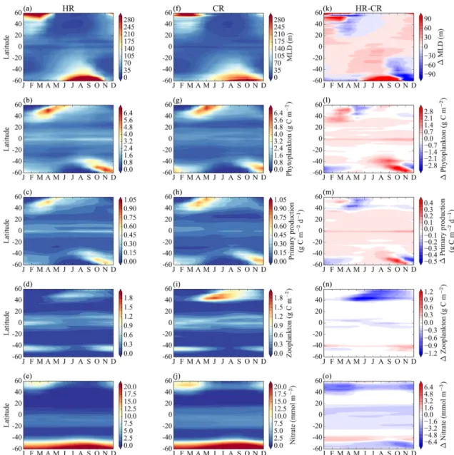
We see a somewhat different picture in the mid- to high lat-itudes, where there is an overall decrease in annual mean primary production, and to a lesser degree in phytoplank-ton biomass in HR compared to CR (Fig. 2). Again, the dominant phytoplankton functional groups and phenotypes remain largely unchanged between models in these regions (Fig. 3). What is most striking is the much higher abundance of zooplankton found in the northern subpolar gyres of the CR model solution (Fig. 6). In order to explain these dif-ferences, we must look more closely at the evolution of the seasonal cycle in both models (Fig. 6).
First we consider the different behaviors of the models during the winter months. HR has deeper mixed layer depths from November through March or April, depending on lati-tude. During this period, higher light limitation explains the lower primary production levels. In the context of this model, the limiting factors on the phytoplankton growth rate are multiplicative – e.g., for each modeled phytoplankton phe-notype j , the growth term is given by
µj=µMAXjγjTγjI
R R + kRj
, (5)
where γT and γI are the temperature and light limitation terms, respectively. During the winter, when nutrients are re-plete (and the nutrient limitation term approaches 1), if either the light or temperature fields experienced by the modeled phytoplankton are consistently less favorable, then µ will be decreased. Consistently deeper winter MLDs in the HR sim-ulation during the winter months result in lower winter pri-mary production in HR than CR.
The onset of the spring bloom occurs roughly 1 month earlier (March–April) in the HR simulation than in the CR simulation (April–May). This is reflected in the higher pri-mary production in the HR simulation in March and April, followed by a reversal with higher primary production in the
Figure 6. Hovmöller diagram showing the seasonal evolution of zonally averaged model properties for the HR simulation (left column), the CR simulation (middle column) and their difference (right column). First row: mixed layer depth; second row: phytoplankton biomass; third row: primary production; fourth row: zooplankton biomass; fifth row: surface nitrate concentration. The difference is calculated as HR − CR, so positive values indicate larger values in the HR simulation.
CR simulation in May. This is driven by differences in the timing of the shoaling of the MLDs, which occurs earlier in the HR model due to the action of mesoscale eddies.
During the summer and into the early autumn, the shal-lower mixed layer depths restrict nutrient resupply and nu-trients become limiting. As the physical and biogeochemi-cal properties of both models are relatively stable over sev-eral months during the summer period, we represent them as an idealized steady state system (see e.g., Dutkiewicz et al., 2009, Fig. 4) to better understand the processes driving the differences between the two models. In these higher lati-tudes, grazer dynamics become uncoupled from their prey. Thus we construct an idealized model system similar to
Eqs. (1) and (2) but that now includes explicit grazing by zooplankton. dR dt = −µMAX RP R + k+SR, (6) dP dt =µMAX RP R + k−gZP , (7) dZ dt =gZP − mzZ, (8)
where R is the resource, P is the phytoplankton biomass, µMAX is the maximum phytoplankton growth rate, k is the
nutrient half-saturation constant, g is the grazing rate of phy-toplankton by zooplankton, mzis the zooplankton mortality
rate and SRis the rate of resource supply into the system. The
steady state solution for this system is R∗= kSRg −gSR+µMAXmz , (9) P∗=mz g , (10) Z∗=k( SRg µMAXmz −1). (11)
For this system, P∗, the phytoplankton standing stock, is controlled by the physiological traits of the zooplankton which are constant, so regardless of changes in SR
phyto-plankton biomass will remain the same. However, Z∗, the
zooplankton standing stock, is directly proportional to SR, so
increased nutrient supply results in higher zooplankton abun-dance. Applying this framework to our model results, we are able to explain the increase in zooplankton biomass, the roughly unchanged phytoplankton biomass and the increased primary production in CR compared to HR. In contrast to the situation during the winter, in this case it is driven primar-ily by differences in nutrient supply. We evaluated the annual mean vertical nitrate supply by advection, which was 142.1 and 108.1 mmol NO3m−2yr−1in CR and HR, respectively.
That, coupled with the deeper summer MLDs in CR, results in an increased nutrient supply compared to HR. Zhang et al. (2013) find a similar response to nutrient injections at a shelf break front, where increases in primary production are fun-neled up the trophic levels and result in increased zooplank-ton biomass but are not reflected in increased phytoplankzooplank-ton biomass. On a larger scale, Ward et al. (2012) found in a global, size-structured ecosystem model that, in regions of higher nutrient supply, top-down control drives an increase in the biomass of larger plankton size classes relative to olig-otrophic regions rather than an unchecked increase in smaller size classes. Similar patterns can be seen in the Southern Hemisphere, where the MLD shoals earlier in the spring in the HR simulation, and primary production and phytoplank-ton biomass are both lower in the HR simulation during the summer.
4.3 Boundaries between biogeographical provinces We found marked differences in biological fields which ap-pear to be due to differences in the geographical extent of biogeographical provinces between simulations. Differences in modeled phytoplankton biomass and primary production in the North and South Pacific subtropical gyres coincide exactly with geographical differences in regions defined by different limiting nutrients in the simulations (Fig. 2). We attribute this decrease in production and biomass to a de-crease in the lateral supply of nutrients from the equatorial upwelling region. This decreased lateral supply out of the equatorial region in the HR simulation is due to more lo-cal primary production in the equatorial region (Fig. 2). Al-though dissolved iron is drawn down to the same
concentra-tion in both simulaconcentra-tions, primary producconcentra-tion and phytoplank-ton biomass are higher, and nitrate is much lower in the HR simulation. As discussed above, resource competition the-ory predicts that the concentration of the limiting nutrient, R∗(in this case dissolved iron; Fig. 5), is unchanged when the phytoplankton community remains unchanged. Increased dissolved iron supply associated with deeper MLDs would drive the increase in primary production and phytoplankton biomass observed in the in the HR simulation. However, this increase in local primary production, consuming higher lev-els of non-limiting macronutrients locally, reduces the Ek-man transfer of non-limiting nutrients to the neighboring sub-tropical gyres (Dutkiewicz et al., 2005). A similar shift in bi-ological transition zones, associated with model resolution, was found in a regional study of the California Current sys-tem. Fiechter et al. (2014) found that increasing the resolu-tion of their model from 1/3 to 1/30◦ resulted in a marked
shift in the location of the transition between nearshore out-gassing and offshore absorption of CO2. These differences in
gas fluxes were driven, in their study, by different patterns in nutrient upwelling and transport offshore.
4.4 Stability of the phytoplankton community structure
As we have discussed in the previous sections, one of the most striking results of our model comparison is that de-spite the difference in the modeled physics, the emergent phytoplankton communities in both simulations are almost identical. We only know of one comparable study where the response of a complex ecosystem model to different model physics has been evaluated (Sinha et al., 2010). In that study, although there was a difference in resolution between the two physical models used to force the ecosystem model (1◦vs. 2◦), unlike our study, both of these physical models were too coarse to resolve eddies. Although the physical models in the (Sinha et al., 2010) study were initialized and forced in es-sentially the same way, they were run out without being con-strained to observations. This resulted in large differences in their model solutions for physical fields (e.g., seasonal SST, see their Fig. 3), which were used to force the ecosystem model. One very key difference in our study with respect to the earlier work of Sinha et al. (2010) is that both of the physical models used to force our ecosystem model, ECCO– GODAE and ECCO2, were state estimates constrained to converge as closely as possible to observational data. Al-though the state estimates were constrained in different ways, and differences between them remain, compared to free-running models without any assimilation, these differences are comparatively small. In the end, the differences in the ECCO state estimates used in this study are largely a conse-quence of whether or not they represent mesoscale dynamics.
5 Conclusions
In this study we have compared and contrasted the behavior of a complex ecological–biogeochemical model when cou-pled to either a mesoscale eddy-permitting high-resolution physical model (HR, ECCO2) or a non-eddying coarse-resolution physical model (CR, ECCO–GODAE). We found that increasing the model resolution to include mesoscale dy-namics does not greatly affect the structure of our modeled phytoplankton ecosystem. However it does have a significant effect on the regional distribution of the bulk properties of the ecosystem: primary production and phytoplankton and zooplankton biomass. We have used theoretical constructs to help us pull apart the reasons for these differences and simi-larities.
One of the most striking results of this study is the ro-bustness of the emergent modeled phytoplankton commu-nity. We found that the dominant phytoplankton functional groups and phenotypes remained unchanged between simu-lations, despite differences in SST and MLDs. In contrast, we found marked regional differences in phytoplankton and zooplankton biomass and in primary production. By apply-ing concepts from resource competition theory (Tilman et al., 1982; Dutkiewicz et al., 2009), we can explain why in the subtropical gyres, despite increased primary production, the dominant phytoplankton phenotype and the surface concen-tration of the limiting nutrient remain the same in both sim-ulations. The combination of low seasonality and low graz-ing pressure means that despite an increased nutrient supply, phytoplankton with the lowest R∗will always be selected for in this region. Conversely, deeper winter and shallower sum-mer MLDs in the HR model, along with differences in the timing of the spring shoaling of the MLD, result in lower primary production and lower zooplankton biomass in HR than in the CR model.
Given the complexity of our ecosystem model, which in-corporates 78 individual phytoplankton types, it may seem surprising that our modeled phytoplankton community struc-ture is so similar in both cases. This presents interesting im-plications for marine biogeochemical and ecological model-ing. It is clear that accuracy in the representation of the phys-ical dynamics of the environment is necessary for effectively modeling ocean biogeochemistry. The higher taxonomic res-olution of our ecological model may in fact allow for subtler gradations of change in the phytoplankton community when the environment is changed, whereas in coarser ecological models regime shifts could easily result due to larger dif-ferences between modeled phenotypes. We do not advocate simply tuning parameters to get the “right” result, but rather increasing the physiological parameter space constrained by laboratory and observational work in order to create a more robust and representative model of the phytoplankton com-munity.
We have shown that the bulk biogeochemical properties of this ecological model are more sensitive to differences
in modeled ocean physics than the structure of the ecosys-tem itself. Given that this model has many similarities to other widely used biogeochemical models, which also re-solve multiple phytoplankton PFTs, this study provides im-portant insights into how these models might behave un-der different physical conditions. Our results show that the physics resolved by the models do matter, regardless of the scope of the question being addressed. The modeled MLD plays a central role in mediating bulk biogeochemical pro-cesses, specifically through vertical nutrient supply and the modulation of the light environment, which ultimately con-trol the magnitude of bulk biological rate processes. Notably, although global values of primary production, and to a lesser extent phytoplankton biomass, are similar between models, the bulk biogeochemical properties of the model solutions differ regionally. This shows that regardless of whether one is interested in global or regional questions, model resolution is crucially important.
It may be tempting to conclude from the results pre-sented here that, in fact, model resolution is less important when considering ecological problems. However, we would strongly caution against this as although we have shown that the dominant constituents of the phytoplankton community remain largely unchanged regardless of model resolution, significant differences in phytoplankton productivity, diver-sity (Clayton et al., 2013) and overall community composi-tion do result from differences in model resolucomposi-tion.
We have shown in this study that, even for complex eco-logical models, it is possible to explain differences in model solutions, and a similar approach could be taken to evaluate the effect of different model physics on different ecological model formulations.
Data availability. Due to the large volume of the model output data used in this study, we are unable to make it publicly available. How-ever, the corresponding author is happy to provide selected model fields upon request. The modeling framework used in this study, MITgcm, can be downloaded from http://mitgcm.org.
The Supplement related to this article is available online at https://doi.org/10.5194/bg-14-2877-2017-supplement.
Author contributions. Sophie Clayton, Stephanie Dutkiewicz and Michael J. Follows designed the study. Stephanie Dutkiewicz, Oliver Jahn, Patrick Heimbach and Christopher Hill implemented and ran the model simulations. Sophie Clayton analyzed the model outputs. Sophie Clayton prepared the manuscript with contributions from all coauthors.
Competing interests. The authors declare that they have no conflict of interest.
Acknowledgements. We thank Dennis McGillicuddy and Amala Mahadevan for helpful discussions on this work and three anonymous reviewers whose comments improved the manuscript. This study was funded by grants from the National Science Foundation (OCE-1434007 and OCE-1048897), the Gordon and Betty Moore Foundation, and the Simmons Collab-oration on Ocean Processes and Ecology. Sophie Clayton was funded by a Moore/Sloan Data Science and Washington Research Foundation Innovation in Data Science post-doctoral fellowship at the University of Washington. Patrick Heimbach was supported through NASA’s Physical Oceanography program.
Edited by: C. P. Slomp
Reviewed by: three anonymous referees
References
Abbott, M. R. and Letelier, R. M.: Decorrelation scales of chloro-phyll as observed from bio-optical drifters in the California Cur-rent, Deep-Sea Res. Pt. II, 45, 1639–1667, 1998.
Anderson, T.: Plankton functional type modelling: running before we can walk?, J. Plankton Res., 27, 1073–1081, 2005.
Benitez-Nelson, C. R., Bidigare, R. R., Dickey, T. D., Landry, M. R., Leonard, C. L., Brown, S. L., Nencioli, F., Rii, Y. M., Maiti, K., Becker, J. W., Bibby, T. S., Black, W., Cai, W.-J., Carlson, C. A., Chen, F., Kuwahara, V. S., Mahaffey, C., McAndrew, P. M., Quay, P. D., Rappé, M. S., Selph, K. E., Simmons, M. P., and Yang, E. J.: Mesoscale eddies drive increased silica export in the subtropical Pacific Ocean, Science, 316, 1017–1021, 2007. Brown, S., Landry, M., Selph, K., Jin Yang, E., Rii, Y., and
Bidi-gare, R.: Diatoms in the desert: Plankton community response to a mesoscale eddy in the subtropical North Pacific, Deep-Sea Res. Pt. II, 55, 1321–1333, 2008.
Chai, F., Dugdale, R., Peng, T., Wilkerson, F., and Barber, R.: One-dimensional ecosystem model of the equatorial Pacific upwelling system. Part I: model development and silicon and nitrogen cy-cle, Deep-Sea Res. Pt. II, 49, 2713–2745, 2002.
Chelton, D. B., Deszoeke, R. A., Schlax, M. G., El Naggar, K., and Siwertz, N.: Geographical variability of the first baroclinic Rossby radius of deformation, J. Phys. Oceanogr., 28, 433–460, 1998.
Clayton, S., Dutkiewicz, S., Jahn, O., and Follows, M. J.: Disper-sal, eddies, and the diversity of marine phytoplankton, Limnol-ogy and Oceanography: Fluids and Environments, 3, 182–197, https://doi.org/10.1215/21573689-2373515, 2013.
Cotti-Rausch, B. E., Lomas, M. W., Lachenmyer, E. M., Gold-man, E. A., Bell, D. W., Goldberg, S. R., and Richardson, T. L.: Mesoscale and sub-mesoscale variability in phytoplankton com-munity composition in the Sargasso Sea, Deep-Sea Res. Pt. I, 110, 106–122, 2016.
Danabasoglu, G., McWilliams, J., and Gent, P.: The role of mesoscale tracer transports in the global ocean circulation, Sci-ence, 264, 1123–1125, 1994.
Doney, S. C.: Major challenges confronting marine biogeochemical modeling, Global Biogeochem. Cy., 13, 705–714, 1999. Doney, S. C., Glover, D. M., McCue, S. J., and Fuentes,
M.: Mesoscale variability of Sea-viewing Wide Field-of-view Sensor (SeaWiFS) satellite ocean color: Global
pat-terns and spatial scales, J. Geophys. Res.-Oceans, 108, 3024, https://doi.org/10.1029/2001JC000843, 2003.
Dutkiewicz, S., Follows, M. J., and Parekh, P.: Interactions of the iron and phosphorus cycles: A three-dimensional model study, Global Biogeochem. Cy., 19, GB1021, https://doi.org/10.1029/2004GB002342, 2005.
Dutkiewicz, S., Follows, M. J., and Bragg, J. G.: Mod-eling the coupling of ocean ecology and biogeo-chemistry, Global Biogeochem. Cy., 23, GB4017, https://doi.org/10.1029/2008GB003405, 2009.
Dutkiewicz, S., Ward, B. A., Monteiro, F., and Follows, M.: In-terconnection of nitrogen fixers and iron in the Pacific Ocean: Theory and numerical simulations, Global Biogeochem. Cy., 26, GB1012, https://doi.org/10.1029/2011GB004039, 2012. Fiechter, J., Curchitser, E. N., Edwards, C. A., Chai, F., Goebel,
N. L., and Chavez, F. P.: Air-sea CO2fluxes in the California
Cur-rent: Impacts of model resolution and coastal topography, Global Biogeochem. Cy., 28, 371–385, 2014.
Follows, M. J. and Dutkiewicz, S.: Modeling diverse communities of marine microbes, Annu. Rev. Mar. Sci., 3, 427–451, 2011. Follows, M. J., Dutkiewicz, S., Grant, S., and Chisholm, S. W.:
Emergent Biogeography of Microbial Communities in a Model Ocean, Science, 315, 1843–1846, 2007.
Garcia, H., Locarnini, R., Boyer, T., Antonov, J., and Levitus, S.: World Ocean Database 2005, Volume 4: Nutrients phosphate, ni-trate, silicate [+ DVD], NOAA Atlas NESDIS, 2006.
Gregg, W., Ginoux, P., Schopf, P., and Casey, N.: Phytoplankton and iron: validation of a global three-dimensional ocean biogeo-chemical model, Deep-Sea Res. Pt. II, 50, 3143–3169, 2003. Le Quéré, C., Harrison, S. P., Prentice, I. C., Buitenhuis, E. T.,
Au-mont, O., Bopp, L., Claustre, H., Cunha, L. C. D., Geider, R., Gi-raud, X., Klaas, C., Kohfeld, K. E., Legendre, L., Manizza, M., Platt, T., Rivkin, R. B., Sathyendranath, S., Uitz, J., Watson, A. J., and Wolf-Gladrow, D.: Ecosystem dynamics based on plankton functional types for global ocean biogeochemistry models, Glob. Change Biol., 11, 2016–2040, 2005.
Lévy, M.: The Modulation of Biological Production by Oceanic Mesoscale Turbulence, in: Transport and Mixing in Geophysical Flows, Vol. 744, p. 219, Springer Berlin Heidelberg, 2008. Lévy, M., Mémery, L., and Madec, G.: The onset of a bloom after
deep winter convection in the northwestern Mediterranean sea: mesoscale process study with a primitive equation model, J. Ma-rine Syst., 16, 7–21, 1998.
Lévy, M., Klein, P., and Tréguier, A.-M.: Impact of sub-mesoscale physics on production and subduction of phytoplankton in an oligotrophic regime, J. Mar. Res., 59, 535–565, 2001.
Mahadevan, A.: The impact of submesoscale physics on primary productivity of plankton, Annu. Rev. Mar. Sci., 8, 161–184, 2016.
Mahadevan, A. and Archer, D.: Modeling the impact of fronts and mesoscale circulation on the nutrient supply and biogeochem-istry of the upper ocean, J. Geophys. Res., 105, 1209–1225, 2000.
Marshall, J., Hill, C., Perelman, L., and Adcroft, A.: Hydrostatic, quasi-hydrostatic, and nonhydrostatic ocean modeling, J. Geo-phys. Res., 102, 5733–5752, 1997.
McGillicuddy, D., Anderson, L., Doney, S., and Maltrud, M.: Eddy-driven sources and sinks of nutrients in the upper ocean: Results from a 0.1 resolution model of
the North Atlantic, Global Biogeochem. Cy., 17, 1035, https://doi.org/10.1029/2002GB001987, 2003.
Menemenlis, D., Campin, J., Heimbach, P., Hill, C., Lee, T., Nguyen, A., Schodlok, M., and Zhang, H.: ECCO2: High res-olution global ocean and sea ice data synthesis, Mercator Ocean Quarterly Newsletter, 31, 13–21, 2008.
Monteiro, F., Dutkiewicz, S., and Follows, M.: Biogeographical controls on the marine nitrogen fixers, Global Biogeochem. Cy., 25, GB2003, https://doi.org/10.1029/2010GB003902, 2011. Oschlies, A. and Garçon, V.: Eddy-induced enhancement of primary
production in a model of the North Atlantic Ocean, Nature, 394, 266–269, 1998.
Platt, T.: Local phytoplankton abundance and turbulence, in: Deep Sea Research and Oceanographic Abstracts, 19, 183–187, https://doi.org/10.1016/0011-7471(72)90029-0, Elsevier, 1972. Prowe, A. E. F., Pahlow, M., and Oschlies, A.: Controls on the
diversity-productivity relationship in a marine ecosystem model, Ecol. Model., 225, 167–176, 2012.
Sinha, B., Buitenhuis, E. T., Le Quere, C., and Anderson, T. R.: Comparison of the emergent behaviour of a complex ecosystem model in two ocean general circulation models, Prog. Oceanogr., 84, 204–224, 2010.
Smagorinsky, J.: General circulation experiments with the primitive equations: I. the basic experiment∗, Mon. Weather Rev., 91, 99– 164, 1963.
Spall, S. and Richards, K.: A numerical model of mesoscale frontal instabilities and plankton dynamics – I. Model formulation and initial experiments, Deep-Sea Res. Pt. I, 47, 1261–1301, 2000. Stammer, D., Balmaseda, M., Heimbach, P., Köhl, A., and Weaver,
A.: Ocean data assimilation in support of climate applications: status and perspectives, Annu. Rev. Mar. Sci., 8, 491–518, 2016.
Strass, V. H.: Chlorophyll patchiness caused by mesoscale up-welling at fronts, Deep-Sea Res. Pt. A, 39, 75–96, 1992. Tilman, D., Kilham, S., and Kilham, P.: Phytoplankton community
ecology: the role of limiting nutrients, A. Rev. Ecol. Syst., 13, 349–372, 1982.
Vallina, S. M., Ward, B. A., Dutkiewicz, S., and Follows, M. J.: Maximal feeding with active prey-switching: A kill-the-winner functional response and its effect on global diversity and bio-geography, Prog. Oceanogr., 120, 93–109, 2014.
Ward, B. A., Dutkiewicz, S., Jahn, O., and Follows, M. J.: A size-structured food-web model for the global ocean, Limnol. Oceanogr., 57, 1877, https://doi.org/10.4319/lo.2012.57.6.1877, 2012.
Wunsch, C. and Heimbach, P.: Practical global oceanic state esti-mation, Physica D, 230, 197–208, 2007.
Wunsch, C. and Heimbach, P.: Dynamically and kinematically con-sistent global ocean circulation and ice state estimates, in: Ocean Circulation and Climate: A 21 Century Perspective, Elsevier, 2013.
Wunsch, C., Heimbach, P., Ponte, R. M., Fukumori, I., and Mem-bers, T. E.-G. C.: The Global General Circulation of the Ocean Estimated by the ECCO-Consortium, Oceanography, 22, 88– 103, https://doi.org/10.5670/oceanog.2009.41, 2009.
Zhang, W. G., McGillicuddy, D. J., and Gawarkiewicz, G. G.: Is biological productivity enhanced at the New England shelfbreak front?, J. Geophys. Res.-Oceans, 118, 517–535, 2013.