Publisher’s version / Version de l'éditeur:
Vous avez des questions? Nous pouvons vous aider. Pour communiquer directement avec un auteur, consultez la première page de la revue dans laquelle son article a été publié afin de trouver ses coordonnées. Si vous n’arrivez pas à les repérer, communiquez avec nous à PublicationsArchive-ArchivesPublications@nrc-cnrc.gc.ca.
Questions? Contact the NRC Publications Archive team at
PublicationsArchive-ArchivesPublications@nrc-cnrc.gc.ca. If you wish to email the authors directly, please see the first page of the publication for their contact information.
https://publications-cnrc.canada.ca/fra/droits
L’accès à ce site Web et l’utilisation de son contenu sont assujettis aux conditions présentées dans le site LISEZ CES CONDITIONS ATTENTIVEMENT AVANT D’UTILISER CE SITE WEB.
ASHRAE Transactions [Proceedings], pp. 1-17, 2008-06-21
READ THESE TERMS AND CONDITIONS CAREFULLY BEFORE USING THIS WEBSITE.
https://nrc-publications.canada.ca/eng/copyright
NRC Publications Archive Record / Notice des Archives des publications du CNRC :
https://nrc-publications.canada.ca/eng/view/object/?id=60d4d75a-7a08-435f-b37b-102cc8e6ee21 https://publications-cnrc.canada.ca/fra/voir/objet/?id=60d4d75a-7a08-435f-b37b-102cc8e6ee21
NRC Publications Archive
Archives des publications du CNRC
This publication could be one of several versions: author’s original, accepted manuscript or the publisher’s version. / La version de cette publication peut être l’une des suivantes : la version prépublication de l’auteur, la version acceptée du manuscrit ou la version de l’éditeur.
Access and use of this website and the material on it are subject to the Terms and Conditions set forth at
Summer and winter field monitoring of high and low solar heat gain
glazing at a Canadian twin house facility
Manning, M. M.; Elmahdy, A. H.; Swinton, M. C.; Parekh, A.; Szadkowski, F.;
Barry, C.
http://irc.nrc-cnrc.gc.ca
S u m m e r a n d w i n t e r f i e l d m o n i t o r i n g o f h i g h
a n d l o w s o l a r h e a t g a i n g l a z i n g a t a
C a n a d i a n t w i n h o u s e f a c i l i t y
N R C C - 5 0 2 6 9
M a n n i n g , M . M . ; E l m a h d y , A . ; S w i n t o n , M . C . ;
P a r e k h , A . ; S z a d s k o w s k i , F . ; B a r r y , C .
A version of this document is published in / Une version de ce document se trouve dans: ASHRAE Transactions, Salt Lake City, Utah, June 21-25, 2008, pp. 1-17
The material in this document is covered by the provisions of the Copyright Act, by Canadian laws, policies, regulations and international agreements. Such provisions serve to identify the information source and, in specific instances, to prohibit reproduction of materials without written permission. For more information visit http://laws.justice.gc.ca/en/showtdm/cs/C-42
Les renseignements dans ce document sont protégés par la Loi sur le droit d'auteur, par les lois, les politiques et les règlements du Canada et des accords internationaux. Ces dispositions permettent d'identifier la source de l'information et, dans certains cas, d'interdire la copie de documents sans permission écrite. Pour obtenir de plus amples renseignements : http://lois.justice.gc.ca/fr/showtdm/cs/C-42
Summer and Winter Field Monitoring
of High and Low Solar Heat Gain
Glazing at a Canadian Twin House
Facility
M.M. Manning, A. Elmahdy, M.C. Swinton – National Research Council Canada A. Parekh, F. Szadskowski – Natural Resources Canada
C. Barry – Pilkington North America, Inc. ABSTRACT
During the winter heating season of 2005-2006 and the summer cooling season of 2006, a series of tests were conducted to determine the impact of spectrally selective coated glass on energy consumption at a Canadian twin R-2000 house facility. Two low-emissivity (low-e) coatings were compared on a whole house basis: a high solar heat gain glazing and a low solar heat gain glazing technology. In addition to impact on energy consumption, differences in room temperatures, window surface temperatures, and the transmission of solar radiation were evaluated. Correlations between incident vertical solar radiation and consumption were developed and used to predict annual consumption and to compare the potential savings from the two technologies. This paper presents the results from these field tests and presents the methodology and the results from this analytical projection. A seperate accompanying paper addresses the use of these results to refine computer simulation tools, and describes the energy analysis of these glazing systems for a range of North American climate zones.
INTRODUCTION
Windows and other types of fenestration systems are key components of all types of buildings. On the energy performance, windows play a dual role, allowing solar gains to offset the auxiliary heating loads during the heating season or add to building loads during the cooling season. Various research studies have shown that, in a typical Canadian house with the conventional windows, the window heat losses during the heating season account for more than 40% of total heat losses. The solar gains typically range from 10% to 27% of total energy requirements for the house. During the summer months, excessive solar gains through windows add to cooling loads. During the last two decades, significant research efforts have resulted in the development of high thermal performance, low emissivity coated glass in windows. The products available today have generally much better insulating values; however, many may have lower solar heat gains.
The actual solar heat gain through the glazing system is greatly affected by the solar/optical characteristics of the coating on the glass. Knowledge of the actual coating performance is essential in setting energy targets and extracting information to determine the impact of the high efficient windows on energy rating, load management, and reduction of space heating load as well as reduction of the cooling load demand.
With rising cooling loads and associated peak electric demands in large population centers, there is a need to optimize the selection of windows in houses which can provide greater overall energy efficiency during the heating season along with better solar control during the summer months.
The project consisted of two components: a) a field evaluation of two different glazing technologies at the twin house facility during heating and cooling seasons, and b) a computer simulation to calibrate models, and to perform an extensive energy analysis of various types of glazing units for the different climate zones. This paper presents the full results of the field study including both winter and summer results, as well as an analytical extrapolation of results to the full year. Details from the winter field tests were published by Swinton et al., 2007. Detailed results from the computer simulations are presented in the accompanying paper (Parekh in press).
Testing was conducted in a unique facility consisting of identical two-storey R-2000* houses in Ottawa, Canada. These twin houses feature an energy efficient passive solar design, a simulated occupancy program, and are fully instrumented with over 300 sensors. Since its launch in 1998, the facility has been the site of many energy-related side-by-side evaluations of heating and cooling technologies. Evaluated technologies include: natural gas-fired combo systems (Swinton et al. 2000), the electronically commutated motor (Gusdorf et al. 2003), indoor and outdoor blinds (Galasiu et al. 2005), and thermostat setback (Manning et al. 2007).
OBJECTIVES
The primary objective of the field testing was to compare the thermal performance of two advanced glazing systems, and to quantify their impact on the overall space heating and cooling requirements of the house. A secondary objective was to identify the differences in performance characteristics of the glazing units themselves in terms of solar transmission to the house, night heat losses and changes in window surface temperatures.
The output of this project will serve multiple purposes including: the quantification of heat gain/loss through glazing systems; the refinement of computational tools used to determine the energy rating of windows; the benchmarking of “high performance” vs “conventional windows”; support of the development (and/or refinement) of national and international standards on energy rating of windows; and the development of design guidelines for optimizing the energy and peak power demand performance for appropriate selection and installation of innovative window systems in different climates.
EXPERIMENTAL SETUP
Description of the Twin Houses
The twin houses are located at the government run Canadian Centre for Housing Technologyin Ottawa, Ontario, Canada. The houses are built to R-2000 standards and feature an energy efficient passive solar design. House specifications are listed in Table 1. In addition to these features, the houses include a simulated occupancy system that simulates the daily actions of a family of four, including water draws (250 L [66 gal.] hot water/day) and electrical loads for lighting and appliances (9 kWh/day non HVAC loads). The internal heat gains from the occupants are also simulated, through the use of 60 W (adult) and 40 W (children) light bulbs.
Table 1. Research House Specifications
Feature Details
Construction Standard R-2000
Liveable Area 210 m2 (2260 ft2), 2 storeys
Insulation Attic: RSI 8.6 (R-49), Walls: RSI 3.5 (R-20), Rim joists: RSI
3.5 (R-20)
Basement Poured concrete, full basement
Floor: Concrete slab, no insulation
Walls: RSI 3.5 (R-20) in a framed wall. No vapour barrier.
Garage Two-car, recessed into the floor plan; isolated control room in
the garage
Exposed floor over the garage RSI 4.4 (R-25) with heated/cooled plenum air space between
insulation and sub-floor.
Windows Area: 35.0 m2 (377 ft2) total, 16.2 m2 (174 ft2) South Facing
Air Barrier System Exterior, taped fiberboard sheathing with laminated weather
resistant barrier. Taped penetrations, including windows.
Airtightness 1.6 air changes per hour @ 50 Pa (1.0 lb/ft2)
Furnishing Unfurnished
*
Description of the Glazing Technology
High Solar Heat Gain (HSG). In the benchmark configuration, both the Test House and the Reference house were glazed with high solar heat gain (HSG), Chemical Vapour Deposition (CVD) coated low emissivity, sealed double glazed units (rated centre of glass U-Factor = 1.65 W/m2°K [0.29
Btu/hr.ft2.°F], rated centre of glass SHGC = 0.72, rated window U-factor = 1.76 W/m2°K [0.31
Btu/hr.ft2.°F], rated window SHGC = 0.52).
Low Solar Heat Gain (LSG). In the experimental configuration, the Reference House was left in Benchmark condition (unchanged) and the Test house was re-glazed with a low solar heat gain (LSG), low emissivity, sputter-coated low emissivity glass, sealed double glazed units (rated center of glass U-Factor = 1.36 W/m2°K [0.24 Btu/hr.ft2.°F], rated centre of glass SHGC = 0.41, rated window U-factor = 1.62
W/m2°K [0.29 Btu/hr.ft2.°F], rated window SHGC = 0.33).
Approach
The field assessment of glazing technology took place in two sets of tests: winter assessment in January/February 2006 and summer assessment in July 2006. A side-by-side testing approach was used, as outlined by Swinton et al. (2001). For each season, the houses were initially “benchmarked” in identical configuration with the HSG glazing units installed in all windows of boths houses, in order to identify small differences in house performance. Following an initial period of benchmarking, all glazing units were switched to LSG technology in one of the houses, referred to as the “Test House”. The second house, referred to as the “Reference House”, remained in the benchmark configuration with HSG windows. A second period of benchmarking and airtightness testing occurred following the experiment to ensure that house performance remained unchanged.
The winter test included a total of 13 benchmark days before the experiment, 28 experiment days (19-Jan-06 to 15-Feb-06), and 10 benchmark days following the experiment. During the winter experiment period, outdoor temperature ranged from –18.6°C (-1.5°F) to 7.5°C (45.5°F). Daily solar radiation incident
on the south face of the house ranged from 1205 kJ/m2/day (106.1 Btu/ft2/day) to 22599 kJ/m2/day (1990.0
Btu/ft2/day). Temperature conditions on winter benchmarking days ranged from -18.9°C (-2.0°F) to 15.9°C
(60.6°F). Total daily vertical solar radiation on the south face ranged from 871 kJ/m2/day (77.7
Btu/ft2/day) to 21905 kJ/m2/day (1928.8 Btu/ft2/day).
The summer test included a total of 9 benchmark days before the experiment, 23 experiment days (7-Jul-06 to 1-Aug-06), and 15 benchmark days following the experiment. During the summer experiment period, outdoor temperatures ranged from 11.3°C (52.3°F) to 33.3°C (91.9°F). Daily solar radiation
incident on the south face of the house ranged from 3520 kJ/m2/day (310.0 Btu/ft2/day) to 12136 kJ/m2/day
(1068.6 Btu/ft2/day). This is much lower than the winter values, which reached 22599 kJ/m2/day (1990.0
Btu/ft2/day). The low position of the sun in the sky during the winter months causes more radiation to
strike the south face of the house. Temperature conditions on summer benchmarking days ranged from 7.6°C (45.7°F) to 30.0°C (86.0°F). Total daily vertical solar radiation on the south face ranged from 1693
kJ/m2/day (149.1 Btu/ft2/day) to 13426 kJ/m2/day (1182.2 Btu/ft2/day).
Data Collection
During winter testing, summer testing, and benchmarking alike, a number of parameters were monitored:
Solar radiation. A precision spectral pyranometer mounted on the south-facing brick wall of the Reference House measured total global solar radiation on the vertical plane. A second identical pyranometer was mounted behind the south-facing window of the Test House bedroom 2. Pyranometer
measurements, in W/m2, were recorded on a 5-minute basis and daily totals, in kJ/m2/day, were calculated
for the analysis. The difference between the readings of the two pyranometers was used as an indication of the transmission properties of the window. The pyranometers’ measurements can not be seen as an absolute measurement of transmission, as the field of view of the window-mounted pyranometer is obstructed partially by the surrounding window. However, this measurement was used to compare the two sets of windows – during benchmarking, and during the experiment.
Furnace Consumption. In each house, an electric meter with pulse output measured the furnace circulation fan electrical consumption and a gas meter with pulse output measured the furnace natural gas consumption. Measurements were recorded on a 5-minute basis, at a resolution of 0.0006 kWh/pulse, and
0.05 ft3/pulse respectively. Daily totals for both electrical and gas consumption were used in the analysis.
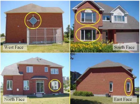
Window Surface Temperatures. Window surface temperatures were monitored at one exterior and three interior locations on each window by thermocouples mounted to the window surface using a thermally conductive epoxy. The accuracy of temperature measurements was +/- 0.1°C. A total of five windows were instrumented – two on the south face of the building, and one window on each of the north, east, and west faces. Figure 1 shows photos of all four faces of the research house. Instrumented windows are circled.
Airtightness Testing. A standard blower door test was performed prior to and following the window experiment in both summer and winter. This was done to verify that the houses maintained their airtightness despite changes to the envelope (window replacement). The airtightness of the houses were measured using the blower door tests according to CGSB 149.10 test procedure in the ‘as operating’ conditions. During the winter and summer testing, even with the replacement of glazing units in the Test house, the airtightness levels in both Reference and Test houses differed slightly. The associated air leakage
heat loss difference is minimal. During winter testing, the air change rates at 50 Pa (1.0 lb/ft2) for the
houses were: 1.61 air changes per hour (ACH) for the Reference House, and 1.57 ACH for the Test House.
Equivalent leakage areas (ELA) at 10 Pa (0.2 lb/ft2) were 599 cm2 (92.8 in2) and 584 cm2 (90.5 in2)
respectively. During summer testing, the air change rates at 50 Pa (1.0 lb/ft2) were: 1.63 ACH for the
Reference House, and 1.60 ACH for the Test House. ELA’s at 10 Pa (0.2 lb/ft2) were 590 cm2 (91.5 in2)
and 604 cm2 (93.6 in2) respectively.
Room Temperatures. Room air temperatures were recorded hourly in each of four south-facing rooms: livingroom, bedroom 2, master bedroom and ensuite; at three different heights: ceiling level, mid height and floor level. The accuracy of temperature measurements was +/- 0.1°C.
Figure 1. Four orientations of the Research House, showing instrumented window locations Mechanical Equipment
A single centrally located programmable thermostat controlled both the space heating and cooling systems. Features of the thermostat included: a 2°C (4°F) nominal deadband, and a cycle rate of 3 cycles/hr when at the 50% load condition. The thermostat setting for winter tests was 22°C (72°F), and
was chosen as the operating condition to satisfy the needs of a number of winter experiments at the facility. The summer thermostat setting was 26°C (79°F). This setting was chosen in accordance to ASHRAE standard 90.2-2004, which designates the summer temperature setting at 25.6°C (78°F).
Both houses were equipped with a high efficiency condensing gas furnace @ 94% steady state efficiency (measured) with a standard permanent split capacitor (PSC) motor. The furnace motor operated in low-speed continuous circulation when not providing high-speed distribution for space heating or cooling. The rated output of the furnace was 71.2 MJ/h (67,500 Btu/h). A 13 SEER (nominal) air conditioning unit with 2 ton capacity provided cooling. A heat recovery ventilator (HRV) @ 84%
efficiency (nominal) operated at low speed (1.8 m3/min [65 cfm] ) continually throughout all winter tests.
A different HRV was installed for the summer as part of a facility upgrade, and operated at 80% efficiency (nominal), and was operated at 62 cfm continually. Hot water heating was provided by a conventional, induced draft water heater @ 67% efficiency (measured).
Air is distributed throughout the house via sheet metal ducting. Supply registers and air returns are located on all three floors: nine supply registers, and two return grilles on the first floor; 11 supply registers and five return grilles on the second floor; and three supply registers and a single return grille in the basement. Air is supplied at approximately 570 L/s (1200 cfm) in heating mode and in air conditioning mode, and 280 L/s (600 cfm) in continuous circulation, as per the furnace motor’s standard operating speeds.
Analysis
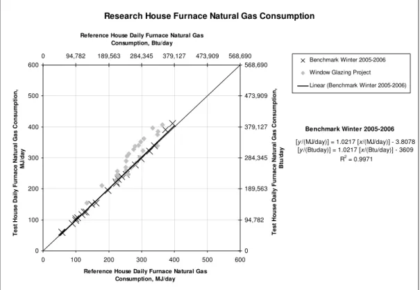
Consumption. Furnace natural gas and electrical consumption and air conditioner electrical consumption were compiled on a daily basis from 5-minute data. By plotting the daily consumption of the Test House vs the Reference House, trends were developed for the benchmark and experiment across a range of environmental conditions (see Figure 2 for an example). Using the Reference House consumption as a reference, the benchmark line correlation was used to calculate the amount of energy consumed by the Test House with the HSG windows for any given day of the experiment. Daily savings were determined by comparing the Test House consumption with LSG windows to the calculated Test House consumption under benchmark conditions. The advantage of using the Reference House as a reference, instead of depending on correlations with outdoor temperature, is that both houses are exposed to identical outdoor conditions. This allows the effects of the windows to be isolated from wind, solar and temperature effects.
Room and Surface Temperatures. A similar strategy was used to analyze the effect of the window glazing on room and surface temperatures. Again, by plotting the daily maximum temperature of the Test House vs the Reference House, trends were developed for the benchmark. Using the Reference House maximum temperature as a reference, the benchmark line correlation was used to calculate the maximum expected temperature in the Test House with HSG windows. The change in temperature due to the LSG windows was determined by comparing the maximum measured temperature for a given day in the Test House with LSG windows, to the calculated Test House maximum temperature under benchmark conditions.
Solar Transmission. During benchmarking, a correlation was developed between the total daily vertical solar radiation, and the total incident solar radiation behind the HSG window. Using the total daily vertical solar as a reference, the benchmark correlation was used to calculate the expected total solar radiation incident on the pyranometer mounted behind an HSG window on experiment days. The reduction in transmitted solar radiation was then calculated by taking the difference between the measured transmission behind the LSG window, and the calculated transmission in benchmarking configuration (behind an HSG window). Correlations were developed between the change in consumption due to the LSG windows, the total daily global solar radiation on the vertical plane and the reduction in transmission. RESULTS
Consumption
During the winter experiment, furnace natural gas consumption was monitored in both houses. The resulting daily consumption data is plotted along side the benchmarking data in Figure 2. Total daily
Reference House furnace gas consumption is plotted on the x-axis, while total daily Test House furnace gas consumption is plotted on the y-axis. Each point represents a single day of data. By plotting multiple days, a trend can be developed to indicate the relative performance of the two houses. If the two houses were in fact perfectly identical, the benchmark would have a slope of 1 and intercept at 0. There are always small differences between the houses, as it is impossible for them to be completely identical. This is seen by the slightly higher slope, and intercept that is less than 1.
On average, the results show an increase in gas consumption due to the installation of the LSG windows. The average increase over the duration of the winter glazing experiment was 23.9 MJ/day (22,700 Btu/day), with a maximum increase of 61.5 MJ/day (58,300 Btu/day). Over the entire experimental period in the winter, the increased consumption associated with the LSG technology was 8.7% for gas and 1.3% for electricity.
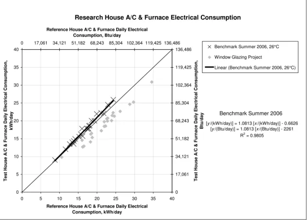
Similar trends were developed for the summer experiment data. Both the summer benchmark and experiment data for daily air conditioning electrical consumption (including air conditioner compressure and furnace circulation fan electrical consumption) are plotted in Figure 3. Again, the benchmark trendline is not perfect, small differences exist between the houses and their air conditioning systems, which are taken into account in the analysis.
On average, the results show a decrease in cooling system electrical consumption due to the installation of the LSG windows. The average decrease over the duration of the summer glazing experiment was 14.8 MJ/day (14,000 Btu/day), with a maximum decrease of 22.5 MJ/day (21,300 Btu/day). Over the entire experimental period in the summer, the reduction in cooling consumption associated with the LSG technology was 17.7%.
The large amount of scatter in the glazing experiment data during both the winter and summer tests can be related directly to solar radiation. On days with high amount of solar radiation, the differences between the windows have greater impact, and the experiment point is further away from the benchmark trend line. On days with low amounts of solar radiation, points are much closer to the benchmark trend, and on a few occasions are below the benchmark line. The relationship between solar radiation and consumption data is further explored later in the next sections.
Research House Furnace Natural Gas Consumption
[y /(MJ/day)] = 1.0217 [x/(MJ/day)] - 3.8078 [y /(Btuday)] = 1.0217 [x/(Btu/day)] - 3609 R2 = 0.9971 0 100 200 300 400 500 600 0 100 200 300 400 500 600
Reference House Daily Furnace Natural Gas Consumption, MJ/day
Test House Daily Fur
nace Natur a l G as Consumption, MJ /d a y 0 94,782 189,563 284,345 379,127 473,909 568,690 0 94,782 189,563 284,345 379,127 473,909 568,690
Reference House Daily Furnace Natural Gas Consumption, Btu/day
Test House Daily Fur
nace Natur a l G as Consumption, Btu/day Benchmark Winter 2005-2006 Window Glazing Project
Linear (Benchmark Winter 2005-2006)
Benchmark Winter 2005-2006
Research House A/C & Furnace Electrical Consumption [y /(kWh/day)] = 1.0813 [x /(kWh/day)] - 0.6626 [y /(Btu/day)] = 1.0813 [x /(Btu/day)] - 2261 R2 = 0.9805 0 5 10 15 20 25 30 35 40 0 5 10 15 20 25 30 35 40
Reference House A/C & Furnace Daily Electrical Consumption, kWh/day
Test
House A/
C & Furnace Dai
ly E lect ri cal Consumpt ion, kWh/ day 0 17,061 34,121 51,182 68,243 85,304 102,364 119,425 136,486 0 17,061 34,121 51,182 68,243 85,304 102,364 119,425 136,486
Reference House A/C & Furnace Daily Electrical Consumption, Btu/day
Test
House A/
C & Furnace Dai
ly E lect ri cal Consumpt ion, Bt u/ day Benchmark Summer 2006, 26°C Window Glazing Project
Linear (Benchmark Summer 2006, 26°C)
Benchmark Summer 2006
Figure 3. Summer Air Conditioning Electrical Consumption
Solar Transmission
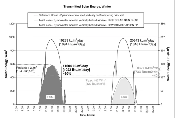
The most notable difference between the two types of glazing is their ability to transmit solar radiation. This difference is demonstrated in Figure 4. Two days of winter solar data are plotted in this graph:
January 15th – a Benchmark day, and January 26th – an Experiment day. On January 15th, a pyranometer
was mounted behind a south-facing HSG window. On January 26th, the pyranometer was situated at the
same south-facing location, behind a LSG window. Only 40% of the total solar radiation incident on a wall with the same orientation as the window was detected behind the LSG window. Whereas, on the sample benchmark day, 60% of the solar radiation was transmitted by the HSG window. (These numbers do not include the energy absorbed, convected and radiated to the room).
On days with low solar gains, where less than 4000 kJ/m2/day (352.2 Btu/ft2/day) were incident on the
south face of the house, the relationship between percentage of transmitted solar energy and total solar energy breaks down. On these days, the percentage of solar energy transmitted by the windows dropped for both the LSG and HSG windows. This result demonstrates that on days with low solar gains, generally very cloudy days, the spectrally selective properties of the low emissivity coating associated with the two different technologies are of less importance.
Two days of summer solar data are plotted in Figure 5. In terms of transmission, the summer results differ greatly from the winter results. In winter, not only was the amount of transmitted solar energy higher (57% on average for HSG and 40% for LSG windows), but the percentage of transmitted energy was also constant across a large range of incident solar radiation. In the summer, the percentage of solar energy transmitted by the window dropped with increased incident solar radiation. In the case of the LSG
windows, transmission was highest ~40% on days with less than 5000 kJ/m2/day (440.3 Btu/ft2/day)
vertical solar radiation, and dropped to ~32% on the clearest days of the experiment.
The explanation for this difference between summer and winter transmission is linked to the angular properties of glass. When the angle of incidence is perpendicular to the glass, transmission is highest. As
the angle of incidence increases, transmission decreases. In winter, the sun rises to the south and stays low in the sky, keeping the sun’s rays nearly perpendicular to the south-facing windows throughout the day. In summer, the sun rises further to the east and its trajectory is high in the sky. The angle of incidence of the sun’s rays to the south-facing glass is large and transmission is reduced. On cloudy summer days, the clouds diffuse the solar radiation, and although there is less solar radiation to transmit, the percentage of transmitted solar energy is high.
Transmitted Solar Energy, Winter
0 200 400 600 800 1000 1200 0:00 2:00 4:00 6:00 8:00 10:00 12:00 14:00 16:00 18:00 20:00 22:00 0:00 2:00 4:00 6:00 8:00 10:00 12:00 14:00 16:00 18:00 20:00 22:00 Time, hh:mm Solar Energy, W /m 2 0 63 127 190 254 317 380
Solar Energy, Btu/(h.ft
2)
Reference House - Pyranometer mounted vertically on South facing brick wall Test House - Pyranometer mounted vertically behind window - HIGH SOLAR GAIN ON S3 Test House - Pyranometer mounted vertically behind window - LOW SOLAR GAIN ON S2
11604 kJ/m2/day [1022 Btu/m2/day] ~60% 8327 kJ/m2/day [733 Btu/m2/day] ~40% 19239 kJ/m2/day [1694 Btu/m2/day] 20643 kJ/m 2/day [1818 Btu/m2/day] Peak: 581 W/m2 [184 Btu/(h.ft2 )] Peak: 407 W/m2 [129 Btu/(h.ft2)] HSG LSG
Transmitted Solar Energy, Summer 0 200 400 600 800 1000 1200 0: 00 2: 00 4: 00 6: 00 8: 00 10: 00 12: 00 14: 00 16: 00 18: 00 20: 00 22: 00 0: 00 2: 00 4: 00 6: 00 8: 00 10: 00 12: 00 14: 00 16: 00 18: 00 20: 00 22: 00 Time, hh:mm So lar En erg y (W /m 2) 0 63 127 190 254 317 380 So lar En erg y , Btu /(h .ft 2 )
Reference House - Pyranometer mounted vertically on brick wall
Test House - Pyranometer mounted vertically behind window - HIGH SOLAR GAIN ON S3 Test House - Pyranometer mounted vertically behind window - LOW SOLAR GAIN ON S2
09-Aug-06 30-Jul-06 Peak: 181 W/m2 [57 Btu/(h.ft2)] Peak:297 W/m2 [94 Btu/(h.ft2)] 13426 kJ/m2/day [1182 Btu/ft2/day] 12136 kJ/m 2/day [1069 Btu/ft2/day] 3865 kJ/m2/day [340 Btu/ft2/day] ~32% 6499 kJ/m2/day [572 Btu/ft2/day] ~48% HSG LSG
Figure 5. Transmitted Solar Energy during Summer Experiment Relationship Between Solar Transmission and Consumption
In Figure 6, the daily change in heating consumption (gray), and the change in cooling consumption (black) due to the LSG windows are plotted against the daily solar radiation incident on the south facing wall of the house. Change in gas consumption is equivalent to the vertical distance between the data point and the benchmark correlation line in Figure 2; change in cooling consumption is equivalent to the vertical distance between the data point and the benchmark correlation line in Figure 3. With the LSG windows transmitting less solar energy, the heating system has to compensate for the loss by higher gas consumption. Similarly, in summer, the cooling system operates less, since there is less heat to remove from the house. On the sunniest days of both seasons, the impact of the LSG windows is strongest. Note that there are more solar gains available during heating season, due to the position of the sun, and thus the effect of the LSG windows is more predominant in winter than in summer.
The same relationship can be expressed directly in terms of reduction in solar gains due to the use of the LSG windows, and the resulting increase in furnace gas consumption or decrease in cooling consumption, see Figure 7. This graph highlights the tradeoff between lost solar gains and increased heating system operation (winter), or decreased cooling system operation (summer). On the sunniest winter day, the house with the LSG windows had to compensate for the lost solar gains by consuming more than 50 MJ (47,000 Btu) more natural gas. On the sunniest summer day, the house with the LSG windows benefited by conserving 17 MJ (16,000 Btu) of electrical energy for cooling.
The winter trend on this graph intercepts the y-axis below zero, indicating that there are some thermal differences between the two types of windows. On days with very low solar gains, the LSG windows appear to be slightly outperforming the HSG windows, which is consistant with their lower average
U-factor (LSG U-U-factor = 1.62 W/m2 K [0.29 Btu/hr.ft2.°F], HSG U-factor = 1.76 W/m2°K [0.31
Btu/hr.ft2.°F]). The window surface temperatures provide other evidence of this phenomenon, the interior pane of the LSG window remained slightly warmer (~1°C) than the inner pane of the HSG window overnight.
Change in Consumption VS Total Vertical Solar Radiation
Winter
[y /(MJ/day)] = -1.24E-07 [x /(kJ/m2/day)]2 + 5.79E-03 [x /(kJ/m2/day)] - 1.44E+01
[y /(Btu/day)] = -1.52E-02 [x /(Btu/ft2
/day)]2 + 6.23E+01 [x /(Btu/ft2 /day)] - 1.36E+04 R2 = 0.945 Summ er [y /(MJ/day)] = 9.90E-08 [x /(kJ/m2 /day)]2 - 3.26E-03 [x /(kJ/m2 /day)] + 5.94E+00 [y /(Btu/day)] = 1.21E-02 [x /(Btu/ft2
/day)]2 - 3.51E+01 [x /(Btu/ft2 /day)] + 5.63E+03 R2 = 0.772 -30 -20 -10 0 10 20 30 40 50 60 70 0 5000 10000 15000 20000 25000
Total Solar Radiation Incident on South-facing wall, kJ/m2
/day C h an g e i n H e at in g Co n s u m p tio n a n d C o o lin g c o ns u m p ti o n d u e t o L S G w ind ow s , M J /d a y -28,435 -18,956 -9,478 0 9,478 18,956 28,435 37,913 47,391 56,869 66,347 0 440 881 1321 1761 2201
Total Solar Radiation Incident on South-facing wall, Btu/ft2
/day C h an g e in H e a tin g C o n s u m p tio n a n d C o o li n g c o n s um pt ion du e t o LS G w ind o w s , B tu/ d a y Winter Heating Summer Cooling Poly. (Winter Heating) Poly. (Summer Cooling)
Figure 6. Relationships between change in Cooling and Heating consumption, and Incident Vertical Solar Radiation
Relationship between Change in Consumption and Transmitted Solar Radiation
Winter [y /(MJ/day)] = -3.31E-06 [x /(kJ/m2
/day)]2
+ 2.94E-02 [x /(kJ/m2
/day )] - 1.09E+01 [y /(Btu/day)] = -4.05E-01 [x /(Btu/ft2
/day)]2 + 3.16E+02 [x /(Btu/ft2 /day)] - 1.03E+04 R2 = 0.937 Summer [y /(MJ/day)] = 4.99E-06 [x /(kJ/m2 /day)]2 - 2.02E-02 [x /(kJ /m2 /day)] + 2.12E+00 [y /(Btu/day)] = 6.10E-01 [x /(Btu/ft2
/day)]2 - 2.17E+02 [x /(Btu/ft2 /day)] + 2.01E+03 R2 = 0.729 -30 -20 -10 0 10 20 30 40 50 60 70 0 500 1000 1500 2000 2500 3000 3500 4000 4500 5000
Difference in Solar Transmission: HSG - LSG, kJ/m2
/day C h an g e in H ea tin g Co n s u m p tio n a n d C o o li n g C o ns u m p ti o n d ue t o L S G w ind ow s , M J /d a y -28,435 -18,956 -9,478 0 9,478 18,956 28,435 37,913 47,391 56,869 66,347 0 44 88 132 176 220 264 308 352 396 440
Difference in Solar Transmission: HSG - LSG, Btu/ft2
/day C h an g e in H e at in g Co n s u m p tio n a n d C o o lin g C on s um pt ion du e t o LS G w ind ow s , B tu/ d a y Winter Heating Summer Cooling Poly. (W inter Heating) Poly. (Summer Cooling)
Figure 7. Relationships between change in Cooling and Heating consumption and difference in Transmitted Solar Radiation
Temperatures
Window Surface Temperature. Surface temperatures at the centre of the window pane were measured on both surface 1 (exterior) and surface 4 (interior) of the window. During winter evaluations, the maximum daily surface temperature on south facing LSG windows was up to 8.9°C (16°F) warmer on surface 1, and 12.3°C (22.1°F) cooler on surface 4 than would be expected for the HSG windows. In summer, the maximum daily surface temperature on south facing LSG windows was up to 4.7°C (8.5°F) warmer on surface 1, and 7.9°C (14°F) cooler on surface 4 than would be expected for the HSG windows. Since the interior surface is cooler, less heat is radiated into the room from the windows in the LSG house. The increase in surface temperature corresponds with the location of the window coating – the HSG window has a low-e coating on surface 3 (interior pane), while the LSG window has a low-e coating on surface 2 (exterior pane).
On winter nights, the exterior window surface of the LSG window dropped ~1°C (2°F) below the temperature of it’s twin HSG window in the Reference House. On the interior pane, the opposite was true. The interior surface of the LSG window was slightly warmer than the surface of the HSG window. These temperatures indicate that more heat is escaping through the HSG window than the LSG window. However, the analysis of gas consumption over night – when no solar gains would affect the results – revealed that these small differences resulted in no significant change in gas consumption. Thus, differences in solar performance, and not thermal performance, were the main cause of the change in heating load caused by the windows.
Room Temperature. During both winter and summer tests, south facing rooms with HSG windows were warmer - particularly at the ceiling level - than rooms with LSG windows. On sunny winter days, temperatures in south facing rooms of the house with HSG windows were up to 5.3°C (9.5°F) warmer at ceiling level, and 3.8°C (6.8°F) warmer at mid height, than was measured in the house with LSG windows. On sunny summer days, temperatures in south facing rooms of the house with HSG windows were up to 2.2°C (4.0°F) warmer at ceiling level, and 1.0°C (1.8°F) warmer at mid height. Summer temperature increases due to HSG windows are smaller than increases in winter. This may be due in part to the higher angle of incidence of the sun’s rays to the window during the summer, and also due to the fact that in summer, the cooling system generally moderates upward temperature swings. A sample of room air temperatures during the winter experiment are shown in Figure 8. The temperatures in this plot are for a south-facing bedroom on the second floor of the Research Houses. This was the warmest room in the house during the experiment. The approximate comfort zone for winter at 30% RH is between 21.0°C (69.8 °F) and 24.5°C (76.1°F) (ASHRAE 2005). With the HSG windows, temperatures in this room exceeded the comfort zone on some sunny days between 11:00 and 18:00. However, the bedroom would not normally be occupied during this period of time. Mid height air temperatures in the livingroom on the main floor of the house exceeded 24.5°C for at most 2 hours at a time on only 4 days of the winter experiment, accounting for only 0.2% of the total experiment time.
Bedroom 2 Mid Height Room Air Temperature during the Winter Glazing Experiment
15 17 19 21 23 25 27 29 2/5/06 0:00 2/6/06 0:00 2/7/06 0:00 2/8/06 0:00 2/9/06 0:00 2/10/06 0:00 2/11/06 0:00 2/12/06 0:00 2/13/06 0:00 2/14/06 0:00 2/15/06 0:00
Date and Time
Temperature (°C) 59 62.6 66.2 69.8 73.4 77 80.6 84.2 Temperature (°F) Reference House (HSG) Test House (LSG) ASHRAE approximate comfort zone for winter
Figure 8. Sample Mid Height Room Air Temperatures in a South-Facing Bedroom on the Second Story of the Research House, during the Winter Experiment
ANALYTICAL PROJECTION OF EXPERIMENT RESULTS
The field tests are only a snapshot of performance during a few weeks in the summer and the winter. In order to gain an understanding of the impact of the two glazing technologies on annual consumption, the data was projected to a full year. This was done primarily through the use of the relationships between solar transmission and consumption that were developed during the experiment.
First, a complete set of consumption data was developed for the Reference House in benchmark configuration spanning a one-year period from November 2005 to October 2006 inclusive. This one-year period was warmer than average for Ottawa, Canada with 3970 Celcius heating degree days <18°C (7146 Fahrenheit heating degree days <64°F) and 417 Celcius cooling degree days >18°C (751 Fahrenheit cooling degree days >64°F). Environment Canada lists the average degree days for Ottawa (1971-2000) as 4602 Celcius heating degree days <18°C (8284 Fahrenheit heating degree days <64°F), and 244 Celcius cooling degree days >18°C (439 Fahrenheit cooling degree days >64°F). The houses are operated in
cooling or heating mode with no break in between. The switchover dates were October 8th and June 2nd for
a total of 237 days of heating and 128 days of cooling. These dates are consistent with the actual days that researchers had chosen that year to switch from heating to cooling based on weather observations.
Since a number of experiments were run during the chosen one-year period, only 160 days of measured benchmark data were available. Using these 160 days of data and complete sets of solar and outdoor temperature data, relationships were developed between consumption data and outdoor conditions. These relationships were then used in turn to calculate the remaining 205 days of consumption data for the Reference House, completing the data set.
Next, the expected Test House consumption was calculated for each of the 365 days, based on the Reference House consumption and the benchmark trends shown in Figure 2 (winter) and Figure 3 (summer). Calculated Test House furnace gas and air conditioner consumption was not permitted to drop below 0. Similarly, the calculated circulating fan consumption was not permitted to drop below the total electrical consumption required to provide continuous circulation (7.49 kWh/day in winter, and 7.56 kWh/day in summer).
Finally, the expected daily difference in heating consumption (MJ/day, Btu/day) or the difference in cooling consumption (MJ/day, Btu/day) due to the LSG windows was calculated. The expected differences were determined by applying the relationships between solar transmission and consumption to the annual set of vertical solar data. These winter and summer relationships are shown on the same graph in Figure 6. This figure highlights the fact that the winter effect due to the LSG windows is greater than the summer effect, due to larger quantities of vertical solar gains in winter. The same relationships are displayed in terms of the reduction in solar gains due to the LSG windows in Figure 7. As less gains enter the house due to the LSG windows, heating consumption increases and cooling consumption decreases.
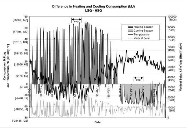
The graph in Figure 9 displays the calculated daily difference in heating or cooling consumption over the one-year period, “exp.” indicates the experiment period. The incident daily vertical solar radiation, and the outdoor temperature is also shown in this figure. The occasions in winter where the LSG windows outperform the HSG windows are all days with very low solar gains. On these days, differences in the thermal performance of the windows come into play.
It is apparent from the consumption graph that, in terms of energy, the benefits from the LSG windows in the summer are outweighed by the resulting increase in consumption in winter. However, when the
same results are converted into cost, assuming 2006 utility prices of $0.52/m3 of natural gas and $0.10/kWh
electricity, the summer savings become more important but still don’t overtake the heating savings. This effect is shown in Figure 10, where the difference in cost due to the LSG windows is plotted on a daily basis. At these prices, the use of HSG in the Test House will cost less than the use of LSG windows.
The total expected heating and cooling consumption and costs using the two glazing technologies are listed in Table 2. Based on this annual analysis, the use of LSG windows in place of HSG windows in the Test House would cost C$26 more, and require an additional 3015 MJ (2,858,000 Btu) of energy.
Difference in Heating and Cooling Consumption (MJ) LSG - HSG -30 -20 -10 0 10 20 30 40 50 60 1-O c t-05 1-N o v-05 1-D e c-05
1-Jan-06 1-Feb-06 1-Mar-06 1-Apr-06 1-May-06 1-Jun-06 1-Jul-06 1-Aug-06 1-Sep-06
Date Consumption, MJ/day and Temperature, °C [B tu/day, °F] 0 10000 20000 30000 40000 50000 60000 70000 80000 90000 100000 Vertical Solar, kJ/m 2/day [Btu/ft 2/day] Heating Season Cooling Season Temperature Vertical Solar [881] [1761] [2642] [3522] [4403] [5283] [6164] [7044] [7925] [8806] [-28435, -22] [-18956, -4] [-9478, 14] [0, 32] [9478, 50] [18956, 68] [28435, 86] [37913, 104] [47391, 122] [56869, 140] exp. exp.
Figure 9. Annual projection of results: Difference in heating and cooling consumption (“exp.” Indicates the experimental period)
Difference in Cost of Heating and Cooling LSG - HSG -1.00 -0.80 -0.60 -0.40 -0.20 0.00 0.20 0.40 0.60 0.80 1.00 01-Oct-05 01-N ov-05 01-D ec-05
01-Jan-06 01-Feb-06 01-Mar-06 01-Apr-06 01-May-06 01-Jun-06 01-Jul-06 01-Aug-06 01-Sep-06
Date Cost ($Cdn/day) 0 10000 20000 30000 40000 50000 60000 70000 80000 90000 100000 Vertical Solar, kJ/m 2/day [Btu/ft 2/day]
Heating Season Cost Cooling Season Cost Vertical Solar [881] [1761] [2642] [3522] [4403] [5283] [6164] [7044] [7925] [8806] exp. exp.
Figure 10. Annual projection of results: Difference in cost of heating and cooling (“exp.” Indicates the experimental period)
Table 2. Total Calculated Annual Consumption and Cost from the use of Glazing Technologies in the Test House (Nov 2005 to Oct 2006)
Analytical Energy Analysis HSG LSG Difference (L-H) Difference, % (L-H)/H Space Heating (21°C) Natural Gas, m3 [ft3] 1171 [41353] 1291 [45591] 120 [4238] 10.3% Electricity, kWh 2225 2251 26 1.2%
Total Heating Energy, MJ [Btu] 51686
[4.8989E+07] 56259 [5.3323E+07] 4573 [4.3344E+06] 8.8% Cost of Heating, C$ 809 874 65* 7.2%* Space Cooling (26°C) Electricity, kWh 2094 1661 -433 -20.7%
Total Cooling Energy, MJ [Btu] 7537
[7.144E+06] 5979 [5.667E+06] -1558 [-1.477E+06] -20.7% Cost of Cooling, C$ 188 149 -39 -20.7%
Annual Energy, MJ [Btu] 59223
[5.6133E+07]
62238 [5.8990E+07]
3015
[2.858E+06] 5.1%
Net Annual Cost, C$ 998 1024 26 2.6%
DISCUSSION
While the analytical projection of experiment results favoured the HSG technology by C$25/year, there are many factors that influence this end result.
In this experiment, the house’s heating demand was met by a high efficiency gas furnace. In terms of energy, the benefits from the HSG windows during winter are nearly 3 times greater than the comparative energy savings from the LSG technology during summer. Despite the season being longer, the peak loads being higher, and the sun being lower in the sky (and thus enabling the windows to have a larger impact) in heating season than in cooling season, the low cost of natural gas compared to the cost of electricity diminishes the overall impact of the HSG windows. Were the same heating provided by an electric furnace, the percent dollar savings would equal the percent energy savings, so the overall financial benefit from the HSG windows would increase.
Similarly, the mode of house operation is very important. During both the heating and cooling seasons, the houses are maintained at a constant setpoint, with continuous circulation and all windows sealed. Different setpoints, or thermostat setting strategies from those used in the experiment would influence savings. For details on how different thermostat setting strategies affect the twin house consumption, please refer to Manning, 2007. Additionally, the experiment does not take advantage of free cooling on cool nights at the beginning and end of the cooling season. A strategy of opening windows at night to let in the cool air would reduce the overall air conditioning loads, and likely reduce the overall cooling savings from the LSG windows. In a house with no air conditioning system, the summer energy savings from the LSG window would not come into play, with the winter performance of the HSG windows. However, the LSG windows did result in cooler air temperatures in south facing rooms than the HSG windows, up to 1.0°C (1.8°F) at mid-height, which may lead to increased occupant comfort during summer.
The orientation of the house and windows also plays a role in the resulting savings from HSG and LSG technology. The twin houses are south-oriented with a large proportion of windows on the south face. This orientation was chosen specifically at the design phase in order to maximize the potential free solar gains in winter. However, the south-orientation also means a high amount of solar gains in summer which must be handled by the air conditioning system. Other orientations would likely have less solar gains – thus, increasing the heating load, and reducing the cooling load. Modeling is required in order to determine the full effect of orientation on energy consumption.
Finally, the difference in SHGC was not the only factor affecting window performance during this
experiment. The LSG windows had a lower average window U-factor (1.62 W/m2°K [0.29 Btu/hr.ft2.°F])
than the HSG windows (1.76 W/m2°K [0.31 Btu/hr.ft2.°F]). Thus, one would expect a better thermal
performance from the LSG windows – particularly during winter, when the indoor to outdoor temperature differential was high. Evidence of this was seen both on winter experiment days with very low solar gains (see Figure 6) – when the LSG windows were able to produce 10 MJ/day (9500 Btu/day) more savings than the HSG windows, and on cold nights – when the interior pane of the LSG window was ~1°C warmer than the HSG pane. Even though the LSG windows prevented more heat losses than the HSG technology, solar heat gains played a larger role. The greater solar heat gains permitted by the HSG windows produced up to 55 MJ (52000 Btu) more savings than the LSG windows on a single sunny winter day, resulting in a substantial advantage in heating season energy performance.
Despite the limitation of these field test results to this particular house, location, year, orientation, and operation, the results are still of great use. The field test results will be used to refine simulation tools. In turn, these models will allow these very limited results to a be projected to variety of operating conditions and climate zones, enabling a broader comparison of the performance of HSG windows to LSG windows. CONCLUSION
In January/February 2006 and July 2006, a side-by-side field assessment of two glazing technologies was performed at the twin R-2000 house facility in Ottawa, Canada. The whole house impact of a high-solar gain glazing technology was compared to a low-high-solar gain glazing technology for a period of 28 days in winter, and 23 days in summer. Measured factors included: incident solar radiation, cooling and heating energy consumption, room temperatures, and window surface temperatures.
Surface temperatures on the inner surface of the LSG windows (surface 4) were up to 12.3°C (22.1°F) cooler in winter, and 7.9°C (14°F) cooler in summer than would be expected for the HSG windows. These
lower temperatures result in less heat radiating into the room, and are thereby one factor that contributes to higher heating loads and lower cooling loads. Room temperatures also provide similar evidence of decreased solar gains due to LSG windows: on sunny winter days, temperatures in south facing room were up to 3.8°C (6.8°F) cooler at mid-height in rooms with LSG windows than HSG windows. In summer, the effect was less pronounced due to the higher position of the sun, the room was up to 1.0°C (1.8°F) cooler at mid-height with the LSG windows.
A pyranometer mounted vertical behind the window indicated that the LSG glazing transmitted 17% less solar radition than the HSG (~57% transmission). This reduction in solar gains due to the use of LSG windows resulted directly in an increase in furnace gas consumption during the heating season, and a decrease in air conditioner electrical consumption during the cooling season. During the winter experiment, the average increase in heating consumption over the duration of the experiment was 23.9 MJ/day (22,700 Btu/day), an increase of 8.7% in gas consuption, and 1.3% in furnace fan electrical consumption. During summer, the average decrease in cooling consumption due to the LSG windows was 14.8 MJ/day (14,000 Btu/day) a 17.7% reduction in cooling electrical consumption.
Correlations between energy consumption and incident vertical solar radiation were developed for both the LSG and HSG windows. These experiment correlations were used to project the experiment data to a full year, to determine the expected annual impact of the different glazing technologies on consumption. For the period of November 2005 to October 2006, the cost of operating the Test House with LSG windows in place of HSG windows is expected to cost C$26 more, and require an additional 3015 MJ (2,858,000 Btu) of energy. Savings from HSG windows would be higher when installed in a house with electrical furnace, or in a home without air conditioning.
Although results from the field test are limited to this particular installation, location, orientation, operating conditions and year, the results were used to refine and benchmark computer simulation tools. In turn, these simulation tools were used to compare the glazing technologies in a number of different situations, to determine the locations where the use of HSG or LSG technology would be most beneficial. Simulation results are planned to be published seperately.
ACKNOWLEDGEMENTS
Thanks are extended to Pilkington North America for providing partical funding for this project, and to Sylvain Harnay and Roger Marchand for their assistance with instrumentation and documentation.
REFERENCES
ASHRAE. 2004. ANSI/ASHRAE Standard 90.2-2004: Energy-Efficient Design of Low-Rise Residential
Buildings. ISSN 1041-2336. Atlanta: American Society of Heating, Refrigerating, and Air-Conditioning Engineers Inc.
ASHRAE. 2005. 2005 ASHRAE Handbook of Fundamentals (SI). 8.12 Atlanta: American Society of Heating, Refrigerating, and Air-Conditioning Engineers Inc.
Barry, C.; Elmahdy, H.; 2007. Selection of Optimum Low-E Coated Glass Type for Residential Glazing in
Heating Dominated Climates. Glass Processing Days. June 2007. Tampere: Finland.
Galasiu, A.D., C.F. Reinhart, M.C. Swinton and M.M. Manning. 2005. Assessment of Energy Performance
of Window Shading Systems at the Canadian Centre for Housing Technology, IRC-RR-196. Ottawa: NRCC.
Gusdorf, J., C. Simpson, M. Swinton, T. Forrest, F. Szadkowski and T.J. Hwang . 2005. Modified Air
Circulation and Ventilation Practice to Achieve Energy Savings and Fuel Switching, NRCC-47712. Ottawa: NRCC.
Gusdorf, J., S. Hayden, E. Entchev, and M. Swinton. 2003. Final Report on the Effects of ECM Furnace
Motors on Electricity and Gas Use: Results from the CCHT Research Facility and Projections,NRCC-38500. Ottawa: NRCC.
Manning, M.M.; Swinton, M.C.; Szadkowski, F.; Gusdorf, J.; Ruest, K. 2007. “The Effects of thermostat setting on seasonal energy consumption at the CCHT Twin House Facility," ASHRAE Transactions, 113, (1), pp. 1-12. Atlanta: American Society of Heating, Refrigerating, and Air-Conditioning Engineers Inc. Parekh, Anil. In Press. “Comparison of Residential Energy Use with High and Low Solar Heat Gain
Swinton, M.C., Manning, M.M.; Elmahdy, A.H.; Parekh, A.; Barry, C.; Szadkowski, F. 2007. "Field assessment of the effect of different spectrally selective low emissivity glass coatings on the energy consumption in residential application in cold climates," 11th Canadian Conference on Building Science and Technology (Banff, Alberta, March 22, 2007), pp. 1-16.
Swinton, M.C., H. Moussa, and R. Marchand. 2001. Commissioning twin houses for assessing the
performance of energy conserving technologies, NRCC-4499. Ottawa: NRCC.
Swinton, M.C., H. Moussa, E. Entchev, F. Szadkowski, and R. Marchand. 2000. Assessment of the Energy Performance of Two Gas Combo Heating Systems at the Canadian Centre for Housing Technology, B-6001. Ottawa: NRCC.