Analysis of nonlinear electroelastic continua with electric conduction

(1)

Analysis of Nonlinear Electroelastic Continua with

Electric Conduction

by

John E. Harper

B.S. Aeronautical Engineering (1995)

Rensselaer Polytechnic Institute

Submitted to the Department of Aeronautics and Astronautics

in partial fulfillment of the requirements for the degree of

Master of Science in Aeronautics and Astronautics

at the

MASSACHUSETTS INSTITUTE OF TECHNOLOGY

June 1999

@

Massachusetts Institute of Technology 1999. All rights reserved.

A

Author

...

_{Department of A....eronau...tics and Astronautics..}

Department of Aeronautics and Astronautics

May 21, 1999

C ertified by ... : ... ...

Nesbitt W. Hagood IV

Associate Professor

Thesis Supervisor

Accepted by...

_..

_\\

Jaime Peraire

Chairman, Department Graduate Committee

(2)

(3)

Analysis of Nonlinear Electroelastic Continua with Electric

Conduction

by

John E. Harper

Submitted to the Department of Aeronautics and Astronautics on May 21, 1999, in partial fulfillment of the

requirements for the degree of

Master of Science in Aeronautics and Astronautics

Abstract

This thesis presents the nonlinear theory for large deformation electroelastic continua with electric conduction. This theory is suitable for modeling actuator and sensor devices composed of deformable, electromechanically coupled, highly insulating ma-terials. Consistency is proven between the large deformation theory and the classical Poynting vector based piezoelectric small deformation theory, extended for electric conduction. A result is that electric body forces, realized mathematically as elec-tric surface tractions, are retained in the small deformation approximation. A finite element formulation is presented suitable for performance analysis of deformable elec-tromechanical actuator and sensor devices composed of highly insulating materials with nonlinear response functions, under the small deformation approximation. Re-sults demonstrate the significant cumulative effects of a weak electric current flow for electric voltage DC offset loading of a highly electrically insulating composite device. Thesis Supervisor: Nesbitt W. Hagood IV

(4)

(5)

Acknowledgments

The work was sponsored by ONR Grant N00014-96-1-0691 with Dr. Wallace Smith serving as technical monitor.

(6)

(7)

List of Figures

2-1 Motion Xt from Bo to t. . . . . . . . . . .. 2-2 Surface of discontinuity for generalized Gauss' theorem. 2-3 Line of discontinuity for generalized Stokes' theorem. . 5-1 5-2 5-3 5-4 5-5 5-6 5-7 5-8 5-9 5-10 . 22 . 50 . 52

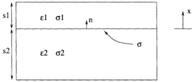
Two layer body geometry: Example 5.2.3. . ... . 100

Active fiber composite: finite element mesh. . ... . 109

Active fiber composite dimensions, in [m] * 10-6 ... 109

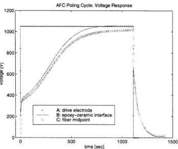
Voltage response through thickness. . ... 110

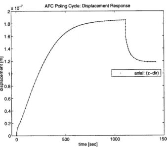
Axial end face displacement. ... . . .. ... . 111

Transverse centerline displacements. . ... . 111

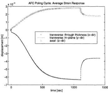
Average axial and transverse strains. . ... . . 112

Fiber centerline strains. ... ... . 112

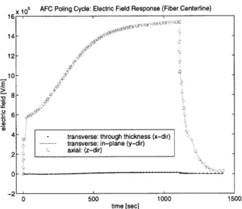
Fiber centerline electric field response. . ... 113

Fiber centerline stress response. ... .. . 113

(12)

(13)

List of Tables

(14)

(15)

Chapter 1 Introduction

1.1 Motivation

Engineering analysis techniques are used in design and development of actuator and sensor devices to predict the performance of a candidate design. Accurate device analysis allows the engineer to optimize a design for a given performance objective and constraints. Alternately, inaccurate device analysis could lead to poor designs and device failure.

This thesis considers analysis of highly electrically insulating deformable bodies subject to electrical and mechanical loading. The response of such highly insulating devices can be influenced or dominated by the cumulative effects of a very weak electric current flow. Much of the engineering analysis literature is concerned with perfect electrically insulating deformable bodies. The perfect insulator approximation is only accurate provided the time scales of loading are sufficiently fast to prevent the cumulative effects of a weak electric current flow. Device designs based on perfect insulator analyses are likely to fail when subjected to sufficiently slow time scale loadings.

1.2 Objective

This thesis will report on the mathematical abstraction of deformable electromechan-ical actuator and sensor devices composed of highly electrelectromechan-ically insulating materials. A first objective is to present a clear exposition with detailed proofs of the nonlin-ear large deformation theory of electroelastic continua with electric conduction. A second objective is to investigate the consistency between this general electroelastic continua theory and the classical small deformation piezoelectric theory based on Poynting vector interpretations, extended for electric conduction. A third objective is to develop an engineering analysis tool for deformable electromechanical actuator and sensor devices composed of highly insulating materials with nonlinear response functions (e.g., repolarizable piezoelectric ceramic material), suitable for arbitrary device geometry and loading conditions.

(16)

1.3 Background

An excellent monograph on the analysis of electroelastic perfect electrically insulating bodies subject to the assumption of small deformations is TIERSTEN's [29] Linear

Piezoelectric Plate Vibrations. TIERSTEN presents the balance of energy equation

for the classical small deformation theory based on the notion of Poynting's vector as the electric energy flux vector across a surface. The result is a local form of the energy expression containing the scalar product of electric field vector with the time derivative of electric displacement vector. The theory presented in TIERSTEN'S monograph can be extended to include the effects of weak electric current density by retaining the electric current density term in Poynting's vector and appending to the system of equations the entropy inequality axiom. As noted by TIERSTEN, the effects of large deformation and electric body forces have been ignored. A natural question to ask is how accurate is this small deformation theory compared to the general large deformation theory, and what are the effects of the ignored electric body forces? This question can be answered by studying the large deformation theory of electroelastic

continua and the consequences of introducing a small deformation approximation. A large deformation theory of electroelastic continua, independent of Poynting vector interpretations, has been developed. See DIXON & ERINGEN [9], MAUGIN &

ERINGEN [17] , ERINGEN & MAUGIN [11] for derivations based on a space (volume) averaging procedure, and TIERSTEN [30], TIERSTEN & TSAI [35], and DE LORENZI

& TIERSTEN [8] for derivations based on a well defined model of interpenetrating continua. A necessary prerequisite would be a study of large deformation continuum

mechanics theory, see ERINGEN [10], OGDEN [21], and GURTIN [15]. We remark that

these two derivations result in equivalent theories, and it is worthwhile to study both approaches. An excellent monograph summarizing this large deformation electro-magnetic theory is ERINGEN & MAUGIN's [11] Electrodynamics of Continua I which contains as a special case the electroelastic theory with electric conduction that we

are interested in.

Solutions of the large deformation equations can be difficult to obtain, and there-fore introduction of a small deformation approximation is frequently carried out in the literature. Examples of small deformation analyses, usually superposed on a large deformation, have been presented, for example, by TIERSTEN [31, 33, 32, 34],

BAUMHAUER & TIERSTEN [3], TIERSTEN & TSAI [35], DE LORENZI & TIER-STEN [8], and also MAUGIN, ET AL [19], ERINGEN & MAUGIN [11], ERINGEN [12], MAUGIN & POUGET [18], ANI & MAUGIN [1].

In all of the above works, the starting point of the analyses are the large defor-mation electroelastic equations. Reduction to the small defordefor-mation equations make explicit exactly what terms are being neglected. Clearly it is desirable to begin an analysis from such a framework. A natural question to ask is, are the equations used in the classical small deformation theory, based on Poynting vector interpretations, consistent with the large deformation theory? The primary equation of concern is the balance of energy expression. Indeed, THURSTON [26] has asked this consistency question regarding the perfectly insulating electromagnetic continua theory. He in-troduces a total energy function as the sum of an internal energy function and a free

(17)

space energy term, then transforms the energy equation in terms of the total energy function to material fields. THURSTON demonstrates that introducing a so-called thermostatic approximation, that ignores certain velocity and magnetization terms, will result in an energy expression that simplifies under the small deformation ap-proximation to the classical energy expression derived using Poynting's vector. Use of the thermostatic approximation is not very satisfactory of a reconciliation between the two theories, and suggests the classical small deformation piezoelectric theory is not consistent with the general electroelastic theory.

THURSTON's result, however, is very interesting. Indeed, the unsatisfactory

ther-mostatic approximation is not needed if the energy equation1 is restricted from elec-tromagnetic continua to electroelastic continua. Although THURSTON does not em-phasize this, the transformed energy expression for electroelastic continua will be exactly consistent, under the small deformation approximation, with the classical energy expression based on Poynting's vector.

MCCARTHY & TIERSTEN [20], working with large deformation semiconducting electroelastic continua, present a transformation for the balance of energy in terms of material fields. The derived balance of energy expression2, under the small deforma-tion approximadeforma-tion and simplified to electric conducdeforma-tion, will be exactly consistent with the classical form of the energy expression relying on Poynting's vector when extended to include electric conduction.

An approach using THURSTON'S transformed energy expression for perfectly in-sulating continua and MCCARTHY & TIERSTEN's transformed energy expression for semiconducting continua can be used to prove consistency between the large mation electroelastic continua with electric conduction and the classical small defor-mation piezoelectric theory relying on Poynting's vector interpretation, extended for electric conduction. Such a study is certainly worthwhile, as it exposes the assump-tions and approximaassump-tions inherent in the classical small deformation theory, including

the role of electric body forces.

TIERSTEN'S monograph Linear Piezoelectric Plate Vibrations is concerned with the analysis of highly electrically insulating piezoelectric bodies in vibration, and therefore does not consider the effects of electric conduction. In fact, highly insulat-ing materials are almost always assumed to be perfectly insulatinsulat-ing. It is important to recall that all highly insulating materials, classified in the engineering literature as electrical insulators, will support non-zero electric conduction currents, usually referred to as leakage currents in elementary physics texts [39, 38, 16]. Under suf-ficiently fast dynamic loading of a highly insulating body, the cumulative effects of weak electric conduction currents are typically negligible, and the perfect insulator approximation may very well be an excellent one.

On the other hand, if the loading time scales are such that very weak electric currents have a cumulative effect, then an analysis based on the perfect insulator approximation could be very inaccurate. Consider the example of a highly insulating piezoelectric device under a sufficiently high frequency sinusoidal electrical loading.

'See eq. 13.48 on p.162 of [26]

2

(18)

In this case, the pefect insulator approximation may be an excellent one. However, consider the same device under identical high frequency electrical loading, but with an additional electric voltage DC offset. After a sufficiently long period of time the cumulative effects of the weak electric current flow will dominate the voltage offset response. This is an example of a typical loading condition on highly insulating devices when electric conduction will in general be signifcant.

1.4 Thesis Contributions

This thesis is based on the recognition that highly electrically insulating actuator and sensor devices under general electrical and mechanical loading must be analysed in the framework of electroelastic continua with electric conduction. This thesis presents

a detailed account of the nonlinear theory for large deformation highly insulating electroelastic continua with electric conduction, and proves the consistency between this theory and the classical small deformation piezoelectric theory based on Poynting vector interpretations, extended for electric conduction. The essential step is proving the equivalence of the balance of energy equations in the two theories. A consequence is that electric body forces, recognized mathematically as electric surface tractions, are naturally retained in the small deformation approximation. Finally, this thesis presents a finite element formulation suitable for performance analysis of deformable electromechanical actuator and sensor devices composed of highly insulating materials with nonlinear response functions (e.g., repolarizable piezoelectric ceramic material) and arbitrary device geometries, under the small deformation approximation.

1.5 Thesis Outline

Our presentation is in the framework of continuum physics. We introduce the notion of a body as a collection of points. Deformation is a mapping of the body from some reference configuration to a new deformed configuration. The notion of change of observer and change of reference configuration is introduced. These will be needed for deducing restrictions on the constitutive functions, as required by our constitu-tive theory axioms. Mathematical results essential to the development are presented. Fundamental axioms of the continuum physics theory are presented in terms of spatial fields. Differential equations are derived from the integral form statements. Jump conditions are derived from integral form statements extended to include surfaces of discontinuity. Constitutive equations are derived in terms of an internal energy function and a total energy function. We introduce the notion of material fields, and systematically derive equivalent material field representations of the global and local equations. Constitutive equations are derived from the material fields, which automatically satisfy the material objectivity axiom. Jump conditions in material fields are derived from integral form statements extended to surfaces of discontini-nuity. These are needed to piece together solutions across material discontinuities, and specialize to boundary conditions on the bounding surface of a body. The small

(19)

deformation approximation is introduced to simplify the governing equations. A weak form of the resulting small deformation equations is presented as a starting point for our finite element formulation. Solution techniques for the finite element equations are presented, with results from analysis of a piezoelectric fiber embedded in an epoxy matrix under an electric voltage DC offset loading, using a nonlinear material model for repolarization.

(20)

(21)

Chapter 2 Large Deformation Electroelastic

Equations

2.1 Introduction

This chapter presents essential theorems and proofs in the nonlinear large deformation theory of electroelastic continua with electric conduction. The differential equations and jump conditions needed for device analysis are summarized in chapter 3 for convenience.

2.2 Bodies, Deformations, and Motions

1 Bodies have the property that they occupy regions of three dimensional Euclidean point space S. An arbitrary point x in E is associated with a position vector x in three dimensional Euclidean vector space E, relative to an arbitrarily choosen origin point o E S. For fixed o, x and x have a unique correspondence, and we can identify

the point x with the vector x. When o is fixed in 5, we use x to denote both a point in 9 and its corresponding position vector in E.

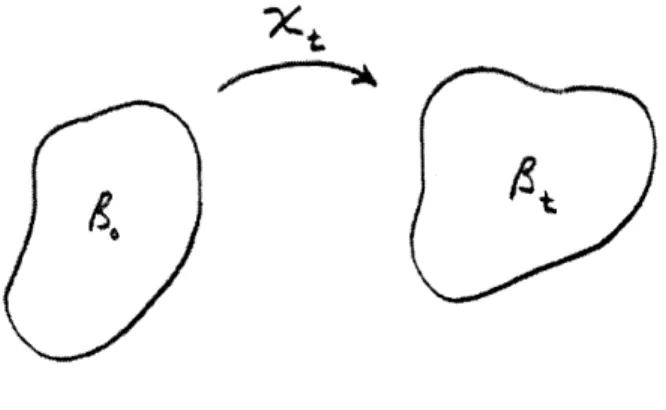
We define a body B as a regular region' in S. In general, B will occupy different regions of 9 at different times2 t E IR. For convenience we choose one such region B3o

as the reference configuration of B. Points in the body can be identified with their positions in B. We call points X E B3o material points. A deformation X carries the body from its reference configuration B3o to a deformed configuration Bd and carries each material point X to a point x,

y:X

~x, 1_{This section is based on}_OGDEN _{[21, pp. 77-83]}

'A closed region is the closure of a connected, open set in 9. A regular region is a closed region

with piecewise smooth boundary.

2

(22)

where we write,

Bd =

3

₀

).

The motion Xt of B is a smooth one-parameter family of deformations parameterized

xt

Figure 2-1: Motion Xt from 3o to Bt.

by time t. The region Bt is called the current configuration of B, and the point x is called the spatial point occupied by the material point X at time t,

Xt : X-+x.

We write

B,= X (o

, t),

x = x(X,t).

Axiom 2.2.1 (Axiom of Continuity) 2 Throughout the body B the motion Xt and

its inverse are single-valued and as many times continuously differentiable as required.

The inverse mapping Xt 1 _{takes the deformed body B3t back to its reference}

configu-ration 3o. We write

Bo = X (Bt, t),

X = x-1 (0,t).

If we choose our reference time corresponding to Bo, at t = 0, then the reference configuration Bo necessarily satisfies

Bo = (Bo, 0),

Bo = X-1 (Bo, 0).

2

(23)

2.3 Observer Transformations

3 Suppose an event in the physical world manifests itself at a point of Euclidean point space 8 and at a time in IR. This event will be recorded by an observer O as occuring at (x, t). If x and xo are distinct points of 8 and t and to are distinct times in IR, then two events observed by O at (xo, to) and (x, t) are seperated by a distance lax - xoll

in 8 and a time interval t - to in IR. The definition of an observer transformation

is based on the notion that different observers must agree about distance and time intervals between events.

Definition 2.3.1 (Change of Observer) An observer transformation or change of

observer is defined as any transformation that takes (xo, to) and (x, t) to (x, to) and

(x*, t*), such that distances and time intervals are preserved, 4

t-to = t*-t*.

The general form of such a transformation is,

X* = Q (t) + b (t), t* = t - a

Q'Q

=

QQ'= I

det(Q) = +1,

where a is an arbitrary scalar, b(t) is an arbitrary vector, and Q(t) is an arbitrary orthogonal tensor. It is convenient to restrict Q(t) to arbitrary proper orthogonal

tensors, such that det (Q) = 1.

Remark 2.3.2 (Observer Transformation) For the motion Xt of a body B, an

observer transformation or change in observer X is,

x*(Xt*) =

Q(t)

(X,t) + b(t) t* = t - a. (2.1)

Q'Q = QQ'=I

det (Q) = 1.

A transformation (2.1) that takes (x, t) to (x*, t*) is interpreted as a change of ob-server from O to O*, such that the event recorded by O at (x, t) is the same event as that recorded by O* at (x*, t*). In general, the description of a physical quantity associated with the motion Xt of a body B depends on the choice of observer. Such a distinction will be important for deducing restrictions on constitutive equations for material response.

3_{This section is based on OGDEN [21, pp. 73-77] and GURTIN [15, pp. 139-145]} 4_The_2-norm_is_defined_by, _lxill₌₍₌

(24)

2.4 Fields, Deformations, and Integral Theorems

5 To introduce definitions of material and spatial fields, we define the reference set T and the trajectory set T as

T = ((X,t) X E Bo, t

IR

1 ,R

T = (x, t)I x B, tE IR}.

Definition 2.4.1 (Material and Spatial Fields) A material field is a function

with domain T7-. A spatial field is a function with domain T.

Remark 2.4.2 (Fields) All fields defined over T are assumed to be as many times

continuously differentiable as required. Surfaces and lines of discontinuity will be addressed in section 2.14.

Much of the theory presented involves integrals over volumes, surfaces, and lines contained in either Bo or Bt. Here we introduce notation to distinguish between sets of points in the two configurations.

Definition 2.4.3 (Volumes, Surfaces, and Lines in 3o and 3)

* A material volume Vo is a volume in B3o. The material volume V is the volume in Bt occupied by the material points X E Vo at time t,

v=x(Vo, t) .

* A material surface So is a surface in Bo. The material surface S is the surface in Bt occupied by the material points X

E

So at time t,

S = (S, t) .

* A material line Co is a line in 3o. The material line C is the line in Bt occupied by the material points X E Co at time t,

c=X(Co, t)

Many of the proofs will be made more transparent by introducing a Cartesian coor-dinate system and manipulating vectors and tensors in their component form.

Definition 2.4.4 (Cartesian Coordinate System) Material and spatial fields will

be referred to a single Cartesian coordinate system fixed in S. The set of basis vectors for this system will be denoted by either ik or iK, with indices k, K = 1, 2, 3.

(25)

Definition 2.4.5 (Summation Convention) Summation over once repeated

in-dices is understood.

For example,

XMiM = Xlil + X 2i2 + X 3i3.

A material point located in the reference configuration Bo by P and in the current configuration B3t by p are represented in the Cartesian coordinate system by

P = XMiM, p = Xkik.

Definition 2.4.6 (Component Notation Convention) Components associated with

the reference configuration Bo will consistently have capital indices. Components as-sociated with the current configuration Bt will consistently have lower case indices.

Frequently both spatial and material fields will be presented and manipulated in their component form. For example, a spatial vector field A, a material tensor field B, and a two-point tensor field F are referred to the Cartesian coordinate system by'

A = Akik,

B = BRs iR 0 is,

F FkR ik iR. (2.2)

Consistent with our convention, the fields A, B, and F can be written in component form as Ak, BRS, and FkR respectively. Similarly, the motion Xt of a body may be written in component form as

Xk Xk (XM, t), (2.3)

XM = xTM (xk, t) . (2.4)

We will occasionally abuse notation by not distinguishing between the function and its value in (2.3) and (2.4). For example,

Oxk k _{(_}(XJ, t)

OXM OXM

XM _ 1Ox (X, t)

&Xk Xk

Integral transformations will be needed to rewrite conservation laws originally defined over Bt, in terms of fields over Bo. For example, if boundary conditions are only known in terms of the reference configuration B13, then it can be useful to rewrite the governing equations in terms of fields over Bo.

'The tensor product (or dyadic product) of two vectors a and b is denoted a®b and has Cartesian components (a 0 b)i_j = aibj

(26)

Definition 2.4.7 (Jacobian Determinant) The Jacobian determinant J is assumed

to be strictly positive for all time t,

J = det (X )> 0.

Theorem 2.4.8 (Transformations of Arc, Area, and Volume) A material

el-ement of arc dxi in the current configuration Bt is related to its elel-ement of arc dXj in the reference configuration 13o by

8xi

dxi = x dXj. (2.5)

ax,

A material element of area ni dS in Bt is related to its element of area Nj dSo in Bo3 by

oXJ

ni dS = J Nj dSo. (2.6)

axi

A material element of volume dV in Bt is related to its element of volume dV in B13 by

dV = J dVo. (2.7)

Proof. See ERINGEN [10, pp. 45-48] or OGDEN [21, pp. 83-89] for a proof. 0

Definition 2.4.9 (Kronecker Delta) The Kronecker delta symbol, 5_{ij, is defined}

by

i6j

i= 0 i#j

Consider a material vector field AK and a spatial tensor field Bij. It can be verified directly from definition 2.4.9 that the Kronecker delta symbol has the property of

changing indices,

AK 6KM = AM,

Bij 6

jk " Bik.

Definition 2.4.10 (Alternating Symbol) The alternating symbol, Eijk, is defined by

1 if (ijk) is a cyclic permutation of (123)

Eijk = -1 if (ijk) is an anti-cyclic permutation of (123)

0 otherwise

Consider two spatial vector fields a and b. It can be verified directly from definition 2.4.10 that the vector cross product of two vectors and the alternating symbol are

(27)

related by,

(a x b) = Ei_jkajbk. (2.8)

A direct consequence of (2.8) is an expression for the curl of a vector field in terms of the alternating symbol,

(V X b)i =

Eijkbk,j-Useful expressions for the determinant and cofactor of a 3 x 3 matrix Aij in terms of the alternating symbol are"

1

det (Aij) = EijkepqrAipAjqAkr,

1

cofactor (Aip) = -EijkEpqrAjqAkr. (2.9)

Recall, the cofactor matrix and determinant satisfy'

det (Aij) (Aij)- 1 = cofactor (Aji) . (2.10) Consider a material tensor field TJK. It can be verified directly from definition 2.4.10 that the equation

EIJKTJK = 0

implies that the anti-symmetric components of TJK are identically zero, T[JK] = 0.

Using (2.3) and (2.4) for fixed time t we obtain

dZk = Xk dXM, (2.11)

&XM OXM

dXM = dxk. (2.12)

From the chain-rule of differention, we obtain the useful relations

OXk OXM 6

OXM OX

XM 6

MN. OXzk (XN

6_See_SEGEL_{[23, pp. 14-23] for discussion on the alternating symbol and determinants} 7

(28)

We will frequently introduce a symmetric/anti-symmetric decomposition in our proofs and statements. To simplify our presentation we introduce the following notation. Definition 2.4.11 (S/A Decomposition) The symmetric/anti-symmetric (S/A)

decomposition of a tensor Aij is defined as

A(ij= (Aij + Aji)

A =1 (Aid - Aji)

Aij = A(ij) + A[ij].

The deformation and strain tensors introduced next will appear when transforming our equations from spatial to material fields. They also appear when material response functions depending on the displacement gradient are required to be invariant under

observer transformations.

Definition 2.4.12 (Deformation and Strain Tensors) The deformation tensor CMN and the strain tensor EMN are defined as

OZk Oxk

CMN(XL, t) - Xk Xk

aXM XN'

1

Zxk Oxk

EMN(XL, t) - (aM XN MN )

The significance of these tensors is illustrated below. Consider elements dP in Bo

and dp in Bt,

dP = dXMiM,

dp = dxkik. The square of these elements are

dS2 = dXMdXM, ds2 dxk dxk &Xk Oxk X XdXM dXN, OXM aXN CMNdXdX NdX.

The measure of change of length for the same material points in Bo and Bt is

ds2 - dS2 ( Xk XkN -6MN dXM dXN,

- 2_{EMN dXM}_dXNy.

(29)

partial differentiation with respect to a coordinate. For example, aXk Xk, M - _X XM' XM,1, =OXM XM, k --OXk

In continuum physics theory, the time rate of change following a material point Xk is frequently encountered. We therefore introduce the following notation.

Definition 2.4.14 (Material Time Derivative) The material time derivative

op-erator is defined as the time rate of change following a material particle XM,

d a

dt a XM

Definition 2.4.15 (Material Velocity) The material velocity field Vk is defined as

ak (Xj, t)

Vk- t XM

Proposition 2.4.16 (Material Time Derivative: Spatial Fields) The material

time derivative of any spatial field / (Xk, t) is

d- - + vk , k. (2.13)

dt at

Proof. Introducing Xk = Xk (XK, t) and using the chain rule

=# = + __ __

dt _at _aXk _{at XM}

= +vk ,k.

at

In continuum mechanics it is natural to express balance laws in terms of integrals over material lines, material surfaces, and material volumes in Bt. Below we state some results that will be useful in working with such integrals.

Lemma 2.4.17 The material time derivative of the Jacobian determinant J is

J = Jvk,k (2.14)

Proof. From (2.9) we write

1

(30)

Differentiating J with respect to Xr,R and using (2.9) and (2.10), OJ 1 Xr, -ErjkCRJKXj, JXk, K -ax, R 2 = _{cofactor (r, R)} JXR,r.

Taking the material time derivative of J

OJ d

J ((,R) = JXR,rVr,R

OXr, R dt

proves (2.14). a

Lemma 2.4.18 The material time derivative of the deformation gradient XJ,k is

d

dt (XJ, i) = -XJ,k Vk, i (2.15

Proof. Take the material time derivative of

XJ,k Xk,K "- JK,

and multiply the result by XK,i to obtain d

=(X,i)

= -XJ,kvk,n n,KXK,i

- -XJ,k k,n ni. (2.16)

Equation (2.16) proves (2.15). 0

Below we derive three useful theorems for material time derivatives of integrals over material lines, material surfaces, and material volumes in Bt.

Remark 2.4.19 (Integrals over Elements of Bo) According to definition 2.4.14,

the material time derivative operates holding material points X E Bo constant, there-fore, the material time derivative operator commutes with integrals defined over

ele-ments in o,.

Theorem 2.4.20 (Material Time Derivative: Line Integral) The material time

derivative of a line integral of any spatial field q over a material line C in Bt is

dt

f

dxi = _{(0 dxi- + vi, j dxj).} _(2.17)

Proof. Transform the integral over elements in Bt to an integral over elements in

(31)

Co, and transform the integral back into an integral over elements in Bt, d d f dxi dt c d =

_{dt c'}

x 2,;jdX = i,±

+

vi,) dXj

= 6ij + Ovi, j) dx.

Equation (2.18) proves (2.17).

Theorem 2.4.21 (Material Time

time derivative of a surface integral in Bt is

Derivative: Surface Integral) The material

of any spatial field 0 over a material surface S

dt

fs

n dS = [( + CVk,k) ni - bVk, ink] dS. (2.19) Proof. Transform the integral over elements in Bt to an integral over elements in B3o using (2.6), commute the material time derivative operator with the integral over So, use the relations (2.14) and (2.15), and transform the integral back into an integral over elements in Bt,

d-

d _{JXj, iNj dSo}

dt _so

= o [JXj,i + OJXj,i + Jd (X,i)] N dSo

= f [JX i + CJvk,kXJ, - CJXJ,kk,i] NJ dSo SJ + vk,k)

XJ,i

- vk,iXJk] 1xr, J nr

dS

=

j

+ v)k, k ir - vk, i 6kr]

nr dS.

o (2.20) Equation (2.20) proves (2.19).

Theorem 2.4.22 (Material Time Derivative: Volume Integral) The material

time derivative of a volume integral of any spatial field q over a material volume V in Bt is dV = dV. dt v dV (2.21) (2.22)

S+

(k),k dV

Proof. Transform the integral over elements in Bt to an integral over elements in Bo using (2.7), commute the material time derivative operator with the integral over Vo,

(2.18)

d Cni dS

d Oni dS

(32)

use the relation (2.14), and transform the integral back into an integral over elements in Bt, d f OdV d + JV = 4JJdVo

dt

v

dt vo

= ( J + J) dVo J (0 + k, k

J

dVo = + vkk) dV. (2.23)

Equation (2.23) proves (2.21). Using (2.13) in (2.21) proves (2.22). E

2.5 Fundamental Axioms of Electromagnetics and

Thermomechanics

8 This section presents the fundamental axioms of electromagnetics and thermome-chanics for deformable continua, including both fluids and solids. The electromagnetic equations are presented in terms of rationalized MKS units'. The axioms of electro-magnetism are defined over spatially fixed line, surface, and volume integrals. In our presentation below, we take these integrals to coincide at time t with the deformed body Bt.

Definition 2.5.1 (Fields)

co = permittivity of free space Po = permeability of free space

E = electric field vector in 3t H = magnetic field vector in Bt

P = polarization vector in Bt

D = electric displacement vector in B3t

D = E + P,

M = magnetization vector in Bt

B = magnetic induction vector in Bt H = -B-M,

Po

qF free charge per unit volume in 3t J' = electric conduction current in 3

t (with respect to fixed frame) J = total electric current in Bt (with respect to fixed frame)

8

This section is based on ERINGEN & MAUGIN [11, pp. 72-81] 9_{See ERINGEN & MAUGIN [11, p.}_406]

(33)

J = J'+ qFv

p = mass per unit volume in Bt, Po = mass per unit volume in Bo,

fE = electromagnetic or electric force per unit volume in Bt, fi = non-electromagnetic force per unit mass,

ti = force per unit area in Bt,

ti = 7jinj,

ji = Cauchy stress tensor,

CE = electromagnetic or electric body couple per unit volume in Bt, = internal energy per unit mass,

E = electromagnetic or electric power per unit volume in Bt,

h = heat power per unit mass, q = heat flux per unit area in 8t,

77 = entropy per unit mass,

E

= absolute temperature.

Axiom 2.5.2 (Gauss' Law)

D.ndS = fqFdV. (2.24)

Axiom 2.5.3 (Conservation of Magnetic Flux)

sB.ndS = 0. (2.25)

Axiom 2.5.4 (Faraday's Law)

SE.dx = fB n dS. (2.26)

Axiom 2.5.5 (Ampere's Law)

H .dx = J -ndS + - DndS. (2.27)

Axiom 2.5.6 (Conservation of Mass) The total mass of a material body B is

un-changed during the motion Xt of the body.

p dV =

Jpo

dV (2.28)

Axiom 2.5.7 (Balance of Momentum) The time rate of change of momentum of

the material body is equal to the resultant force acting upon the body.

(34)

Axiom 2.5.8 (Balance of Moment of Momentum) The time rate of moment of

momentum of the material body is equal to the resultant moment of all forces and the resultant of all couples acting on the body.

d

xxpvdV

=

xx(pf

+

fE)

+

E]dV

+

xxt

ds.

(2.30)

or in component form,

SEknjXnvj

dV=

f

[knjxn Pf E) + CkE

dV

+

j

eknntj

dS.

(2.31)

Axiom 2.5.9 (Conservation of Energy) The time rate of change of the sum of

the internal and kinetic energies of a material body, considered as a closed system, is equal to the sum of the rate of work of all forces and couples and the energies that enter or leave the body per unit time.

d

v

iv+ p) dV = (E + ph + pfivi) dV

+

f

(tivi - qini) dS. (2.32)

Axiom 2.5.10 (Law of Entropy) The time rate of the total entropy is never less

than the sum of the entropy supply due to body sources and the entropy influx through the surface of the body.

d dV d - _{ni dS .} _(2.33)

Axiom 2.5.11 (Postulate of Localization) The axioms hold true for any volume

element in V, any surface element in S, and any line element in C.

2.6 Maxwell's Equations

This section deduces the local balance laws from the global axioms.

Theorem 2.6.1 (Maxwell's Equations) The local equations (2.34)-(2.37) are

equiv-alent to (2.24)-(2.27), V D = qF, (2.34) V -B = 0, (2.35) OB Vx E = t (2.36)

at

OD Vx H = J + (2.37)

Proof. Commute the partial time derivative with the spatially fixed integrals (coinciding at time t with Bt). Applying (A.1), (A.2) to (2.24)-(2.27), and invoking the postulate of localization proves (2.34)-(2.37). 0

(35)

Proposition 2.6.2 (Conservation of Charge) The conservation of charge

equa-tion,

V - J + = 0, (2.38)

is a consequence of Maxwell's equations (2.34) and (2.37).

Proof. Take the partial time derivative of (2.34) and the divergence of (2.37),

o

OqF OD _QqF

S(V - D)= Oq V. - (2.39)

at

Ot

-t

t'

V. J+- )=V.(Vx H) V J+-

a

=0. (2.40)

Equation (2.38) follows from (2.39) and (2.40).

Definition 2.6.3 (Electromagnetic Energy of Free Space) The electromagnetic

energy of free space UF is defined as

UF =- I(oE.E+ B.B). (2.41)

2 PO

Theorem 2.6.4 (Poynting's Theorem) All fields satisfying Maxwell's equations

(2.34)-(2.37) satisfy the identities

OD aB E - J + E - + H = -V (Ex H), (2.42) _P

aB

aU

F E -J + E M + = -V (E x H). (2.43)

at

Proof. Take scalar product of (2.37) with E, and using the vector identity

V-(E x H)= H-(V x E)- E. (V x H),

obtain

OD

E - J = H - (Vx E)- V - (Ex H)- E (2.44)

Using (2.36) in (2.44) proves (2.42). Using (2.41) in (2.42) proves (2.43).

Remark 2.6.5 (Poynting's Vector) The vector (E x H) in (2.42) and (2.43) is

called Poynting's vector and its surface integral is interpreted as the surface flux of electromagnetic energy. In integral form, Poynting's theorem appears mathematically as a conservation statement, with Poynting's vector as a surface flux term,

OD aB

E-J+E

t-

+H -

)

dV

=-

(ExH)-ndS.

(36)

Physical arguments in support of the Poynting vector interpretation can be found in

STRATTON [25].

2.7 EQS Maxwell Equations

In this section the electroquasistatic (EQS) Maxwell equations are defined. These equations are Maxwell's equations (2.34)-(2.37) with the magnetic induction term

assumed negligible, see HAUS & MELCHER [16], and TIERSTEN [27]. The EQS

equations are a good approximation for materials with small electric current flow, where magnetic fields are presumed negligible.

Definition 2.7.1 (EQS Field) The EQS electric displacement D is defined as

D = coE + P. (2.45)

Definition 2.7.2 (Negligible Magnetic Induction) The magnetic induction and

its partial time derivative are assumed negligibly small,

OB _{~ 0,}

(2.46)

at

B 0. (2.47)

Remark 2.7.3 (Approximations) Equation (2.46) is the usual EQS

approxima-tion, permitting a non-zero static magnetic induction field. Equation (2.47) is an additional approximation used to eliminate magnetic terms from the electromagnetic body force and body couple equations (2.73) and (2.80).

The EQS Maxwell equations are,

V - D = qF, (2.48)

V B = 0, (2.49)

VxE = 0, (2.50)

OD

Vx H = J+ (2.51)

The magnetic field term H can be eliminated by taking the divergence of (2.51) and the partial time derivative of (2.48) to form the conservation of charge statement (2.38). If H is desired it can always be determined from (2.51) once D and E are known. From this point on the EQS Maxwell equations will be defined by:

Definition 2.7.4 (EQS Maxwell Equations)

V D = qF, (2.52)

Vx E = 0 - E = -V, (2.53)

aqF

V. J+ = 0. (2.54)

(37)

Definition 2.7.5 (EQS Poynting Vector) The EQS Poynting vector (E x H)EQS is understood as notation for a vector and is defined by

(E x H)EQS = (2.55)

Definition 2.7.6 (Electric Energy of Free Space) The electric energy of free space

UF is defined

UF = -oE E. (2.56)

2

under the EQS approximation.

Theorem 2.7.7 (EQS Poynting's Theorem) All fields satisfying the EQS Maxwell

equations (2.52)-(2.54) satisfy the identities OD

E J + E = - V . (E x H)EQs, (2.57)

OP OUF

E J + E + = -V . (E x H)EQS. (2.58)

at

Proof. Using (2.53) and the vector identity

V x (H) = V x H + V x H,

gives

-V.(ExH) = V.[Vx (¢H)]-V. (Vx H),

= -V (¢V x H). (2.59)

Using (2.37), (2.59), (2.55), and (2.46) in (2.42) proves (2.57). Using (2.45) and (2.56)

in (2.57) proves (2.58). E

We will find it convenient to work with a reduced form of the EQS Maxwell equations that do not contain free charge qF explicitly. First we note the integral form of the EQS equations.

Proposition 2.7.8 (EQS Maxwell: Integral Form) The integral form of the EQS

Maxwell equations (2.52)-(2.54) are

sDni dS = fVqFdV (2.60)

cE dxi = 0 (2.61)

dfq'dV

+/ JJndS = , J, = Ji - qFvi (2.62) Proof. Integrating (2.52) over a material volume V in spatial coordinates and using (A.1) proves (2.60). Integrating (2.53) over an open material surface S in spatial

(38)

coordinates and using (A.2) proves (2.61). Integrate (2.54) over a material volume V in spatial coordinates and use (A.1) to obtain

JnidS + qdV = 0. (2.63)

Using (2.22) and (A.1) in (2.63) proves (2.62). a Proposition 2.7.9 (Reduced EQS Maxwell: Integral Form) The EQS Maxwell

equations (2.60)-(2.62) are equivalent to

d Dini dS +f Jni dS -0 (2.64)

c Ei dxi= 0 (2.65)

Proof. Taking the material time derivative of (2.60) and using in (2.62) proves

(2.64). U

It will be useful to define the following convective time derivative.

Definition 2.7.10 (Convective Time Derivative) The convective time derivative

of a spatial vector field Di is defined as

D* = Di + Divk,k - Dkvi,k (2.66)

This definition is motivated by (2.19) and satisfies

d Dini dS = D ni dS. (2.67)

Proposition 2.7.11 (Reduced EQS Maxwell: Local Form) The local form of

the reduced EQS Maxwell equations (2.64) and (2.65) are

(D* + J), = 0 (2.68)

(Vx E)i = 0 -+ E = -,i (2.69) Proof. Equation (2.67) in (2.64) and postulate of localization proves (2.68). Equa-tion (A.2) in (2.65) and postulate of localizaEqua-tion proves (2.69). •

2.8 Conservation of Mass

This section derives the local form of conservation of mass, and also presents a useful material derivative relation.

Theorem 2.8.1 (Local Conservation of Mass) Local conservation of mass

equiv-alent to (2.28) is

(39)

Proof. Taking the material time derivative of (2.28), using (2.22)

(p + PVk, k) dV = 0, (2.71)

and taking (2.71) for arbitrary volumes V (postulate of localization) proves (2.70). * Proposition 2.8.2 (Material Derivative Relation) Any spatial field q satisfies

the following identity for integrals over a material volume V d

- fpBdV =f pbdV. (2.72)

Proof. Consider an aribtrary function q. Using (2.21) and conservation of mass (2.70) we obtain the useful relation

df PodV =

d

d pdV v (p ) + (p)vk, k dV,

fp= p + ( + pvk, k) dV,

= fp dV.

2.9 Balance of Momentum

Expressions for electromagnetic body force density fiE acting on deformable continua

have been derived in DIXON & ERINGEN [9], MAUGIN & ERINGEN [17], ERINGEN & MAUGIN [11] based on volume (space) averaging techniques, and in DE LORENZI

& TIERSTEN [8] based on a well-defined interpenetrating continua model. The DE

LORENZI & TIERSTEN paper is a generalization of earlier works by TIERSTEN [30]

and TIERSTEN & TSAI [35].

Definition 2.9.1 (Electromagnetic Body Force) A polarizable, magnetizable, and

electrically conducting deformable media will experience an electromagnetic body force per unit volume in B3t (to a first approximation) of the form10

fE = qFEi + PjEi,j + EijkvjPnBk,n + PijkjBk + MB,i + EijkJjBk. (2.73)

P

Introducing approximation (2.47) eliminates magnetic force density terms from (2.73) resulting in the electric body force density definition.

10

See DE LORENZI & TIERSTEN [8, eq. 3.44, p. 944]. Equation (2.73) is equivalent to ERINGEN & MAUGIN [11, eq. 3.5.26, p. 59]

(40)

Definition 2.9.2 (Electrical Body Force) A polarizable and electrically

conduct-ing deformable media will experience an electric body force per unit volume in Bt (to a first approximation) of the form

fqE = Ei + PjEi,j. (2.74)

Proposition 2.9.3 (Electrical Stress Tensor) The electrical body force density fE

defined by (2.74) can be written as the divergence of a second order tensor TE

fiE= , (2.75)

E _{PjE, +}

eoEE - 1-oEkEk6ji,

= DjEi - UFji. (2.76)

Proof. Taking divergence of (2.76) and using (2.52), (2.45), and (2.56)

1

TE _(DjEi),j

-2E (EkEk6ji),j , Dj, jE + D Ei,j - eoEjEj, i, = qFE, + PjEij

Theorem 2.9.4 (Local Balance of Momentum) Local balance of momentum

state-ments equivalent to (2.29) are

(Ti +T), + P (fi - ii) 0, (2.77)

7ji,j + fiE ₊_P_(fi_- _i) ₌_0. _(2.78)

Proof. From (2.72)

df pvi dV = pvi dV.

and noting

S[i(nj)

+ tE(nj)] dS (ji j + T ) _{nj dS,}

= (i +

),

1 dV. our balance of momentum statement becomes

S ji

+ ) , + fi - pJi] dV. (2.79)

Taking (2.79) for arbitrary volumes V (postulate of localization) proves (2.77). Using equation (2.74) in (2.77) proves (2.78). N

(41)

2.10 Balance of Moment of Momentum

An expression for the electromagnetic body couple density CE in deformable con-tinua is derived in ERINGEN & MAUGIN [11] based on a volume (space) averaging techniques.

Definition 2.10.1 (Electromagnetic Body Couple) A polarizable, magnetizable,

and electrically conducting deformable media will experience an electrical body couple per unit volume in Bt (to a first approximation) of the form11

CE = PxE+MxB+vx(PxB). (2.80)

Introducing approximation (2.47) eliminates magnetic couple terms from (2.80) re-sulting in the electrical body couple definition:

Definition 2.10.2 (Electrical Body Couple) A polarizable and electrically

con-ducting deformable media will experience an electrical body couple per unit volume in Bt (to a first approximation) of the form

CE = eijkPjEk, (2.81)

CE = P x E.

Theorem 2.10.3 (Local Balance of Moment of Momemtum) Local balance of

moment of momentum equivalent to (2.31) is

T[nj] = E[,P]. (2.82) Proof. Noting SknjXnTijni dS =

/

(eknjXnTji),i dV = ECkj (x,Tj + X-nTji) dV, = Fknj (6niij + XnTij,i) dV, f vknj (7nj + xT-ij, i) dV. (2.83) Using (2.21) _ f knjxnpvj dV = - (eknjxnpvj) + knjxnPvjvk,k dV , = E, kn, (vnpvj + xnvj + XnPij + xnpvjvk,k) dV. (2.84) "

(42)

Using (2.83) and (2.84), (2.31) becomes

V kni [v (p + PVk, k) - xn = JV kdV.

Using (2.70) and (2.78), (2.85) becomes

f (EknjTn + C) dV =0

Recalling (2.81), (2.86) becomes

(-pij +pfj fjE Tij,i)

-- EknjTn + CkO.

eknj (n]j + PnEj) = 0

[njl = -PinEj].

Using the anti-symmetric relationship

-PInE] = E[nPj]. in (2.87) proves (2.82).

Definition 2.10.4 (Partial and Total Stress Tensors)

tensors TiP and TT are defined as

7j = i + j ,

= ji + DjEi - UF6ij.

The partial and total stress

(2.88) (2.89) (2.90)

The stress tensors TjP and TjT defined above appear in our presentation of the consti-tutive equations.

Proposition 2.10.5 (Symmetry of Partial and Total Tensors)

rT are symmetric S= ₀ T Tji - 0 Tensors Tj and (2.91) (2.92) Proof. Recalling the fact

E[jPi] = -P[jEi]

and using (2.82) we obtain the anti-symmetric part of Tji as

T[ji] = -P[jE]. (2.93) - Tnj] dV (2.85) (2.86) T7nj] + P[nEj] = 0, (2.87) 0

(43)

Introducing the S/A decomposition of

T

and using (2.93)

P P P

- Ti) + T[jil

T(ji)

+

T[ji] + P(jE)

+

P[jEi]

= T(ji) + P(jE,) (2.94)

Equation (2.94) proves (2.91). Similarly decomposing rjT and using (2.93)

T T

Tj T7i) + Vii]

= T(ji) + T[ji] + P(jEi) + PEi] + EoEE - UF6ij

- T(ji) + P(jE) + coEjE - UFSij (2.95)

Equation (2.95) proves (2.92).

2.11 Electromagnetic Power

12 Expressions for the electromagnetic power density _E_{for deformable continua have} been derived in DIXON & ERINGEN [9], MAUGIN & ERINGEN [17], ERINGEN &

MAUGIN [11] based on volume (space) averaging technqiues, and in DE LORENZI & TIERSTEN [8] based on a well-defined interpenetrating continua model. The DE

LORENZI & TIERSTEN paper is a generalization of earlier works by TIERSTEN [30]

and TIERSTEN & TSAI [35].

Definition 2.11.1 (Electromagnetic Power Density) A polarizable, magnetizable,

and electrically conducting deformable media has electromagnetic power per unit vol-ume in Bt (to a first approximation) of the form13.

OBi (2.96)

E= (PE,i + qfEj) vj + EipHi + JiEi - 11 (2.96)

Pi

J = Ji qF i (2.97)

M = M + (vx P)i.

Proposition 2.11.2 (Equivalent Electromagnetic Power) Electromagnetic power

density E is equivalent to

OP OBi

E = E t- M + JiEi + (E Pivj),j. (2.98)

12This section is based on THURSTON [26, pp. 157-163] 1 3_See_{DE LORENZI}_&

TIERSTEN [8, eq. 4.4, p.944]. Equation 2.96 is equivalent to ERINGEN & MAUGIN [11, eq. 3.5.41, p. 61]

(44)

Proof.

n=i

=d = p-p, dt

(p

-2p

Using (2.70) -i = P-li ₊ _P-2ipvj, j,

plIi

= Pi + PiVk,k, api at + vkPi,k + Piv, k.

Recalling the Maxwell equation (2.36),

-

M' at= -M

_--

_a

+ (v x P)j(V x E)i.

Noting the vector identity,

(v x P)i(V x E)i = VkEi,kPi - PkEi, kVi,

- M t

=

- A

M

-- + vkEi, kPi - PkEi, k i,

-t OP

E = E

-

+ EPiv,j + JiJ - Mj

n-a

at O

+ vjEi,jPi + Evj Pi,j.

Grouping terms to obtain (EiPivj),j in (2.101) proves (2.98).

2.12 Conservation of Energy:

tinua

Electroelastic

Con-In this section we establish a series of equivalent statements for conservation of energy. Theorem 2.12.1 (Conservation of Energy I) Conservation of energy for elec-troelastic continua is

+ pE) dV Sfv (E + ph + pfivi) dV

+ S(tjvj - qini) dS,

= pEfIi + _{(PEj,i +} _qFEj)_vj

J- = Ji - qF i, (2.102) + JEi, (2.103) (2.104) (2.105) (2.99) (2.100) we obtain (2.101) pvivi

Analysis of nonlinear electroelastic continua with electric conduction

Analysis of Nonlinear Electroelastic Continua with

Electric Conduction

by

John E. Harper

B.S. Aeronautical Engineering (1995)

Rensselaer Polytechnic Institute

Submitted to the Department of Aeronautics and Astronautics

in partial fulfillment of the requirements for the degree of

Master of Science in Aeronautics and Astronautics

at the

MASSACHUSETTS INSTITUTE OF TECHNOLOGY

June 1999

@

Massachusetts Institute of Technology 1999. All rights reserved.

Author

...

Department of A....eronau...tics and Astronautics..

Department of Aeronautics and Astronautics

May 21, 1999

C ertified by ... : ... ...

Nesbitt W. Hagood IV

Associate Professor

Thesis Supervisor

Accepted by...

..

\\

Jaime Peraire

Chairman, Department Graduate Committee

Analysis of Nonlinear Electroelastic Continua with Electric

Conduction

by

John E. Harper

Abstract

Acknowledgments

Contents

List of Figures

List of Tables

Chapter 1

Introduction

1.1

Motivation

1.2

Objective

1.3

Background

1.4

Thesis Contributions

1.5

Thesis Outline

Chapter 2

Large Deformation Electroelastic

Equations

2.1

Introduction

2.2

Bodies, Deformations, and Motions

y:X

3

).

xt

B,= X (o

, t),

2.3

Observer Transformations

Q'Q

QQ'= I

Q(t)

2.4

Fields, Deformations, and Integral Theorems

T = ((X,t) X E Bo, t

IR

1 ,R

E

8xi

ax,

oXJ

1

at

f

_{Department of A....eronau...tics and Astronautics..}

_..

_\\

_{dt c'}