Designing and Assessing the Architectural Speech Security of Meeting Rooms and Offices

(1)

Publisher’s version / Version de l'éditeur:

Vous avez des questions? Nous pouvons vous aider. Pour communiquer directement avec un auteur, consultez la

première page de la revue dans laquelle son article a été publié afin de trouver ses coordonnées. Si vous n’arrivez

Questions? Contact the NRC Publications Archive team at

PublicationsArchive-ArchivesPublications@nrc-cnrc.gc.ca. If you wish to email the authors directly, please see the first page of the publication for their contact information.

https://publications-cnrc.canada.ca/fra/droits

L’accès à ce site Web et l’utilisation de son contenu sont assujettis aux conditions présentées dans le site

LISEZ CES CONDITIONS ATTENTIVEMENT AVANT D’UTILISER CE SITE WEB.

Research Report (National Research Council of Canada. Institute for Research in Construction), 2006-08-01

READ THESE TERMS AND CONDITIONS CAREFULLY BEFORE USING THIS WEBSITE.

https://nrc-publications.canada.ca/eng/copyright

NRC Publications Archive Record / Notice des Archives des publications du CNRC :

https://nrc-publications.canada.ca/eng/view/object/?id=d42fa469-f76b-4ff7-9d69-16b8bef22b24 https://publications-cnrc.canada.ca/fra/voir/objet/?id=d42fa469-f76b-4ff7-9d69-16b8bef22b24

NRC Publications Archive

Archives des publications du CNRC

For the publisher’s version, please access the DOI link below./ Pour consulter la version de l’éditeur, utilisez le lien DOI ci-dessous.

https://doi.org/10.4224/20377425

Access and use of this website and the material on it are subject to the Terms and Conditions set forth at

Designing and Assessing the Architectural Speech Security of Meeting Rooms and Offices

(2)

http://irc.nrc-cnrc.gc.ca

Designing and Assessing the Architectural Speech Security of

Meeting Rooms and Offices

I R C - R R - 1 8 7

B r a d l e y , J . S . ; G o v e r , B . N .

(3)

Acknowledgements

This report brings together the results of several projects that have been funded by Public Works and Government Services Canada (PWGSC), the Royal Canadian Mounted Police (RCMP) and the National Research Council (NRC). The details of the previous projects are described in various reports that are listed in the references section of this report.

(4)

Summary

This report brings together several research studies to explain how to design meeting rooms to be speech secure and how to measure the degree of speech security of existing rooms. Speech security refers to a high level of speech privacy and corresponds to conditions in which it is difficult to understand speech from an adjacent room. For a high degree of speech privacy, transmitted speech might be barely intelligible or not even audible to an

eavesdropper. Architectural speech security indicates that it is the speech security provided by the building construction and building systems.

The new Speech Privacy Index, SPI, was developed from extensive listening tests to rate the intelligibility and audibility of speech sounds from an adjacent room. This measure is a uniform weighted signal-to-noise level difference over the speech frequencies from 160 Hz to 5 kHz. It is calculated from 1/3 octave band speech and noise levels at the position of the listener and quantifies the thresholds of intelligibility and audibility as well as the

intelligibility of transmitted speech.

A new procedure to measure the speech security of a meeting room is described that is based on measuring the level difference of a test sound between room-average sound levels in the meeting room and the levels of the transmitted sound at spot-receiver positions close to the outside of the meeting room.

The measured level differences are used to determine the transmitted speech levels at the spot-receiver positions. The transmitted speech levels and the ambient noise levels at the spot-receiver positions outside the room are used to calculate SPI values. The acceptability of conditions can be determined by comparing the resulting SPI values with those for the threshold of intelligibility of speech or the threshold of audibility of speech.

Because speech levels in meeting rooms and ambient noise levels outside meeting rooms vary from moment to moment, the probability of the transmitted speech being intelligible or audible to an eavesdropper is related to the probability of various combinations of speech and noise levels occurring. New statistical information on the likelihood of various speech and noise levels occurring can be used to predict the probability of speech being intelligible or audible to an eavesdropper.

In this report the step-by-step details of the new measurement procedure are described. It is also explained how the same approach can be used at the design stage, including several examples. An Appendix includes a representative selection of sound transmission data for walls, windows and doors that can be used for initial design studies.

(5)

1. Introduction

The more general term speech privacy is used to describe a wide range of conditions where there is some degree of difficulty in understanding speech. Speech privacy can vary from the often marginal speech privacy in some open-plan offices, to the near-perfect privacy that is possible for enclosed rooms. Enclosed meeting rooms and offices are said to be speech secure when it is very difficult for an eavesdropper outside the room to understand speech from inside the room. That is, speech security refers to situations where there is a high degree of speech privacy. Architectural speech security is intended to limit discussion to the effects of the building and building systems on speech privacy.

We can measure speech privacy in terms of the intelligibility of speech, that is, the percentage of words that can be understood. When a very low percentage of speech is intelligible, we have conditions with relatively high speech privacy. However, in some cases even zero intelligibility is not good enough, and we can strive to attain conditions where speech is not even audible outside the room.

Whether speech from an adjacent meeting room is intelligible or even audible depends on three factors: (a) the sound isolation characteristics of meeting room boundaries, (b) the levels of speech sounds in the meeting room, and (c) the levels of ambient noise at listener positions outside the meeting room. When the transmitted speech sounds are loud enough relative to the ambient noise at some listener position, the speech will be audible and sometimes also intelligible. We can measure the sound isolation characteristics of meeting rooms or design new rooms to meet desired characteristics. However, speech levels in meeting rooms and noise levels outside meeting rooms vary from moment to moment and should be considered as statistical quantities with probabilities of various speech and noise levels occurring. Therefore we can define speech security as a condition where transmitted speech is likely to be either intelligible or audible for no more than some specific very small percentage of the time. For very high degrees of speech security, the transmitted speech would extremely rarely be either intelligible or audible.

This report explains a new procedure for designing and measuring the architectural speech security of meeting rooms. Chapter 2 first describes the basic principles on which the new method is based. This includes new information on the probabilities of occurrence of various speech levels in meeting rooms and various ambient noise levels outside the meeting rooms. Chapter 2 also explains the basic concept of the measurement procedure for assessing the sound isolating characteristics of the room boundaries, including the calculation of the new Speech Privacy Index (SPI). The subsequent chapters describe the steps required to either assess the speech security of an existing room, or to design a new speech secure meeting room.

(7)

2. Basic Principles

To consider the speech privacy of a meeting room, one first measures or predicts the sound transmission characteristics of the boundaries of the room. Then one of two approaches can be taken to decide if the condition will correspond to adequate speech privacy. The first approach is to use a specific combination of speech level in the meeting room and ambient noise level at the listener’s position as design values for calculating the Speech Privacy Index, SPI. The relation of this value to the SPI for the threshold of intelligibility or to the threshold of audibility would indicate the degree of speech privacy for that combination of speech and noise level. The other approach is to use the measured transmission

characteristics of the room boundaries to estimate the probability of speech from the meeting room being intelligible or audible at listening positions outside the room.

While the Speech Privacy Index involves physical measurements, interpreting the

measurements requires an understanding of how often the transmitted speech will be audible or intelligible to a human listener located outside of the meeting room. To respond to this need, section (a) below explains how the SPI measure is related to the results of extensive listening tests. Section (b) describes the calculations required to obtain SPI values. Finally, section (c) explains how the statistical properties of speech levels in meeting rooms and ambient noise levels outside the meeting rooms can be used to interpret the SPI values in terms of the likelihood of a speech privacy lapse occurring (i.e. the transmitted speech being audible or intelligible).

(a) What Can People Hear or Understand?

The intelligibility of speech is primarily related to the level of the speech relative to the level of concurrent ambient noise. That is, the louder the speech is relative to the ambient noise and any other competing sounds, then the more intelligible it will be. Therefore we can estimate intelligibility from signal-to-noise ratios that measure the level of the speech relative to the level of the noise. Since speech privacy corresponds to low speech intelligibility, we also measure speech privacy in terms of signal-to-noise ratio measures.

A number of signal-to-noise ratio measures have been used in the past. The difference between the A-weighted speech and noise levels is perhaps the simplest measure, but is not so well related to actual speech intelligibility scores. The Articulation Index, AI, and its more recent replacement the Speech Intelligibility Index, SII, are quite sophisticated signal-to-noise type measures that are well related to most speech intelligibility scores. However, we have shown [1,2] that they are not as accurate for the very low intelligibility scores found when evaluating conditions of high speech privacy. This is because both of these measures are limited to values between 0 and 1 and a zero value for these measures does not

correspond exactly to zero intelligibility. AI and SII are also unable to correctly rate the audibility for conditions of speech intelligibility below zero because this would usually require AI and SII values to be less than 0 where these measures are not defined.

Extensive listening tests were used to relate speech intelligibility scores to signal-to-noise type measures and to determine the thresholds of intelligibility and audibility [1,2]. In these tests, subjects listened to combinations of speech and noise simulating listening to speech transmitted through various walls. In one test the percentage of the words of each sentence that were intelligible was used as the speech intelligibility score and related to various

(8)

signal-to noise type measures. In another type of test, the fraction of listeners who were able signal-to hear or understand any speech sounds was recorded. These were used to establish: (i) the

threshold of audibility of speech sounds, (ii) the threshold of audibility of the cadence or rhythm of speech sounds, and (iii) the threshold of intelligibility of speech sounds (i.e. when at least one word is understood). The point at which 50% of the subjects could just hear or just understand the speech was termed the just noticeable threshold.

From these tests the measure that was best related to both intelligibility and audibility judgments was a uniformly weighted signal-to-noise ratio that is called here the Speech Privacy Index and is given by the un-weighted sum of the 1/3 octave band signal-to-noise level differences as follows,

dB f L f L SPI f n ts( ) ( )]/16, [ 5000 160

∑

= − = (2.1)

where in each 1/3 octave band with centre frequency f,

Lts(f) is the transmitted speech level at the listener position, and

Ln(f) is the ambient noise level at the same listener position.

The quantity in the square brackets should be clipped so that it cannot have values less than –32 dB.

If the signal-to-noise ratio in a particular band is less than –32 dB, it is well below the threshold of audibility and such extremely low values would inappropriately exaggerate the degree of speech privacy. Therefore, it is necessary to clip or limit the signal-to-noise level difference values in each 1/3 octave band to be no lower than –32 dB.

-30 -25 -20 -15 -10 -5 0 0 20 40 60 80 100 S p e e c h in te llig ib ili ty, % SPI, dB

Figure 1. Mean intelligibility score versus the SPI.

Figure 1 plots the mean trend of intelligibility scores versus values of the SPI measure obtained from our listening tests. Figure 2 plots the fraction of the listeners who were able to (a) hear some speech sounds, (b) hear the cadence of the speech sounds, and (c) to

(9)

-30 -25 -20 -15 -10 -5 0 0.0 0.2 0.4 0.6 0.8 1.0 Threshold of Intelligibility Cadence Audibiity F ra c ti on a bove thres hol d SPI, dB

Figure 2. Fraction of listeners able to (a) hear some speech sounds (Audibility), (b) hear the cadence of the speech sounds (Cadence), or (c) understand at least one word (Intelligibility). The horizontal

line indicates the 50% points corresponding to the threshold values.

The thresholds of audibility, cadence and intelligibility were defined as when 50% of the listeners could just hear or understand speech. The SPI values corresponding to these thresholds taken from Figure 2 are given in Table 1.

Threshold SPI

Intelligibility -16 dB

Cadence -20 dB

Audibility -22 dB

Table 1. SPI values for the just noticeable thresholds of audibility, cadence and intelligibility.

Thus, if conditions at the listener’s position correspond to SPI = -16 dB, you would expect speech to be barely intelligible to good listeners. Of course, how often this might occur is determined by how likely to occur the speech and noise levels used in the calculations are to occur. That is, we must also consider the likelihood of various speech and noise levels occurring in and near meeting rooms to determine how often speech privacy will be a problem.

(10)

(b) The New Measurement Procedure

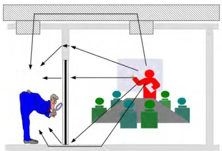
In general, it is necessary to evaluate the possibility of transmitted speech being audible or intelligible at points on all sides of the meeting room and possibly above and below it too. As illustrated in Figure 3, there are many possible sound paths from the meeting room to

adjacent spaces. While the sound isolation characteristics of many walls may be quite homogeneous, there are also often leaks and weak spots such as those near doors.

Figure 3. Illustration of possible sound paths for speech from a meeting room to a nearby eavesdropper.

Conventional sound transmission measurements are based on the difference in room-average measurements of the levels of a test signal such as white noise in both the source and

receiving room. These conventional measurements are intended to provide information on the average sound transmission characteristics of the wall separating the two rooms and do not identify the characteristics of particular leaks and weak spots. They are based on

assumptions of diffuse sound fields that are only approximately correct for rooms that are of regular shape, moderate size and without too much sound absorbing material.

The new method was developed to avoid the limitations of the conventional approach and to provide results that relate directly to our ability to hear or understand transmitted speech in spaces adjacent to meeting rooms. As in the conventional approach, a loud white noise test sound is radiated into the source room. However, the sound transmitted into adjacent spaces is measured at spot-receiver positions usually located 0.25 m from the outside boundaries of the meeting room.

These spot-receiver positions are used for three reasons. First, they more realistically represent more sensitive listening positions where an eavesdropper might logically be located. Second, by measuring a number of such positions one can locate leaks and weak spots in the sound transmission characteristics and not just measure the average

characteristics. Consequently, they are more helpful in identifying the cause and magnitude of any problems that may exist. Third, transmitted sound levels measured at these positions, located relatively close to the room boundary, are much less influenced by the acoustical characteristics of the receiving space. That is, the new approach is not based on any

(11)

assumption of a diffuse sound field in the receiving space. At the same time, the 0.25 m distance from the nearby surface that is radiating the transmitted sound, is large enough to avoid significant level changes due to small errors in the distance of the microphone from the room boundary. Since the space adjacent to a meeting room could be anything from a broom closet to a large open-plan office, it is important to be able to make accurate measurements of the transmitted sounds without the unknown effects of the acoustical properties of the

receiving space.

In the source room (i.e. the meeting room) the white noise test signal is measured for a number of combinations of source and microphone position to get a good room average sound level. The transmission characteristics to adjacent spaces are determined from the level differences between the source-room average levels and the transmitted sound levels

measured at each spot-receiver position. By measuring a source-room average, the

measurements are representative of the possibility of a talker being located any part of the meeting room that is included in the test positions. The same source-room average levels can be used for measurements of the sound transmission from the meeting room to all adjacent spaces. There is no need to repeat the source room measurements for transmission through the different walls of the room. The number of measurements required to get an adequately precise source room average level is greatly reduced by using a sound source that is

approximately omni-directional.

The measured level differences between the source room average level and spot-receiver position levels can be used to calculate the Speech Privacy Index by rearranging equation (2.1) as follows, dB , 16 / )] ( ) ( ) ( [ 5000 160

∑

= − − = f n s f LD f L f L SPI (2.2)

Because, Lts(f) = Ls(f) - LD(f), and in each 1/3 octave band with centre frequency f:

Ls(f) is the source-room average speech level,

LD(f) is the level difference from sound transmission measurements

between the source-room average and the spot-receiver position, and

Ln(f) is the ambient noise level at the spot-receiver position.

The quantity in the square brackets should be clipped so that it cannot have values less than –32 dB.

Because the value in the square brackets is usually not less than –32 dB, equation (2.2) can usually be re-written more simply as,

dB ), avg ( ) avg ( ) avg ( _n s LD L L SPI = − − (2.3)

where: Ls(avg), LD(avg) and Ln(avg) are the arithmetic averages of the 1/3 octave band

values from 160 to 5k Hz.

One can use equation (2.3) to calculate the SPI from measurements of LD(avg) and some design speech and noise levels.

Alternatively one can design to meet a specific SPI value. It is reasonable to design for

SPI = -16 dB, which corresponds to the threshold of the intelligibility of speech. One can

(12)

dB , 16 ) avg ( ) avg ( ) avg ( −L =LD − L_s _n (2.4)

This shows that for a particular SPI value, the average measured level difference, LD(avg), is related to the difference between the source-room speech level and the ambient noise level at the spot-receiver position. That is, it is the difference between the source-room speech level and the spot-receiver ambient noise level that determines whether there will be adequate privacy, not the separate speech and noise levels.

However, the speech and noise levels are statistical in nature, and occasionally much higher speech levels or much lower noise levels may occur. The probability of various combinations of source-room speech level and spot-receiver ambient noise level occurring determines the probability of transmitted speech being intelligible for a given LD(avg) value.

A step-by-step description of the new procedure for measuring transmission characteristics from meeting rooms to adjacent spaces is given in Chapter 3 of this report. The procedure is used to determine level differences over a range of frequencies between source-room average levels and spot-receiver levels. While the spot-receiver positions will most often be located 0.25 m from the room boundary in the adjacent spaces, they will sometimes be located at other positions where potential speech privacy problems are to be evaluated.

(13)

(c) Probabilities of Various Speech and Noise Levels Occurring

For a given meeting room, the probability of speech being heard or understood in an adjacent space is related to the probability of particular speech levels occurring in the meeting room and to the probability of various ambient noise levels occurring in the adjacent spaces. A meeting room with better sound isolation from adjacent spaces will exceed some level of speech privacy more often because the higher speech levels and quieter ambient noise levels required for transmitted speech to be heard or understood, will occur much less often. Therefore, to be able to estimate the probability of a speech privacy problem, we need to know something about the probability of the occurrence of various speech levels in meeting rooms and of various ambient noise levels in spaces adjacent to meeting rooms, in addition to the measured LD(avg) value.

To determine the probability of various speech levels occurring in meeting rooms, sound level loggers were left in a number of meeting rooms described in Table 2 [3]. They were typically located around the periphery of the meeting room just over one metre from the boundaries of the room. These locations were intended to be more representative of speech levels incident on the room boundaries. During each meeting, sound levels were logged in terms of 10 s Leq values. In total over 100,000 of these 10 s Leq values were acquired and they give a good description of the distribution of speech levels in meeting rooms.

Although some rooms included sound amplification systems, speech in rooms with amplification was on average only 2 dBA higher in level than in rooms without

amplification. This is because the speech levels were measured close to the room boundaries at positions more representative of the farthest listeners from the talker. In the larger rooms where amplification was used, the systems were usually adjusted so that speech levels at larger distances were similar to those in smaller rooms without sound systems. Because the effect of amplification was small, all of the data from all meetings were grouped together to determine the probabilities of various speech levels occurring.

Number of meeting room cases* measured

32

Number of meetings measured 79

Number of people in each meeting 2 to 300 people

Range of room volumes 39 to 16,000 m3

Range of room floor areas 15 to 570 m2

Table 2. Summary of meeting rooms measured. ( * includes 30 different rooms, 2 of which were measured with and without sound amplification systems).

Figure 4 shows the cumulative probability distribution of the measured speech levels. This shows the probability of the measured speech level having values up to the speech level given by the horizontal-axis. For example, 90% of the time the speech level was 64 dBA or less. Conversely, 10% of the time the speech level exceeded 64 dBA. The dotted lines on Figure 4 illustrate this example.

(14)

30 40 50 60 70 80 0 20 40 60 80 100 C u mu lat ive pr ob ab ility, % Level, dBA

Figure 4. Cumulative probability distribution of measured speech levels in meeting rooms. (Dotted lines illustrate example in the text).

Similarly, a large survey of ambient noise levels in spaces adjacent to meeting rooms was also carried out [3]. Ambient noise levels were recorded in terms of 10 s Leq values over complete 24 hour periods. Because the ambient noise levels vary systematically with the time of day, these results were broken down into 4 time-of-day periods. The cumulative

probability distributions of the measured ambient noise levels in each of these time periods are shown in Figure 5.

Noise levels tend to be highest during the daytime and lowest at night. For predicting the probabilities of speech privacy problems, the early evening ambient noise levels are used. During this time period noise levels are a little lower and hence privacy problems are a little more likely, but this is a time period when there are likely to be a reasonable number of meetings taking place. Figure 5 shows (see dotted lines) that during the early evening, ambient noise levels in adjacent spaces were less than 33.5 dBA for about 10% of the time.

20 30 40 50 60 0 20 40 60 80 100 C umulat ive p roba bility, % Level, dBA Time of day Daytime Early evening Late evening Night time

Figure 5. Cumulative probability distribution of measured noise levels in spaces adjacent to meeting rooms for daytime (8:00-17:00), early evening (17:00-21:00), late evening (21:00-24:00) and night

(15)

In the examples above, the meeting room speech level was greater than 64 dBA for 10% of the time and the ambient noise levels in adjacent spaces were less than 33.5 dBA for 10% of the time. Since the speech and noise levels are from separate spaces, it is reasonable to assume that the distributions of source room speech levels and spot-receiver ambient noise levels are independent. In this case the probability of both a speech level exceeding 64 dBA and an ambient noise level less than 33.5 dBA is the product of their separate probabilities, or 1%.

If the room were designed to be speech secure for this combination of source room speech level and spot-receiver ambient noise level, then there would only be the likelihood of a speech privacy lapse for 1% of the time that the room is in use. Since there are 2880 of the 10 s intervals in an 8 hour working day, this would correspond to speech privacy being a potential problem for about 29 of those 2880 intervals. This could be reasonably good speech security in that there is rarely the likelihood of a speech privacy problem and the room could be said to be speech secure for 99% of the time. However, for more secure situations the sound isolation of the meeting room would have to be improved so that speech privacy problems would occur even less often.

Because speech and noise levels vary from moment to moment, the actual speech privacy will similarly vary over time. However, we say the room is speech secure if transmitted speech is either intelligible or audible for an adequately small percentage of the time that the room is in use. Consequently a higher degree of speech security would correspond to

transmitted speech being either intelligible or audible less often.

In the above example, the probability of a speech level being higher than the particular value of 64 dBA was the same as the probability of the noise level being lower than the value of 33.5 dBA. It is reasonable to base designs on such equal probabilities of either the source room speech level or the spot-receiver ambient noise level contributing to a lack of speech privacy. Other combinations of equally probable source-room speech and spot-receiver ambient noise levels can be determined by aligning the distributions from Figures 4 and 5 according to their separate probabilities of occurring. This has been done in Figure 6 for pairs of speech and noise levels in terms of their separate probabilities of occurrence.

Equation (2.4) shows that for a given LD(avg) from transmission measurements and a

particular required SPI value, a specific difference between the source room speech level and the spot receiver ambient noise levels is implied. That is, it is the difference in these speech and noise levels and not the separate levels that is important for determining the level of speech privacy. The probability of various (source-room speech level) – (spot-receiver noise level) differences occurring, i.e. Ls(avg)-Ln(avg), determines the probability of the particular

(16)

0.1 1 10 100 20 30 40 50 60 70 80 Level , dBA

Individual probabilities of occurrence, % Speech

Noise

Figure 6. Room average speech levels versus the probability of this level being exceeded (solid line) and spot-receiver (early-evening) ambient noise levels versus the probability of the noise level being

lower than this (dashed line).

The information from Figure 6 can be displayed more usefully by plotting the differences between each pair of equally probable speech and noise levels versus the combined probability of this pair occurring. This is shown in Figure 7. In producing Figure 7, the speech levels and noise levels were converted from A-weighted levels to arithmetic averages over the 1/3 octave bands from 160 to 5k Hz. To do this the speech spectrum was assumed to have a spectrum shape obtained from the average of Pearsons’ male and female raised voice spectra [4], which would be typical of voice levels used in meeting rooms. This average speech spectrum shape is shown in Table 3 with the overall A-weighted levels and the arithmetic average level over the speech frequencies from 160 to 5k Hz. It is seen that the speech frequency average level is 12 dB less than the A-weighted level for this spectrum shape.

Noise levels in spaces adjacent to meeting rooms were found to generally approximate a -5 dB per octave spectrum shape [3], which is often referred to as a ‘neutral’ or Hoth spectrum shape [5,6]. A neutral ambient noise spectrum shape is also included in Table 3. For this spectrum shape the average level over the speech frequency range is 11 dB less than the corresponding A-weighted level.

(17)

0 10 20 30 40 50 60 1E-4 1E-3 0.01 0.1 1 10 100 Com bine d p roba bility of oc curr en ce, %

(Source-room speech level) - (spot-receiver ambient noise level), dB(avg)

Figure 7. Combined probability of occurrence of various differences between source-room speech levels and ambient noise levels at spot-receiver positions outside the room.

(Dotted lines illustrate example in the text).

Frequency, Hz Speech level, dB Noise level, dB

125 46.8 55.0 160 44.3 53.3 200 49.0 51.7 250 53.0 50.0 315 51.3 48.3 400 54.4 46.7 500 56.7 45.0 630 54.7 43.3 800 51.6 41.7 1000 50.1 40.0 1250 51.1 38.3 1600 49.1 36.7 2000 44.6 35.0 2500 43.9 33.3 3150 43.5 31.7 4000 42.6 30.0 5000 39.1 28.3 6300 38.7 26.7 8000 38.6 25.0 dBA 60.7 51.8 dB(avg) 48.7 40.8

Table 3. Speech spectrum from Pearsons’ male and female raised voice level data [4] and -5 dB/octave ‘neutral’ ambient noise spectrum.

(18)

From Figure 7 we can see that if we were to design for a (source-room speech level) - (spot-receiver ambient noise level) difference of 30 dBA, we would expect this to occur about 1% of the time. (Dotted lines on Figure 7 illustrate this eample). However, if we designed for a difference of 40 dBA, Figure 7 indicates that this would occur only about 0.05% of the time and the design would be speech secure for 99.95% of the time. Thus, Figure 7 provides the basic information for determining the probability of a room with a particular LD(avg) value meeting some criterion for speech privacy.

Figure 7 can be further modified to relate the combined probabilities of pairs of meeting room speech levels and spot-receiver ambient noise levels to the related LD(avg) -16 values using equation (2.4). This makes it possible to relate the probability of speech privacy problems directly to measured LD(avg) values. This is included as Figure 9 in Chapter 3 of this report.

(19)

3. Measuring the Architectural Speech Security of a

Meeting Room

(a) Overview

The new procedure measures the reduction from source-room average levels to spot-receiver levels at points usually located 0.25 m from the outside of the source room. This receiver position was selected because it: (a) minimizes the effects of the acoustical properties of the receiving space, (b) it represents a more sensitive listening position for a potential

eavesdropper, and (c) it provides specific point-to-point information about leaks and weak spots in a room boundary. Where transmission may not be a simple direct path through the wall, other spot-receiver positions can also be selected. A source-room average is used to represent the possibility of a talker being almost anywhere in the meeting room. This same source-room average is convenient because it can be used as the source-room level for assessing transmission through all of the boundaries of the room without the need to repeat for each element. The details of the procedure are based on extensive sound transmission measurements from meeting rooms [7].

(b) The Measurement Procedure

Sound Source

A white noise test signal is radiated from one or more loudspeakers into the source room (the meeting room being tested). Each loudspeaker source must approximate an omni-directional sound source. To be an acceptable approximation to an omni-directional sound source, it must meet the omni-directionality requirements included in the ISO 3382 standard. (See Table 4). Meeting these requirements is normally achievable with a dodecahedron loudspeaker.

Frequency, Hz 125 250 500 1000 2000 4000

Maximum deviation, dB ± 1 ± 1 ± 1 ± 3 ± 5 ± 6

Table 4: Maximum allowed directional deviations of the source in decibels for excitation with octave bands of pink noise as measured in a free field.

Source Signal

The input signal to the amplifiers should be random noise containing an approximately uniform and continuous distribution of energy over frequency for each 1/3 octave test band. A white noise electronic source can satisfy this condition and is appropriate for sound transmission measurements.

Frequency Range

The frequency range for measurements must include the one-third octave bands from 160 to 5000 Hz and is referred to as the speech frequency range in this document.

Bandwidth and Filtering

The overall frequency response of the measurement system, including the filter or filters in the source and microphone sections, shall conform to the specifications in ANSI S1.11 for each one-third octave test band, for Order 3 or higher and Type 1 or better filters.

(20)

Measuring Equipment

Microphones, amplifiers, and electronic circuitry to process microphone signals and perform measurements must satisfy the requirements of ANSI S1.4 for Type 1 sound level meters, (but without the requirement for B and C weighting networks).

Measurement quality microphones, 13 mm or smaller in diameter, and that are close to omni-directional below 5000 Hz shall be used.

While it is possible to measure in each 1/3-octave band sequentially, this is not very

practical. A sound level analyser that measures levels in all bands simultaneously is strongly preferred.

Measurement of Average SPL in the Source Room

At least two source positions shall be selected in the central part of the source room. These positions must be well separated and at least 2 m apart and at least 1 m from any large reflecting surfaces such as the room boundaries. The source shall be 1.5 m above the floor in the source room. If the meeting room is both larger than 200 m3 and is estimated to have a mid-frequency reverberation time less than 0.5 s, then a minimum of 4 source positions should be used. For these rooms, larger spatial standard deviations of measured sound levels are expected. Using a larger number of source positions will increase the precision of the source-room average and the resulting SPI value.

For each source position in the source room, the average sound pressure level, SPL, in the source room, and the SPL at each spot-receiver position must be measured. If two sources are used simultaneously, separate statistically independent noise generators and power amplifiers must be used to drive them.

Meeting Room Adjacent Space

omni-directional source 1.5 m microphone sweep 0.25 m 1.2 - 2.0 m

Figure 8. Speech privacy measurement setup

Levels in the source room must be measured at 4 or more independent locations or alternatively by using a walking microphone sweep. If four independent microphone positions are to be used they should be well-separated and at least 1 m apart and away from significant reflecting surfaces.

(21)

To make a walking sweep measurement, the source room average level is determined from an Leq measurement in 1/3 octave bands obtained while walking around the room. The operator walks slowly moving the microphone in a circular path of at least 0.5 m diameter in front of him to evenly sample as much as practical of the measurement space. The sound level meter or microphone is held well away from the operator's body - at least 0.5 m (a microphone boom serves to increase the distance). The microphone speed shall remain as constant as practical. The operator shall take care to ensure that the path does not

significantly sample any part of the room volume for more time than other parts.

For either approach, the microphone shall always be more than 1.5 m from the sound source and more than 1 m from the walls of the source room. The integration time shall be at least 30 seconds. This measurement shall be repeated for each source position.

Selection of Spot-Receiver Positions in Adjacent Spaces

Measurements should be made at all locations in the receiving area where possible speech privacy problems are suspected. The regions near doors, windows and other types of weak elements in the boundaries of the room are obvious locations that should be included. Mostly, measurements should be made at positions 0.25 m from the outside boundaries of the source room.

Locations where sound leaks may occur are most efficiently found by initial listening tests. Position the sound source near the middle of the source room and radiate a signal so that the average sound pressure level in the room is at least 80 dBA. With all doors closed, listen carefully at positions outside all boundaries of the source room and identify the locations of probable sound leaks where measurements should be made to assess the speech privacy. In some cases spot measurement locations may not be adjacent to the room boundary. Where there is sound transmission from the room via some flanking sound path such as through ducts, spot measurements should be made at locations where a speech privacy problem is suspected and where a potential eavesdropper might be located.

In addition to the locations identified as probable weak spots, select other positions around the source room so as to provide complete and uniform coverage of the periphery. Most receiving positions will be 0.25 m from the outer surfaces of the room. Other spot-receiver positions may be selected close to suspected weak spots such as ventilation duct openings and doors.

Microphones shall not be closer than 0.25 m from the nearest surface of the source room and must be between 1.2 and 2 m above the floor.

Measurements of SPL shall be made at each receiving position for a period of at least 15 seconds.

The number of spot-receiver position will depend on the complexity of the geometry of the room boundaries and the number of locations where sound leaks are suspected. Some spot-receiver locations should be at positions 0.25 m from the outside boundaries of the room and where no sound leaks are suspected. Where the results at other locations are different to measurement results at these ‘good’ positions some form of relative sound insulation deficiency may be identified.

(22)

Measurements at the Receiving Positions

For each receiving position, measure the SPL for each source position, Lrb,and the

background noise with the source off, Lb.

Calculations

Calculate the average 1/3 octave band SPLs in the source room. Ls(f).

Determine the average received SPL in each band for each receiving position. This is the combined level of the background noise and the sound due to transmission from the source room, Lrb(f). The background noise level in each band at each spot-receiver position is

denoted Lb(f).

If the difference Lrb(f) - Lb(f) at each spot-receiver position is more than 10 dB at all

frequency bands, then no corrections for background noise are necessary and Lr(f) = Lrb(f).

If the difference Lrb(f) - Lb(f) is between 5 and 10 dB, the adjusted value of the spot-receiver

level, Lr, shall be calculated as follows:

(3.1) ) 10 10 log( 10 ) ( L (f)/10 L(f)/10 r f rb b L = −

If the background level is within 5 dB of the spot-receiver level, then set Lr(f) = Lrb (f) -2. In

this case, the measurements shall only be used to provide an estimate of the lower limit of the level difference. Identify such measurements in the test report.

Calculate the difference in level in each band, LD(f) = Ls(f) - Lr(f).

(23)

(c) Interpreting the Results

We can interpret the measured level differences in terms of the probability or risk of a speech privacy problem. It is usually suitable to define speech privacy requirements as providing conditions where transmitted speech will not be intelligible to an eavesdropper. That is, we would like conditions to have an SPI value of –16 dB (or lower), corresponding to the threshold of intelligibility. We can then determine how frequently we will have speech privacy lapses for conditions with the measured LD(f) values. To do this, first determine the average level difference, LD(avg), by calculating the arithmetic average of the LD(f) values for the 1/3 octave bands from 160 to 5k Hz.

From equation (2.4), we can re-plot Figure 7 so that the horizontal axis is in terms of

LD(avg)-16 values as is done in Figure 9. Using Figure 9 and a measured LD(avg) value, one

can directly determine the likelihood of a speech privacy lapse. In this case a speech privacy lapse would correspond to at least a few words being intelligible to an eavesdropper since Figure 9 indicates the risk of exceeding an SPI value of -16 dB.

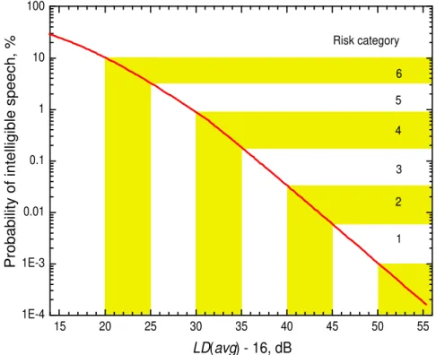
15 20 25 30 35 40 45 50 55 1E-4 1E-3 0.01 0.1 1 10 100

Probability of intelligible speech, %

LD(avg) - 16, dB Risk category 6 5 4 3 2 1

Figure 9. The probability of transmitted speech exceeding the threshold of intelligibility (i.e. being understandable) in terms of the measured LD(avg) value.

Some examples help to illustrate how Figure 9 is used to estimate the likelihood of a speech privacy lapse. If we measured LD(avg) to be 46 dB, then Figure 9 would indicate that there would be about a 1% probability of the meeting room speech level and the spot-receiver ambient noise level being such that the transmitted speech would be just intelligible. That is, about 1% of the time the transmitted speech would be intelligible to a capable eavesdropper. (This is illustrated in the box showing example #1, below). If our measured LD(avg) were 56 dB, then the probability of a speech privacy lapse would be reduced to 0.03%. Then we would expect speech to be intelligible no more than 0.03% of the time. (This is illustrated in the box with example #2).

(24)

15 20 25 30 35 40 45 50 55 1E-4 1E-3 0.01 0.1 1 10 100 Pr

obability of intelligible speech, %

LD(avg) - 16, dB Risk category 6 5 4 3 2 1 Example #1 Measured LD(avg) = 46 dB

SPI goal = -16 dB (threshold of intelligibility)

LD(avg) – 16 = 30 dB

Percentage of the time speech intelligible (above SPI goal) 1% Risk category #4/5 15 20 25 30 35 40 45 50 55 1E-4 1E-3 0.01 0.1 1 10 100

LD(avg) – 16 = 40 dB

Percentage of the time speech intelligible (above SPI goal) 0.03% Risk category #2/3

The speech and noise level statistics are based on measurements over 10 s intervals. There are 2880 of these 10 s intervals in an 8 hour working day. If speech is intelligible 1% of the time, this would correspond to 28.9 of the 10 s intervals in one working day. However, a

(25)

0.03% probability of speech being intelligible corresponds to this occurring just less than once in an 8-hour working day and hence represents much higher speech security. The results in Figure 9 are broken up into categories with 5 dB intervals of measured

LD(avg) values and are labelled Risk categories. Higher categories relate to higher risks or

probabilities of speech security problems. For the highest category (#6), transmitted speech would be intelligible about 3% to 10% of the time corresponding to very minimal privacy and a high risk of a speech privacy lapse. That is, these conditions are not likely to be speech secure. On the other hand, for the lowest category (#1) transmitted speech would be

intelligible for about 0.001% to 0.005% of the time or approximately once in about 10 working days. These conditions would be highly likely to be speech secure. This near perfect level of privacy would be costly to achieve and is probably much better than is normally required for reasonable levels of speech privacy. The probabilities for all six risk categories can be read off Figure 9 and are also found later in Table 6.

To better appreciate the meaning of the various probabilities of a speech privacy lapse, they are converted to numbers of speech privacy lapses in Table 5. It is seen that while a 1% probability of a privacy lapse corresponds to this happening 28.9 times per working day, a 0.001% likelihood of a speech privacy lapse corresponds to a possible privacy lapse occurring about once every 30 days.

Probability of a speech privacy lapse as % of time room occupied Equivalent number of speech privacy lapses 10% 288.8 / day (approx. 1 / 2 minutes) 1% 28.9 / day 0.1% 2.9 / day 0.01% 0.3 / day (approx. 1 / 3 days) 0.001% 0.03 / day (approx. 1/ 30 days)

Table 5. Risk of speech privacy lapses in terms of percentage of the time they might occur and the equivalent number of speech privacy lapses.

One could strive for extremely speech secure conditions in which transmitted speech is not even audible most of the time. This would correspond to designing for SPI = -22 dB or less which is the threshold of audibility. Since this is 6 dB less than the threshold of intelligibility, the measured LD(avg) would have to be 6 dB larger to offer the same probability of a speech privacy lapse relative to the threshold of audibility.

(26)

The probability of transmitted speech being audible can also be determined from Figure 9 by assuming that the horizontal axis values represent LD(avg)-22 values. For the example of a measured average level difference of 56 dB, LD(avg)-22 would equal 34 dB and the

probability of transmitted speech being audible would be about 0.25%. (This is illustrated in the box with Example #3). Of course, for the same construction and LD(avg) value,

transmitted speech is more likely to be audible than intelligible. Similarly a particular probability of speech being audible (percentage risk) represents better conditions than the same probability of speech being intelligible. That is, the probability of a speech privacy lapse and the risk categories on these figures can be either in terms of the audibility of transmitted speech or in terms of the intelligibility of transmitted speech depending on the particular needs for privacy.

15 20 25 30 35 40 45 50 55 1E-4 1E-3 0.01 0.1 1 10 100

Probability of audible speech, %

SPI goal = -22 dB (threshold of audibility)

LD(avg) – 22 = 34 dB

Percentage of the time speech audible (above SPI goal) 0.25% Risk category #4

(27)

4. Designing the Architectural Speech Security of a

Meeting Room

(a) Estimating Level Difference Values at the Design Stage

For existing meeting rooms speech privacy can be measured as described in the previous chapter. However, it is also necessary to be able to predict the expected speech privacy at the design stage. This can be done in terms of equations similar to equations (2.2) and (2.4) which relate the SPI to measured level differences, LD(avg), and some speech and noise level combination. Unfortunately, at the design stage measured level differences are not available and must be determined from available information.

Conventionally, sound transmission characteristics are given in terms of sound transmission loss values, TL, obtained from standard reverberation chamber tests such as the ASTM E90 test. TL(f) values are measured as a function of 1/3 octave band frequency and are often summarised in terms of a single number rating called the Sound Transmission Class, STC.

TL(f) values indicate the attenuation of sound energy on transmission through walls and

other constructions mounted between two reverberant test chambers. TL(f) values are widely available for many different walls, floor-ceilings, doors, windows and other construction types and data for a number of common constructions are included in Appendix I. The speech privacy design procedure should therefore be based on the available TL(f) data for various constructions.

The major difference between LD(f) and TL(f) values is that the LD(f) values are influenced by the level of reverberant sound in the receiving space, but TL(f) values are not affected. Because the spot-receiver microphones are usually located close to the test wall (0.25 m), the effect of the acoustical conditions in the receiving space should be quite small. We can assume that TL(avg) values are related to LD(avg) values by some unknown k as follows,

TL(avg) = LD(avg) + k, dB (4.1) Although some texts suggest approximate values for k, these were not found to be

appropriate and in this work values for k were determined experimentally. The experiments [8] measured the TL(f) and LD(f) values for 5 different walls and for a wide range of

receiving space reverberation times. All the LD(f) values involved measurements at spot-receivers at positions located 0.25 m from the test wall. From simple diffuse field theory, we know that the reverberant level, LR, is proportional to a function of reverberation time and

room volume, i.e.

dB , 161 . 0 ) ( 4 log 10 ) ( 60 ⎭ ⎬ ⎫ ⎩ ⎨ ⎧ ∝ V f T f L_R (4.2)

where, T60(f) is the room reverberation time, s,

V is the room volume, m3, and

f is the third octave band centre frequency.

We would expect the difference between TL(avg) and LD(avg) values to relate to reverberant level values, LR(avg), and for simplicity assume a constant of proportionality in equation (4.2) of 1.0.

(28)

Measured differences between TL(avg) and LD(avg) values, that is the k values, are plotted versus the corresponding reverberant sound levels in Figure 10. These results show a regular trend with little scatter and indicate that one could use the mean trend of these measurements to determine appropriate k values within a small fraction of a decibel. However, such

precision is not normally necessary at the design stage.

Although a wide range of reverberant conditions (i.e. LR values) are included in Figure 10,

most are not likely to occur in spaces adjacent to meeting rooms. The two rectangular boxes on Figure 10 indicate the range of values that would occur for an adjacent space similar to a smaller or larger meeting room. The smaller room was assumed to have a volume of 150 m3 with possible reverberation times varying from 0.3 to 1.2 s (average over speech frequencies from 160 to 5k Hz). The larger room was assumed to have a volume of 500 m3 and with reverberation times varying from 0.5 to 1.6 s (averaged over speech frequencies from 160 to 5k Hz). Most smaller rooms would have much smaller average reverberation times than 1.2 s and the range of likely conditions is probably smaller than the possible ranges indicated by the boxes in Figure 10.

Although one could accurately predict particular k values from the regression line of Figure 10, one could also get a close estimate of the k value using Figure 10 and an approximate room reverberation time and room volume. However, for many practical design situations one could simply assume k = –1 dB with a likely error of about ±0.5 dB. That is usually,

LD(avg) ≈ TL(avg) +1, dB (4.3) This relationship will be used to modify expressions in terms of LD(avg) values to be in terms of TL(avg) values for use at the design stage but is only valid for listening positions 0.25 m from the meeting room boundaries.

-14 -12 -10 -8 -6 -4 -2 -2 -1 0 1 2 3 k, dB 10log{4T₆₀/0.161V}, dB Small room Large room

Figure 10. Measurement results to determine the difference between TL(avg) and LD(avg) values, k, versus the reverberant sound level given by 10log{4T60/(0.161V)}.

(29)

Should there be a need for a more precise relationship, the following is the equation of the best-fit line shown on Figure 10.

k = 0.023{10 log[4T60/0.161V]}2 + 0.717{10 log[4T60/0.161V]} + 3.963, dB (4.4) The RMS error of the data points about the regression line in Figure 10 is only ±0.19 dB.

(30)

(b) Evaluating Designs

To evaluate the ability of a proposed construction to provide adequate speech privacy, one must first calculate the average transmission loss, TL(avg), for the construction. TL(avg) is the arithmetic average of the 1/3 octave band TL(f) values from 160 to 5k Hz. Normally, designs will be based on providing conditions where transmitted speech is not intelligible to eavesdroppers. That is, we are aiming for an SPI = -16 dB (or lower) corresponding to the threshold of intelligibility or lower. When equation (4.3) is approximately correct, then the right hand side of equation (2.4) can be written in terms of TL(avg) values rather than in terms of measured LD(avg) values. That is, using equation (4.3) to substitute for LD(avg) values, equation (2.4) can be re-written as,

dB , 15 ) avg ( ) avg ( ) avg ( −L =TL − L_s _n (4.5)

This makes it possible to re-plot Figure 9 with the horizontal axis labelled as showing

TL(avg) –15 values as in Figure 11. By subtracting 15 from the TL(avg) value, one can use

Figure 11 to indicate the probability of transmitted speech being intelligible to an eavesdropper. 15 20 25 30 35 40 45 50 55 1E-4 1E-3 0.01 0.1 1 10 100

TL(avg) - 15, dB Risk category 6 5 4 3 2 1

Figure 11. The probability of transmitted speech exceeding the threshold of intelligibility (i.e. being understandable) in terms of the expected TL(avg) value.

As an example, consider the case of a TL(avg) value of 45 dB. As illustrated in the box for Example #4, (see box on following page) for a construction with this TL(avg), we would expect transmitted speech to be just intelligible about 1% of the time to a capable

eavesdropper.

For more critical situations, we can also predict the likelihood of the transmitted speech being just audible. In this case we would design for an SPI of –22 dB corresponding to the threshold of audibility. As in the case of measurements in the previous chapter, we can

(31)

predict the probability of transmitted speech being just audible by changing the horizontal axis label of Figure 11 to be TL(avg)-21 values. For a construction with a TL(avg) of 55 dB, Example box #5 shows that we would expect transmitted speech to be just audible only 0.15% of the time. 15 20 25 30 35 40 45 50 55 1E-4 1E-3 0.01 0.1 1 10 100

Probability of audible speech, %

TL(avg) - 21, dB Risk category 6 5 4 3 2 1 Example #5 Predicted TL(avg) = 55 dB

SPI goal = -22 dB (threshold of audibility)

TL(avg) – 21 = 34 dB

Percentage of the time speech audible (above SPI goal) 0.15% Risk category #3 15 20 25 30 35 40 45 50 55 1E-4 1E-3 0.01 0.1 1 10 100 Probabilit y of int elligible speech, % TL(avg) - 15, dB Risk category 6 5 4 3 2 1 Example #4 Predicted TL(avg) = 45 dB

TL(avg) – 15 = 30 dB

Percentage of the time speech intelligible (above SPI goal) 1.0% Risk category #4/5

(32)

Figures 9 and 11 included six privacy risk categories. These are intended to make it easier to focus in on the range of conditions needed for particular situations. For example, meeting rooms where speech privacy is of critical importance could be required to meet risk category #2. A less critical situation might be required to meet category #3 conditions or even to be intermediate to risk categories #3 and #4.

The six risk categories are defined more completely in Table 6. Column 1 lists the six categories. Next the upper and lower TL(avg) values for each category are given in terms of meeting either the threshold of intelligibility (column 2) or meeting the threshold of

audibility (column 3). Column 4 lists the probability of a privacy lapse if the design meets the corresponding TL(avg) values. These probabilities give the percentages of the time that transmitted speech is expected to be either intelligible or audible depending on which

TL(avg) value is used. In the last four columns these probabilities are converted to more

easily recognized frequencies of occurrence such as the number of times per hour, per day, per week or per year. For clarity only selected values are listed.

Risk

category TL(avg), dB _{Intelligibility} TL(avg), dB _Audibility Probability _{of lapse} _hourPer Per _day _weekPer _yearPer

35 41 10% 37 40 46 3.3% 12 45 51 0.89% 3.2 26 50 56 0.18% 0.7 5.3 26 55 61 0.034% 1.0 4.8 60 66 0.0059% 0.85 43 6 < 5 < 4 < 3 < 2 < 1 < 65 71 0.0010% 7.5

Table 6. TL(avg) boundaries for the six risk categories and the corresponding probabilities of transmitted speech being audible or intelligible.

As an example, when designing to minimize the intelligibility of transmitted speech, risk category #4 includes TL(avg) values from 45 to 50 dB in column 2. These values would correspond to a range of probabilities of the transmitted speech being intelligible from 0.18% to 0.89%. These probabilities are then seen to be equivalent to transmitted speech being intelligible between 0.7 and 3.2 times per hour. At the same time this range of probabilities would apply for the audibility of speech but for the range of TL(avg) values from 51 to 56 dB as given in column 3.

(33)

(c) Predicting SPI for Specific Speech and Noise Levels

The previous section described how to estimate the probability of a particular TL(avg) value being acceptable either in terms of intelligibility or in terms of audibility. For example, Figure 11 indicates the probability of transmitted speech being intelligible for various

TL(avg) values, (that is, when the transmitted speech exceeds the threshold of intelligibility

for those conditions). One could alternatively design to meet a particular SPI value using one of several pairs of source-room average speech levels and spot-receiver ambient noise levels. This approach is explained in this section.

We know (see Figure 7) that the larger the difference between the source-room speech level and the spot-receiver ambient noise level, the less often this combination is likely to occur. Thus, if we design to meet the threshold of intelligibility for a very large difference between the source-room speech level and the spot-receiver ambient noise level, the design will correspond to a higher degree of speech security than would a design based on a smaller difference. By creating a set of pairs of equally probable source-room speech level and spot-receiver ambient noise level, we can select the pair that relates to the amount of risk of a speech privacy lapse that is acceptable for a particular design. Table 7 provides 7 different pairs of source-room speech level and spot-receiver ambient noise level (Sn, Nn) with the probabilities of them occurring varying from very rarely to quite often. To ensure a wide range of probabilities, pairs S1, N1 to S6, N6 were selected to correspond to the mid points of each of the speech privacy risk categories on Figure 11 and Table 6. By referring back to Table 5, the probabilities of transmitted speech being intelligible in Table 7 are seen to vary from about once per 14 days (0.0025%) to once per minute (17.1%). Speech and noise pair S7, N7 corresponds to an even lower level of speech privacy. The corresponding TL(avg) and approximate STC values were determined assuming one is designing to meet thresholds of intelligibility. The STC values are approximate estimates from TL(avg) values with an

Table 7. Pairs of equally probable source-room sp

uncertainty of about ±4 STC points.

eech levels (Sn) and spot-receiver ambient noise levels (Nn) with different probabilities of occurring.

Frequency S7 N7 S6 N6 S5 N5 S4 N4 S3 N3 S2 N2 S1 N1 dBA 57.7 40.2 59.9 37.9 62.0 35.8 64.0 33.7 66.2 31.5 68.0 29.5 70.2 27.2 160 41.0 40.4 43.7 38.1 46.5 35.9 49.1 33.5 51.5 30.9 53.9 28.3 56.2 25.6 200 45.7 38.8 48.4 36.5 51.2 34.3 53.8 31.9 56.2 29.3 58.6 26.7 60.9 24.0 250 49.7 37.1 52.4 34.8 55.2 32.6 57.8 30.2 60.2 27.6 62.6 25.0 64.9 22.3 315 48.0 35.4 50.7 33.1 53.5 30.9 56.1 28.5 58.5 25.9 60.9 23.3 63.2 20.6 400 51.1 33.8 53.8 31.5 56.6 29.3 59.2 26.9 61.6 24.3 64.0 21.7 66.3 19.0 500 53.4 32.1 56.1 29.8 58.9 27.6 61.5 25.2 63.9 22.6 66.3 20.0 68.6 17.3 630 51.4 30.4 54.1 28.1 56.9 25.9 59.5 23.5 61.9 20.9 64.3 18.3 66.6 15.6 800 48.3 28.8 51.0 26.5 53.8 24.3 56.4 21.9 58.8 19.3 61.2 16.7 63.5 14.0 1000 46.8 27.1 49.5 24.8 52.3 22.6 54.9 20.2 57.3 17.6 59.7 15.0 62.0 12.3 1250 47.8 25.4 50.5 23.1 53.3 20.9 55.9 18.5 58.3 15.9 60.7 13.3 63.0 10.6 1600 45.8 23.8 48.5 21.5 51.3 19.3 53.9 16.9 56.3 14.3 58.7 11.7 61.0 9.0 2000 41.3 22.1 44.0 19.8 46.8 17.6 49.4 15.2 51.8 12.6 54.2 10.0 56.5 7.3 2500 40.6 20.4 43.3 18.1 46.1 15.9 48.7 13.5 51.1 10.9 53.5 8.3 55.8 5.6 3150 40.2 18.8 42.9 16.5 45.7 14.3 48.3 11.9 50.7 9.3 53.1 6.7 55.4 4.0 4000 39.3 17.1 42.0 14.8 44.8 12.6 47.4 10.2 49.8 7.6 52.2 5.0 54.5 2.3 5000 35.8 15.4 38.5 13.1 41.3 10.9 43.9 8.5 46.3 5.9 48.7 3.3 51.0 0.6 dB(avg) 45.4 27.9 48.1 25.6 50.9 23.4 53.5 21.0 55.9 18.4 58.3 15.8 60.6 13.1 Ls(avg)-Ln(avg) Probability, % Risk category TL(avg) Approx. STC* 3 2 1 7 6 5 4 37.5 42.5 47.5 32.5 37.5 42.5 47.5 52.5 57.5 62.5 17.5 22.5 27.5 32.5 0.079 0.014 0.0025 27.2 32.4 37.6 42.9 48 53.3 58.5 17.13 5.94 1.74 0.42

(34)

By re-arranging equation (4.5) as equation (4.6), we can calculate TL(avg) values for

combinations of Ls(avg) and Ln(avg). This was done for each of the seven pairs of speech and

are noise levels in Table 7 to obtain the TL(avg) values in this table. These TL(avg) values the minimum values for the particular speech and noise levels that just correspond to the threshold of intelligibility. The probabilities of each pair of source-room speech level and spot-receiver ambient noise level occurring were obtained from Figure 11.

dB , 15 ) avg ( ) avg ( ) avg ( = L_s −L_n + TL (4.6)

If we think of the probabilities noise pair occurring as levels of risk, then

w e 7 corresponding to the level of risk that can

of the speech and e can select a speech and noise pair from Tabl

be accepted for a particular design. Then for that level of risk, Table 7 indicates the required construction in terms of its TL(avg) value.

(35)

(d) Errors Due to Using Single Number Ratings such as TL(avg)

and STC

The results in Table 7 are based on average values of various quantities over the frequencies from 160 to 5k Hz. This simplification was introduced in equation (2.3) and has been a part of most calculations in this report. It does lead to small errors because in making this assumption, the clipping of 1/3 octave band signal-to-noise ratios to no lower than –32 dB included in the definition of the SPI measure, is ignored. These small errors are largest for lower speech levels. Transmitted speech levels are lower for the lower speech level combinations in Table 7 and for all cases at higher frequencies. The result is that for the lower speech level cases in Table 7 the calculated TL(avg) values are ~1 dB higher than they would be if the approximations using averages over frequency were not made.

These small errors can be avoided by calculating the required transmission characteristics from 1/3 octave band information rather than using the frequency average values. This was done using the laboratory sound transmission loss data for 250 walls of types that might be found in meeting rooms. SPI values were calculated using equation (2.2) and five of the speech and noise pairs from Table 7 (#1 to #5). TL(f) values were converted to LD(f) values using equation (4.3). The resulting plot of SPI values versus TL(avg) values is shown in Figure 12 and does include the correct clipping of 1/3 octave band signal-to-noise ratios. This graph shows that for a wide range of conditions SPI values are approximately linearly related to TL(avg) values and the scatter about the best fit lines is quite small (standard deviation about the regression line ±0.4 dB). For lower SPI values the relationships become non-linear because of the clipping of signal-to-noise ratios to –32 dB.

This demonstrates that for pairs of source-room speech level and spot-receiver ambient noise level, SPI values can generally be quite accurately predicted from TL(avg) values. Figure 12 also gives a good overview of the relationships between audibility and intelligibility of transmitted speech and the TL(avg) values of walls. This can best be explained with an example. If we consider the case of a speech and noise level difference that is only exceeded 0.014% of the time (second highest data set in Figure 12, risk category #2), then a wall with a

TL(avg) of 57 dB just meets the threshold of intelligibility. That is, for the wall with

TL(avg)= 57 dB, transmitted speech would be expected to be intelligible only 0.014% of the

time. This corresponds to approximately once every two days and represents a very high degree of speech security. Figure 12 also indicates that this same wall (with TL(avg) = 57 dB) would provide barely audible conditions for 0.079% of the time (the third lowest data set on Figure 12. This corresponds to transmitted speech being just audible for approximately 2 times per day. Thus Figure 12 gives a more complete picture by providing information on both the probable intelligibility and audibility of transmitted speech for various constructions.