HAL Id: inria-00516014
https://hal.inria.fr/inria-00516014
Submitted on 8 Mar 2011
HAL is a multi-disciplinary open access
archive for the deposit and dissemination of
sci-entific research documents, whether they are
pub-lished or not. The documents may come from
teaching and research institutions in France or
abroad, or from public or private research centers.
L’archive ouverte pluridisciplinaire HAL, est
destinée au dépôt et à la diffusion de documents
scientifiques de niveau recherche, publiés ou non,
émanant des établissements d’enseignement et de
recherche français ou étrangers, des laboratoires
publics ou privés.
A Refinement-Based Validation Method for
Programmable Logic Controllers
Hai Wan, Xiaoyu Song, Gang Chen, Ming Gu
To cite this version:
Hai Wan, Xiaoyu Song, Gang Chen, Ming Gu. A Refinement-Based Validation Method for
Pro-grammable Logic Controllers. The 10th International Conference on Quality Software, Jul 2010,
Zhangjiajie, Hunan, China. �inria-00516014�
A Refinement-Based Validation Method for
Programmable Logic Controllers
Hai Wan
Key Lab for ISS of MOE, School of Software, Tsinghua University,
Beijing, China
Xiaoyu Song
ECE Dept, Portland State University
Portland, USA
Gang Chen
Lingcore Laboratory Portland, USA
Ming Gu
Key Lab for ISS of MOE, School of Software, Tsinghua University
Beijing, China
Abstract—Programmable logic controllers (PLCs) are widely used in computer-based industrial applications. Timers play a pivotal role in PLC real-time embedded system applications. The paper addresses the formal validation of PLC systems with timers in the theorem proving system Coq. The timer behavior is characterized formally. A refinement validation methodology is presented in terms of an abstract model and a concrete model. The refinement is calibrated by a mapping relation. The soundness of the methodology is shown in the proving system. An illustrative case study demonstrates the effectiveness of the approach.
I. Introduction
Programmable logic controllers (PLCs) are widely used for safety critical applications in various industrial fields. The correctness and reliability of PLC programs are of great importance. Two distinguished features of PLCs programs are the use of timers and the cyclic behavior. In our previous work [1], we formally modeled and proved the correctness of a PLC program with timer control. The behavior of the program is represented by a set of sequences of systems states. Timers are explicitly modeled by a set of axioms over sequences. The model is at the scan cycle level, which means that at the beginning of each scan cycle, a system state is sampled to form the sequence. When compared to the rung level model (i.e., a system state is sampled before the execution of each rung to form a sequence), the scan-cycle level model is an abstract model. In [1], five assumptions and constraints are proposed to ensure the correctness of the abstract model (scan-cycle level model), but the correctness is not formally proved. In this paper, we continue our work: the correctness of the abstract model is formally proved in the theorem proving system Coq based on translation validation.
Translation validation [2] is an approach to the verification of translators. It is deployed to check whether the generated code is a correct implementation of the source code. In this paper we adopt this approach to prove the correctness of the abstract model according to a concrete model. The key to prove the correctness is to find a refinement relation between the two models. In order to establish the refinement relation, as described in [2], we need a common semantic framework for the representations of models is needed and a formal definition of refinement relation. Because of the real-time nature and real-time related properties of PLC programs, we
adopt an extension of synchronous transition system that can express time. We use timed execution sequences [3] as the common semantic base for the concrete and abstract models. The behavior of the concrete (or abstract) model is modeled by a set of timed execution sequences. The notion of refinement is then defined as a relation among sequences from the two sets. In this paper, the five assumptions and constraints are formally defined. And it is shown that they are enough to ensure the correctness of the abstract model.
The rest of the paper is organized as follows. In section I-A we summarize the related works. The formal definitions of the computational model and refinement relation is given in section II. The principles of modeling PLC programs with timers as well as the outline of how to prove the refinement relation are described in detail in section III. Finally section IV concludes the paper.
A. Related Works
There are already a lot of works dealing with the modeling and verification of PLC programs [4][5][6]. To the best of our knowledge, the work that is most close to ours is [7]. In [7], the authors employ translation validation for code-generators of PLCs. Compared to their work, our definition of refinement relation is different in two ways. First they do not have the sampling function. The introduction of sampling function helps to build a refinement relation between two models and ensure that the cyclic behavior of PLCs is modeled. Second they have a constraint that the initial states of the abstract model are mapped to a subset of the initial states of the concrete model.
II. The Computation Model and the Refinement Relation Let V be a set of variables. A state s is a type-consistent valuation of variables in V. Given a variable v ∈ V and a state s, s[v] denotes the value of v at s. The set of all states over V is denoted by P. We adopt the definition of synchronous transition systems in [2] with some modifications.
Definition 1: The following components define a syn-chronous transition system(STS) S = (V, Θ, ρ):
• V ⊆ V: A finite set of system variables.
Φ(sf(i)),Tf(i)
sf(i),Tf(i)
Φ(sf(i+1)),Tf(i+1)
sf(i)+1,Tf(i)+1 sf(i+1),Tf(i+1)
Fig. 1. The refinement relation between sequences
• ρ : A transition relation. ρ is a predicate over two states.
Given two states s and s0, ρ(s, s0)= true iff s0is a possible successor state of s.
Before we introduce the additional time-related predicates, we define the timed state sequences.
Definition 2: A timed state sequence is a 2-tuple (σ, T ) where σ an infinite state sequence and T is an infinite time sequence satisfying monotonicity, i.e., ∀i ≥ 0 Ti+1 ≥ Ti, and
progress, i.e., ∀n ∈ N, ∃i ≥ 0, Ti> n.
A time related predicate is a predicate over timed state sequences.
Definition 3: A timed synchronous transition system (TSTS) is a 2-tuple (S , P) where S is an STS and P is a set of time related predicates.
Given a TSTS A = (S, P) where S = (V, Θ, ρ), a timed execution sequence of A is a timed state sequence (σ, T ) satisfying :
• Initiation: Θ(σ0) holds.
• Consecution: ∀i ∈ N, ρ(σi, σi+1) holds. • Timing Relation: ∀p ∈ P, p(ς) holds.
The set of all timed execution sequences is denoted by ||A||. A PLC program can be modeled by a TSTS. The non-time-related part of the program can be modeled by an STS, while the time-related part can be modeled by a set of time related predicates.
The refinement relation between two TSTSs is given below based on their timed execution sequences.
Definition 4: Given two TSTSs A and C, and two functions: a sampling function f : N → N satisfying ∀i : N, f (i) < f (i+1) and a state mapping function φ :P
C→PA, C is a refinement
of A relative to f and φ iff ∀(σC, TC) ∈ ||C||.∃(σA, TA) ∈
||A||.∀i ∈ N, φ(σC( f (i)))= σA(i) ∧ TC( f (i))= TA(i).
Definition 5 is illustrated graphically in Fig. 1. Intuitively, given f , φ as described above and a timed execution sequence (σ, T ) of the concrete model, { f (0), f (1), · · · } are the sam-pling points along the concrete sequence. After samsam-pling, we obtain a timed state sequence (σf(0)σf(1)· · ·, Tf(0)Tf(1)· · · ).
By applying φ to each state of the first part of the timed state sequence, we would obtain a timed execution sequence (φ(σf(0))φ(σf(1)) · · · , Tf(0)Tf(1)· · · ) of the abstract model.
Definition 5: For systems A and C, A refines B iff there exists two functions f and φ such that C is a refinement of A relative to f and φ.
The problem of checking the correctness of the abstract model turns to a problem of finding a proper sampling function and a proper state mapping function between the abstract
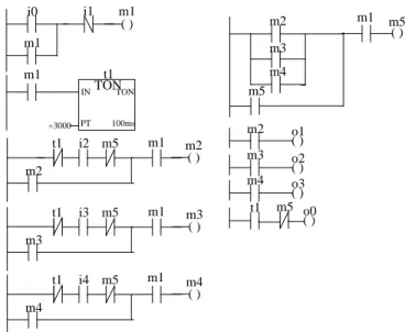
i0 m1 m1 INTON t1 +3000 PT m1 t1 i2 m2 100ms TON m5 m2 m2 m3 m4 m5 ( ) m5 ( ) m2 o1 ( ) m3 o2 ( ) m4 o3 ( ) t1 m5 o0 i1 ( ) ( ) m1 t1 i3 m3 m5 m3 ( ) m1 t1 i4 m4 m5 m4 ( ) m1 m1
Fig. 2. The Example Ladder Diagram
model and the concrete model and prove they satisfy the property in definition 5.
III. Modeling and Verification of PLC Programs with Timers In this section, we show how to build a rung level model of the example program and how to prove the soundness of the scan-cycle level model according to the rung level model. The example PLC program is shown in Fig. 2. For an introduction of PLC, timers and the scan-cycle level model of the example program, because of the limit of space, please refer to [1]. A. Modeling PLC Programs
1) Variables: All relays used in the program are boolean, so they are modeled by variables of type nat → Prop. Since the model is at the rung level, there is a special variable pc (i.e., the program counter) of type nat → location that is used to indicate the current rung under execution. location is inductively defined, but it can be understood as a set {e1· · · e11}
among which e11 denotes the input/output action and for each
i ∈ {1 · · · 10}, ei represents the i-th rung in the example
program.
Inductive location : Set :=
e11|e1|e2|e3|e4|e5|e6|e7|e8|e9|e10. Definition Var := nat -> Prop. Variable pc : nat -> location.
Then, we have the following definitions of variables. Each variable corresponds to a relay of the example program.
Variables i0 i1 i2 i3 i4 m1 m2 m3 m4 m5 o0 o1 o2 o3 t1: Var.
2) Non-Time-Related Part: As mentioned before, the non-time-related part can be modeled by an STS. An STS consists of two parts : the initiation condition and the consecution condition. The initiation condition initial states c states the property that the first state of a sequence should satisfy. And the consecution condition next states c expresses the property that two adjacent states should satisfy.
Definition initial_condition_c
˜i0/\˜i1/\˜i2/\˜i3/\˜i4/\˜m1/\˜m2/\˜m3/\˜m4/\˜m5 /\˜o0/\˜o1/\˜o2/\˜o3/\pc=e11/\˜t1.
Definition next_condition_c
(i0 i1 i2 i3 i4 m1 m2 m3 m4 m5 o0 o1 o2 o3:Prop) l (t1 i0’ i1’ i2’ i3’ i4’ m1’ m2’ m3’ m4’ m5’ o0’
o1’ o2’ o3’:Prop)l’ t1’:= match l with e11=> l’ =e1/\pres(V\{i0,i1,i2,i3,l}) |e1=>m1’=((m1\/i0)/\˜i1)/\l’=e2/\pres(V\{m1,l}) |e2=> l’=e3/\pres(V\{t1,l}) |e3=> m2’=((m2\/(˜t1/\i2/\˜m5))/\m1)/\l’=e4 /\pres(V\{m2,l}) |e4=> m3’=((m3\/(˜t1/\i3/\˜m5))/\m1)/\l’=e5 /\pres(V\{m3,l}) |e5=> m4’=((m4\/(˜t1/\i4/\˜m5))/\m1)/\l’=e6 /\pres(V\{m4,l}) |e6=> m5’=((m2\/m3\/m4\/m5)/\m1)/\l’=e7 /\pres(V\{m5,l}) |e7=> o1’=m2/\l’=e8/\pres(V\{o1,l}) |e8=> o2’=m3/\l’=e9/\pres(V\{o2,l}) |e9=> o3’=m4/\l’=e10/\pres(V\{o3,l}) |e10=> o0’=(t1/\˜m5)/\l’=e11/\pres(V\{o0,l}) end.
Hypothesis initial_states_c : initial_condition_c (i0 0)(i1 0)(i2 0)(i3 0)(i4 0)(m1 0)(m2 0)(m3 0) (m4 0)(m5 0)(o0 0)(o1 0)(o2 0)(o3 0)(pc 0)(t1 0). Hypothesis next_states_c : forall p,
next_condition_c (i0 p)(i1 p)(i2 p)(i3 p)(i4 p) (m1 p)(m2 p)(m3 p)(m4 p)(m5 p)(o0 p)(o1 p)(o2 p) (o3 p)(pc p)(t1 p)(i0 (S p))(i1 (S p))(i2 (S p)) (i3(S p))(i4(S p))(m1(S p))(m2(S p))(m3(S p)) (m4(S p))(m5(S p))(o0(S p))(o1(S p))(o2(S p)) (o3(S p))(pc(S p))(t1(S p)).
3) Time-Related Part: First we need to attach a time to each state in the sequence. This is done by function f c that is monotonous.
Definition Time := nat. Variable fc : nat -> Time.
Hypothesis fc_monotonic : forall p, fc p < fc (S p).
A TON-timer is modeled by three hypotheses that constitute the time related predicates part of the TSTS:
• Reset. If pc = e2, which means the timer rung is
executed, and the timer is not enabled, then the timer bit is false at next state.
Hypothesis h_t1_reset_c:forall p,pc p = e2 -> ˜m1 p->˜t1(S p).
• Set. Given two indexes p1and p2, where pc p1= pc p2 =
e2. If the time interval between them is greater than or
equal to the preset time of the timer and the timer is enabled during this period, then the timer bit is true at next position.
Hypothesis h_t1_set_c : forall p1 p2,pc p1=e2-> pc p2 = e2 ->t1_PT_c <= fc p2 - fc p1 -> being_true_c m1 p1 p2 e2 pc->t1(S p2).
• Set Reverse. If the timer bit is true at position p2and the
timer instruction was executed at the previous position, then there exists a position p1 before p2 such that the
time interval between pred p1 and p2 is great than or
equal to t1 PT cand during this period it is enabled.
Hypothesis h_t1_true_c:forall p2,pc(pred p2)=e2-> t1 p2->exists p1,pc p1=e2/\t1_PT_c<=fc(pred p2) -fc p1/\being_true_c m1 p1 (pred p2) e2 pc.
Finally we have the TSTS for the concrete model.
B. Outline of Refinement Proof
As mentioned in section II, we first need to define two functions: one is a state mapping φ from the concrete states to the abstract states and the other is a sampling mapping f of type N → N. These two functions are used to construct an abstract sequence from a concrete one. We need to prove that the obtained abstract sequence is a timed execution sequence of the abstract model. In order to do so, it is sufficient to prove that the obtained abstract sequence satisfies the initiation condition, consecution condition and the timing relation of the abstract model.
Since the variables used in the two models are the same, φ is an identical function and is omitted.
1) Defining f : Given a natural n, f n is the index of the state in the concrete sequence corresponding to the n-th state in the abstract sequence. f is built using the method proposed in [8] that utilizes a predicate which indicate whether the sampling operation can take place. P is the predicate that is true when the program counter is e11. Intuitively, f n denotes
the index at which P is true for the n-th time. abs is a help function which maps a concrete sequence to an abstract one using the sampling function f .
Definition P n := pc n = e11.
Definition f_mapping_0_to_Prop (x:nat)(P:nat->Prop):= (forall x’, x’ < x -> ˜ P x’) /\ P x.
Definition f_mapping_0_to :=
epsilon nat_non_empty (f_mapping_0_to_Prop P). Definition f_mapping_S_n_to_Prop (n x:nat)(P:nat->Prop)
:=(forall x’, n<x’<x->˜P x’) /\ P x /\ (n < x). Definition f_mapping_S_n_to(n:nat):=
epsilon nat_non_empty(f_mapping_S_n_to_Prop n P). Fixpoint f (n : nat) := match n with
0 => f_mapping_0_to
| S p => f_mapping_S_n_to (f p) end.
Definition abs(T:Type)(v:Var_c)(n:nat):= v(f n).
2) Stating the Assumptions and Constraints: The assump-tions and constraints described in [1] are formally stated. We take three of them for example:
• The executions of the same instruction take the same time.
Hypothesis ExeSameTime :
forall i1 i2 l, pc i1 = l /\ pc i2 = l -> f (S i1) - f i1 = f (S i2) - f i2.
• There is no loop in one scan cycle.
Hypothesis NoLoop :
forall i1 i2, P i1 /\ P i2 -> forall i3 i4, i1 < i3 < i2 /\ i1 < i4 < i2 /\ i3 <> i4 ->
pc i3 <> pc i4.
• Each relay can be set value at most once per scan cycle.
Hypothesis SetOnceM1 :
forall i1 i2, P i1 /\ P i2 -> forall i3 i4, i1 < i3 < i2 /\ i1 < i4 < i2 /\
m1 (S i3) <> m1 i3 /\ m1 (S i4) <> m1 i4 -> i3 = i4.
3) Initiation Condition: Given a timed state sequence ςC
of C, we need to prove that ςA = φ ◦ ςC ◦ f is a sequence
satisfying ΘA(pro j1(ςA(0)). pro j1 is a function to get the
first element of a pair. The theorem is stated as follow and initial condition ais the initiation condition of the abstract model.
initial_condition_a (abs i0 0)
(abs i1 0)(abs i2 0)(abs i3 0)(abs i4 0)(abs m1 0) (abs m2 0)(abs m3 0)(abs m4 0)(abs m5 0)(abs o0 0) (abs o1 0)(abs o2 0)(abs o3 0)(abs t1 0).
4) Consecution Condition: Given a timed state sequence ςC of C, we need to prove that ςA= φ ◦ ςC◦ f is a sequence
satisfying ∀i ∈ N, ρA(pro j1(ς(i), pro j1(ς(i+ 1)). The theorem
about the consecution is stated below. And next condition a is the consecution condition of the abstract model.
Theorem concrete_sequence_sat_abs_next_condition : forall p, next_condition_a(abs i0 p)(abs i1 p) (abs i2 p)(abs i3 p)(abs i4 p)(abs m1 p)(abs m2 p) (abs m3 p)(abs m4 p)(abs m5 p)(abs o0 p)(abs o1 p) (abs o2 p)(abs o3 p)(abs t1 p)(abs i0(S p))(abs i1 (S p))(abs i2(S p))(abs i3(S p))(abs i4(S p)) (abs m1(S p))(abs m2(S p))(abs m3(S p))(abs m4(S p)) (abs m5 (S p))(abs o0(S p))(abs o1(S p))(abs o2(S p)) (abs o3(S p))(abs t1(S p)).
5) Timing Relation: This proof of this result is done based on the theorems describing constraints and time related predi-cates of ||A||. If we prove the theorems directly on the concrete model, a lot of irrelevant information will be introduced which makes the proof much more difficult. The theorems about the constraints can help to remove the irrelevant information. In practice, they are useful. The following theorems are about the timed related predicates and are similar to those hypotheses of the abstract model except that each variable is replaced by its abstract version. They are proved based on the theorems of constraints and timed related predicates of the concrete model.
Theorem concrete_sequence_sat_abs_t1_reset: forall c, ˜abs m1 c->˜abs t1
Theorem concrete_sequence_sat_abs_t1_true : forall c2,abs t1 c2->exists c1,
t1_PT <= abs fc (pred c2)-abs fc(pred c1) /\being_true (abs m1) c1 c2.
Theorem concrete_sequence_sat_abs_t1_set : forall c1 c2, t1_PT <= abs fc(pred c2)-abs fc(pred c1)->
being_true (abs m1) c1 c2 -> abs t1 c2.
6) The Final Theorem: The final result is that for all properties that are held by the abstract model are also held by the concrete model according to the sampling function. In the theorem P is a property of the abstract model and sequences of form “abs •” are the sampled sequences. By using this theorem, the properties we have proved in [1] are also satisfied by the concrete model – there is no need to prove them on the concrete model from scratch.
Theorem refinement_relation_property : forall P (f:Cycle->Time)
(i0 i1 i2 i3 i4 m1 m2 m3 m4 m5 o0 o1 o2 o3 t1:Var), (initial_condition_a(i0 0)(i1 0)(i2 0)(i3 0)(i4 0)
(m1 0)(m2 0)(m3 0)(m4 0)(m5 0)(o0 0)(o1 0)(o2 0) (o3 0)(t1 0)) ->
(forall p : Cycle,next_condition_a (i0 p)(i1 p) (i2 p)(i3 p)(i4 p)(m1 p)(m2 p)(m3 p)(m4 p)(m5 p) (o0 p)(o1 p)(o2 p)(o3 p)(t1 p)(i0(S p))(i1(S p)) (i2(S p))(i3(S p))(i4(S p))(m1(S p))(m2(S p)) (m3(S p))(m4(S p))(m5(S p))(o0(S p))(o1(S p)) (o2(S p))(o3(S p))(t1(S p))) ->
(forall c,˜m1 c->˜t1 c)->(forall c1 c2,
t1_PT<=f(pred c2)-f(pred c1)->being_true m1 c1 c2 -> t1 c2) ->(forall c2,t1 c2->
exists c1,t1_PT<=f(pred c2)-f(pred c1)/\ being_true m1 c1 c2)->
P i0 i1 i2 i3 i4 m1 m2 m3 m4 m5 o0 o1 o2 o3 t1)-> P(abs i0)(abs i1)(abs i2)(abs i3)(abs i4)(abs m1) (abs m2)(abs m3)(abs m4)(abs m5)(abs o0)(abs o1) (abs o2)(abs o3)(abs t1).
7) Remarks: After analyze the dependence among theo-rems used in the proof, it can be concluded that the proof of the refinement relation between abstract and concrete time related predicates only uses the theorem of constraints and concrete timed related predicates, which means that the refinement relation between abstract and concrete models are independent of the STS of the concrete model if the concrete model satisfies the constraints. By modifying the source codes or generating codes that satisfy the constraints, the refinement relation between the time related parts is held without proving.
IV. Conclusions
The paper addressed the formal validation of PLC systems with timers in the theorem proving system Coq. The timer behavior is characterized formally. A refinement validation methodology is presented in terms of an abstract model and its interpretation. The interpretation was calibrated by a mapping relation. The soundness of the methodology is shown in the proving system. An illustrative case study demonstrates the effectiveness of the approach.
References
[1] H. Wan, G. Chen, X. Song, and M. Gu, “Formalization and verification of PLC timers in Coq,” in COMPSAC 2009: The 33rd Annual IEEE International Computer Software and Applications Conference, 2009. [2] A. Pnueli, M. Siegel, and E. Singerman, “Translation validation.”
Springer, 1998, pp. 151–166.
[3] T. A. Henzinger, Z. Manna, and A. Pnueli, “Temporal proof method-ologies for timed transition systems,” Inf. Comput., vol. 112, no. 2, pp. 273–337, 1994.
[4] A. Mader, “A classification of PLC models and applications,” in In WODES 2000: 5th Workshop on Discrete Event Systems. Kluwer Academic Publishers, 2000, pp. 21–23.
[5] G. Frey and L. Litz, “Formal methods in PLC programming,” in IEEE International Conference On System Man and Cybernetics, vol. 4, 2000, pp. 2431–2436.
[6] M. Younis and G. Frey, “Formalization of existing PLC programs: A survey,” in Proceedings of CESA, 2003, pp. 0234–0239.
[7] D. Pollmacher, W. Zimmermann, and H.-M. Hanisch, “Translation vali-dation for model-based code-generators for PLCs,” in ETFA, 2005. [8] T. Melham, Higher order logic and hardware verification. New York,