Publisher’s version / Version de l'éditeur:
Vous avez des questions? Nous pouvons vous aider. Pour communiquer directement avec un auteur, consultez la première page de la revue dans laquelle son article a été publié afin de trouver ses coordonnées. Si vous n’arrivez pas à les repérer, communiquez avec nous à [email protected].
Questions? Contact the NRC Publications Archive team at
[email protected]. If you wish to email the authors directly, please see the first page of the publication for their contact information.
https://publications-cnrc.canada.ca/fra/droits
L’accès à ce site Web et l’utilisation de son contenu sont assujettis aux conditions présentées dans le site
LISEZ CES CONDITIONS ATTENTIVEMENT AVANT D’UTILISER CE SITE WEB.
10th International Conference on Computing and Control for the Water Industry,
CCWI 2009 Conference [Proceedings], p. 10, 2009-09-01
READ THESE TERMS AND CONDITIONS CAREFULLY BEFORE USING THIS WEBSITE. https://nrc-publications.canada.ca/eng/copyright
NRC Publications Archive Record / Notice des Archives des publications du CNRC :
https://nrc-publications.canada.ca/eng/view/object/?id=51017034-34ba-4539-b6a6-4893b8cc45dc
https://publications-cnrc.canada.ca/fra/voir/objet/?id=51017034-34ba-4539-b6a6-4893b8cc45dc
NRC Publications Archive
Archives des publications du CNRC
This publication could be one of several versions: author’s original, accepted manuscript or the publisher’s version. / La version de cette publication peut être l’une des suivantes : la version prépublication de l’auteur, la version acceptée du manuscrit ou la version de l’éditeur.
Access and use of this website and the material on it are subject to the Terms and Conditions set forth at
I-WARP: individual water main renewal planner
Kleiner, Y.; Rajani, B. B.
http://www.nrc-cnrc.gc.ca/irc
I -WARP: individua l w a t e r m a in re ne w a l pla nne r
N R C C - 5 2 6 4 0
K l e i n e r , Y . ; R a j a n i , B . B .
S e p t e m b e r 2 0 0 9
A version of this document is published in / Une version de ce document se trouve dans:
10th International Conference on Computing and Control for the Water Industry
- CCWI2009 Conference, Sheffield, UK, September 1-3, 2009, pp. 10
The material in this document is covered by the provisions of the Copyright Act, by Canadian laws, policies, regulations and international agreements. Such provisions serve to identify the information source and, in specific instances, to prohibit reproduction of materials without written permission. For more information visit http://laws.justice.gc.ca/en/showtdm/cs/C-42
Les renseignements dans ce document sont protégés par la Loi sur le droit d'auteur, par les lois, les politiques et les règlements du Canada et des accords internationaux. Ces dispositions permettent d'identifier la source de l'information et, dans certains cas, d'interdire la copie de documents sans permission écrite. Pour obtenir de plus amples renseignements : http://lois.justice.gc.ca/fr/showtdm/cs/C-42
I-WARP: Individual Water Main Renewal Planner
Yehuda Kleiner and Balvant Rajani
National Research Council Canada, Ottawa, Ontario, Canada Abstract
I-WARP is based upon a nonhomogeneous Poisson approach to model breakage rates in individual water mains. The structural deterioration of water mains and their subsequent failure are affected by many factors, both static (e.g., pipe material, pipe size, age (vintage), soil type) and dynamic (e.g., climate, cathodic protection, pressure zone changes). I-WARP allows for the consideration of both static and dynamic factors in the statistical analysis of historical breakage patterns. This paper describes the
mathematical approach and demonstrates its application with the help of a case study. The research project within which I-WARP was developed, was jointly funded by the National Research Council of Canada (NRC), and the Water Research foundation (formerly known as the American Water Works Association Research Foundation - AwwaRF) and supported by water utilities from USA and Canada.
1. Introduction
The use of statistical methods to discern patterns of historical breakage rates and use them to predict water main breaks has been widely documented. Kleiner and Rajani, (2001) provided a comprehensive review of approaches and methods that had been developed prior to their review. Since then, several more methods have been proposed, such as those by Park and Loganathan (2002), Mailhot et al. (2003), Dridi et al. (2005), Giustolisi et al. (2005), Watson et al. (2006), Giustolisi and Berardi (2207), Boxall et al. (2007), Le Gat (2008) and Economou et al. (2008) to name but a few.
Many factors, operational, environmental and pipe-intrinsic factors, jointly affect the breakage rate of a water main. While not all pipes are created equal (even pipes of the same material and size), it is normally assumed that pipes that share a specific intrinsic property, such as material, or diameter, can be expected to have the same breakage pattern, all else being equal. However, non-pipe-intrinsic factors may have varying effect on the breakage patterns of different pipes, even if all else is equal. For example, two pipes of the same material, diameter, age, etc. can be impacted differently by climate. These differences are due to variability for which we may never have enough data to account. At the same time, it is unreasonable to perform a statistical analysis on the breakage pattern of a single pipe because there often are insufficient breaks to conduct a credible analysis. For this reason, the forecasting of breaks in individual water mains has proven to be quite a challenge.
In this paper we present I-WARP (Individual Water mAin Renewal Planner), which is a tool to analyse the historical breakage patterns of individual water mains. I-WARP is based on the assumption that breaks on an individual pipe occur as a non-homogeneous Poisson process (NHPP). NHPP has been suggested by others to model the same phenomenon (e.g., Constantine and Darroch, 1993; Røstum, 2000; Jarrett et al., 2003, among others). The approach proposed here differs from others in that allows for the
consideration of dynamic factors, while existing NHPP approaches consider only static factors (i.e., pipe-intrinsic).
The rest of this paper is organised as follows: Section 2 provides the theoretical background for the model, section 3 discusses issues related to the use of specific covariates, section 4 describes the Zero-inflated Poisson concept, which is provided as an option in I-WARP, Section 5 provides details on the testing and validation of I-WARP results, Section 6 provides a case study to illustrate the model application and section 7 provides summary and conclusions.
2. Non-homogeneous Poisson-based model
In the proposed model we assume that breaks at year t for an individual pipe i are Poisson arrivals with mean intensity λi,t. Therefore, the probability of observing ki,t breaks is given
by ! ) exp( ) ( , , , , , t i t i k t i t i k k P t i λ λ ⋅ − = ] ) ( exp[ , , , t i t i t i o t i α θτ g αz βp γq λ = + + + + (1)
where αo is a constant, τ(gi,t) is the age covariate, and θ is its coefficient, gi,t is the age of
pipe i at year t; zi is a row vector of pipe-dependent covariates (e.g., length, diameter, etc.) and α is a column vector of the corresponding coefficients; pt is a row vector of
time-dependent covariates (e.g., climate) and β is a column vector of the corresponding coefficients; qi,tis a row vector of both pipe-dependent and time-dependent covariates (e.g., number of known previous failure - NOKPF, cathodic protection) and γ is a column vector of the corresponding coefficients. Note that if τ(gi,t) = gi,t then the aging is
exponential, i.e., λ is an exponential function of pipe age, whereas if τ(t) = loge(gi,t) then
λ becomes a power function of pipe age. Year t is taken relative to the first year for which breakage records are available. Coefficients are obtained using the maximum likelihood method.
3. Covariates Pipe-dependent
Pipe-dependent covariates can be considered explicitly in the probabilistic model or implicitly by partitioning the data into homogeneous populations with respect to these covariates. The explicit consideration introduces some limitations. For example, if one includes pipe diameter in the zi vector of covariates the mean breakage intensities for all pipes with the same diameter are assumed to be impacted by the same magnitude. Moreover, this inclusion implies that pipes of different diameters are impacted proportionally to the loge of the ratio between their respective diameters. Alternatively,
one can partition the population of pipes into groups, each comprising only pipes with the same diameter. Each group is then analysed separately, producing group specific
coefficients. The latter approach encompasses two advantages: (a) removal of the forced proportionality described above, and (b) relaxation of the implied assumption that each covariate affects the mean intensity independently. These two advantages come at the
cost of reduced statistical significance due to analysis of smaller pipe populations (groups).
I-WARP uses pipe diameter as a grouping criterion, as well as categorical properties such as pipe material, soil type, service connections or any such property that may be
supported by available data. However, pipe length and pipe cluster are used as explicit covariates in the probabilistic model. Pipe cluster is a surrogate for spatial covariates for which data may not always be available. Water utilities often lack data that are (directly or indirectly) geographically related, such as soil data, overburden characteristics (land development, traffic loading), historical installation practices, groundwater fluctuations, transient pressures, poor bedding, etc. These data, if available, may sometimes help to ‘explain’ variations in breakage rates among individual water mains. In the absence of such data, the proximity of a pipe to a cluster of historical breaks may serve as a useful surrogate. The details on how to form pipe clusters and the cluster covariates are not discussed in this paper.
Time-dependent
In the category of time-dependent covariates, three climate-related covariates were considered, namely freezing index (FI), cumulative rain deficit (RDc) and snapshot rain deficit (RDs). Kleiner and Rajani (2004) provided a detailed introduction and a rational for using these covariates by. FI is a surrogate for the severity of a winter, RDc is a surrogate for average annual soil moisture and RDs is a surrogate for locked-in winter soil moisture (appropriate for cold regions, where soil can freeze in the winter). I-WARP is not restricted in the way it can consider time-dependent covariates. In fact any phenomenon, suspected as a contributor to observed variations in breakage rate, can be considered in the model, provided there exists a time series describing this
phenomenon over the observed period of time. Such phenomena can be represented quantitatively or qualitatively. For example, in one of the case studies documented in this research, uncharacteristically elevated breakage rates were observed in a network during two non-contiguous years.. A quick inquiry revealed that the network experienced pump station failures in those years, which resulted in high breakage rates probably due to transient pressures. A qualitative time series describing this phenomenon was incorporated in the model and the calibration results improved significantly. Pipe and time-dependent
I-WARP considers three pipe-dependent and time-dependent covariates, namely, number of known previous failures (NOKPF), a covariate related to hot spot cathodic protection (HSCP) and a covariate related to retrofit cathodic protection (RetroCP). To ensure stability in the maximum likelihood calculations it may be beneficial to use the loge of
NOKPF as the covariate, especially when there are substantial discrepancies between breakage rates of individual pipes in the group.
The dependency of pipe failure rate on the number of previous failures has been observed by others (e.g., Andreou et al., 1987; Rostum, 2000). Typically, covariates used were break order, or number of breaks observed since installation. As the vast majority of water utilities do not have a complete breakage history of pipes since installation (left truncated data), we selected a more realistically available (if less rigorous) covariate of
previously known number of failures. The aforementioned cathodic protection covariates are not described in this paper
4. The Zero-inflated Poisson (ZIP) process
In reality, most water mains fail relatively rarely, which means that in a typical data set many (if not most) of our data points will have the observed value ki,t = 0 (i.e., zero
breaks observed for pipe i at year t - see equation 1). It has been observed (e.g., Lambert, 1992) that a counting process with many zeros (i.e., many more than what is expected from Equation 1) cannot be adequately represented by a Poisson process. Lambert (1992) proposed a technique she called ‘zero inflated Poisson’ (ZIP) regression, for handling zero inflated count data. In this approach, the counting process at hand is produced simultaneously by two mechanisms, namely a zero generating process and a Poisson process. Economou et al. (2008) used this approach in their model to predict pipe breakage rates, and called the probability of obtaining a zero data point “the natural tendency of the pipe to resist failure”. I-WARP allows the option of incorporating the ZIP process in the analysis, as it can (but is not guaranteed to) improve prediction accuracy. When ZIP is considered the probability of observing ki,t breaks (at year t for an individual
pipe i) becomes T t N i k k e G k e G G k P t i t i k t i t i t i t i t i t i t i t i t i , , 2 , 1 ; , , 2 , 1 0 for ! / ) 1 ( 0 for ) 1 ( ) ( , , , , , , , , , , , K K = = ⎪⎩ ⎪ ⎨ ⎧ > − = − + = − − λ λ λ (2)
where N is the number of pipes and T is the number of years of available breakage data, Gi,t is the parameter of the second mechanism (the first in the Poisson process) that
produces ki,t = 0 with probability Gi,t. It is convenient to formulate Gi,t in a logit form
because its value must lie in the interval [0, 1], i.e.,
) ( ) ( , , 1 or ) covariates some ( ) ( ⋅ ⋅ + = = f f t i t i e e G f G Logit (3)
It is reasonable to assume that Gi,t is generally influenced by the same covariates that
influence the mean intensity λi,t. Therefore we define Gi,t as a function of λi,t
t i t i g g t i e e G , 0 , 0 1 , λ λ − − + = (4)
where go is the ZIP coefficient. Note that with this formulation Gi,t tends to zero as λi,t
increases and Gi,t tends to unity as λi,t decreases.
5. Testing and validating I-WARP
The testing protocol consists of three steps: (a) training the model (discern coefficients) on data of T years (training period), (b) use the discerned coefficients to forecast breaks
in subsequent V years (validation period), and (c) compare the forecasted and observed breaks in the validation period.
The evaluation of how well the trained model fits observed data (step (a)) is challenging for this type of model because observed data are integers (counts of breaks) while the model predicts expected number of breaks (referred to earlier as ‘mean intensity’ or ‘mean rate of occurrence’ of failure), which are real numbers. Therefore, measures like root mean square deviations or generalized R2 (Nagelkerke, 1991) are not well suited for this type of model. Consequently, two goodness of fit measures were used, namely a pipe-dimension coefficient of determination, pR2, and a time-dimension coefficient of determination, tR2.
∑
∑
∑∑
∑
∑
∑
∑
∑
∑∑
∑
∑
∑
= = = = = = = = = = = = = = − − − = − − − = T t T t N i t i N i t i T t N i t i N i t i N i T t N i t i T t t i N i T t t i T t t i k T k k tR k N k k pR 1 2 1 1 , 1 , 1 2 1 , 1 , 2 1 2 1 1 , 1 , 1 2 1 , 1 , 2 ) 1 ( ) ˆ ( 1 ) 1 ( ) ˆ ( 1 λ λ (5)where ki,t is the observed - and λˆi,t is the estimated - number of breaks in pipe i at year t.
Essentially pR2 computes the coefficient of determination between the observed and predicted data, where the data are aggregated by pipe (i.e., for each pipe it compares the total number of observed breaks with predicted values over training period T). Similarly, tR2 computes the coefficient of determination between the observed and predicted data, where the data are aggregated by year (i.e., for each year in T it compares the total number of observed breaks to predicted values in all N pipes).
Equation 5 can also be used to evaluate results of step (c), i.e., the forecasting accuracy. In addition, we used a measure to assess the ‘ranking ability’ (in terms of forecasted number of breaks) of the forecast. This measure is explained as follows: if in a group P, comprising p pipes there is a subset N comprising n pipes that have at least m breaks, if one draws at random n pipes out of P, then P-value is defined as the probability that at least k pipes (from those drawn at random) are members of N. It can be shown that k is a random variable with a hyper-geometric probability distribution, and P-value can thus be computed. For example, suppose that in a group of 100 pipes 5 pipes are observed to have experienced at 4 breaks (each) during the validation period. If 5 pipes are selected at random from the 100 pipes, the probability that at least two of those selected will have 5 breaks in the validation period is P-value ≈ 0.019. It follows that if the model succeeds in identifying 2 out of the 5 highest breaking pipes (in a group of 100 pipes) it is doing significantly better than a random draw (which has only about 2% chance to do as well). The statistical significance of the contribution of each covariate to the model accuracy can be determined by e.g., the likelihood ratio test (e.g., Ansel and Phillips, 1994). This topic, however, is not discussed in this paper.
6. Case study
We use a data set obtained from a water utility in western Canada to illustrate the performance of I-WARP. The data set comprises 1091 individual pipes (each with a minimum length of 20 m) with a total length of 146.6 km, all 150 mm diameter unlined cast iron pipes, installed between 1956 and 1960. Available pipe data included pipe material, diameter, installation year, length, and x-y coordinates of pipe nodes. Any intervention that involved pipe exposure and repair was considered a “break” event, for which date, type and related pipe ID was provided. Full year breakage data were available for the years 1961 – 2006. Some information on cathodic protection was also provided but is not used in this example. Climate data for the analysis years were obtained from Environment Canada. I-WARP was trained on 40 years failure data from 1962 to 2001 and the coefficients obtained from training were used to forecast breaks for validation for the subsequent 5 years, i.e., 2002-2006.
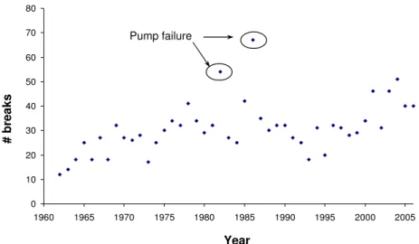
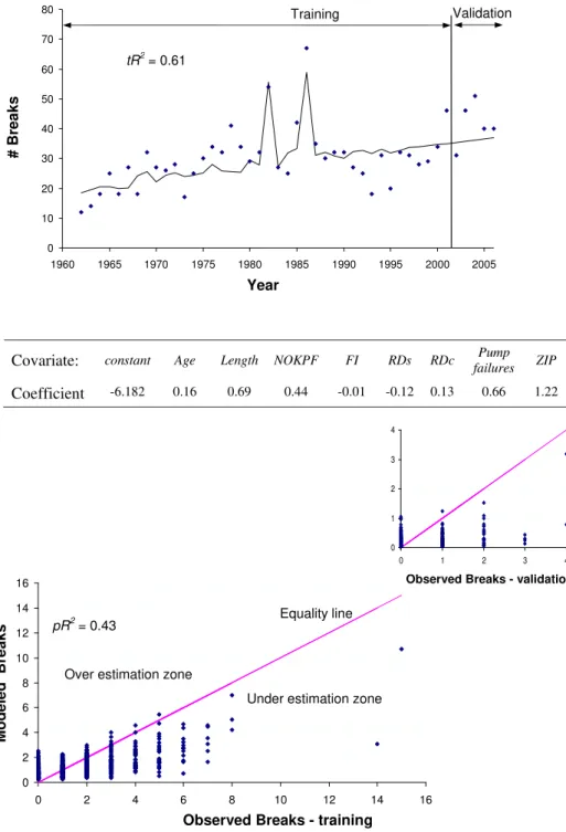
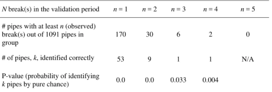
The temporal distribution of the breaks is illustrated in Figure 1. Note the two outliers in 1982 and 1986. The utility engineering staff noted that pumping station failures occurred in these years with the consequence of a significant spike in the number of pipe failures. As discussed earlier, I-WARP allows the inclusion of such information by means of a user-defined time-dependent covariate. Figure 2 illustrates the training and validation results with temporal aggregation (top) and pipe-aggregation (bottom). Table 1 provides the ranking ability of the model. Note that the ranking ability is for the validation (not training) period.
Figure 1. Breaks Aggregated by year
0 10 20 30 40 50 60 70 80 1960 1965 1970 1975 1980 1985 1990 1995 2000 2005 Year # brea ks Pump failure
Covariate: constant Age Length NOKPF FI RDs RDc Pump
failures ZIP
Coefficient -6.182 0.16 0.69 0.44 -0.01 -0.12 0.13 0.66 1.22
Figure 2. Training and validation results
0 10 20 30 40 50 60 70 80 1960 1965 1970 1975 1980 1985 1990 1995 2000 2005 # Brea ks Year tR2 = 0.61 Training Validation 0 2 4 6 8 10 12 14 16 0 2 4 6 8 10 12 14 16
Observed Breaks - training
M o de le d B re a k s Equality line
Over estimation zone
Under estimation zone
pR2 = 0.43
Observed Breaks - validation
0 1 2 3 4 0 1 2 3 4
Table 1. Ranking ability of the model (validation period)
N break(s) in the validation period n = 1 n = 2 n = 3 n = 4 n = 5
# pipes with at least n (observed) break(s) out of 1091 pipes in group
170 30 6 2 0
# of pipes, k, identified correctly 53 9 1 1 N/A
P-value (probability of identifying
k pipes by pure chance) 0.0 0.0 0.033 0.004
The ageing covariate τ(t) = loge(gi,t) was used in this case study. An examination of the
coefficients (Figure 2) reveals that background ageing was therefore proportional to sixth root (power of about 0.16) of pipe age. The impact of climate covariates on the model was inconsistent. Freezing index (FI) showed little impact, rain deficit (RDc) appeared to have a more significant impact, but the impact of snapshot rain deficit (RDs) was in a counter intuitive direction (negative coefficient). Water mains of this water utility are typically buried at a depth of 2.4 m, which may explain the insignificant impact of FI, but not the negative sign of RDs. The positive sign of PKNOF may point to a “worse than old” condition (in repairable systems four repair-related conditions are observed, “good as new”, “good as old”, “better than old” and “worse than old”). The length covariate in this case study was taken as the loge of pipe length, which means that the number of
estimated break was proportional to the length of the pipe raised to the power of 0.7, which is a relatively strong dependency.
The results seem to indicate that in this case study:
• I-WARP tended to be quite accurate in predicting total numbers of breaks:
# Breaks
Training period Validation period
Observed 1184 208
Predicted 1173 189
• I-WARP was rather successful in estimating the total number of breaks per year of the entire group (tR2 = 0.61)
• I-WARP was not as successful in estimating the number of breaks per pipe (pR2 = 0.43). It tended to over-estimate the number of breaks for pipes that experienced few breaks, while under-estimating the number of breaks for those pipes that experienced a higher number of breaks. A similar tendency has been observed by others, e.g., Rostum (2000). This may be due to the fact that there are many pipes with zero or few breaks and only a few pipes with many breaks.
• I-WARP displayed a statistically significant ranking ability in its forecast, which would help to prioritise pipes for renewal.
Formatted: Bullets and Numbering
Additionally, when we varied the length of the validation period we have observed that longer validation periods resulted in improved ranking ability of the forecast. This may be because I-WARP forecasts mean intensities, while observed values are random events. The longer the forecast period the more these observed values would tend towards their means.
7. Summary and conclusions
I-WARP is a non-homogeneous Poisson process-based model, which considers three classes of covariates, pipe-dependent, time-dependent and pipe and time dependent. Some pipe-dependent covariates (e.g., pipe diameter, material, soil type, vintage, etc.) are considered implicitly through pipe grouping, while time-dependent (e.g., climate) and pipe and time dependent (e.g., NOKPF, cathodic protection) covariates are considered explicitly in the statistical analysis.
I-WARP was demonstrated using a case study. The model was trained on 40 years of historical breakage data and the trained model used to forecast breaks in the subsequent 5 years. While prediction of aggregate number of breaks per year was good, the aggregated total number of breaks per pipe was over estimated for pipes with few historical breaks and underestimated for pipes with many historical breaks. Ranking ability was statistically quite significant.
A prototype computer application was created for the application of I-WARP. It will soon be publicly available through WRF.
Acknowledgement
I-WARP was developed as part of a research project, which was co-sponsored by the Water Research Foundation (WRF – formerly known as the American water Works Association Research Foundation – AwwaRF), the NRC and water utilities from the United States and Canada. The authors wish to acknowledge the invaluable help provided by Dr. Ahmed Abdel Akher at the NRC.
References
Andreou, S. A., Marks, D. H., and Clark, R. M. (1987). “A new methodology for modeling break failure patterns in deteriorating water distribution systems: Theory.” Advance in Water Resources, 10, 2-10. Ansell, J.I., and M.J. Phillips, (1994). “Practical methods for reliability data analysis” Oxford University
Press, Oxford, UK.
Boxall, J. B., A. O’Hagen, S. Pooladsaz, A. Saul, and D. Unwin, (2007). Estimation of burst rate in water distribution mains”, Proceedings of the Institution of Civil Engineers, Water Management I60, Issue
WM2, pp 73-82. June.
Constantine, A. G., and Darroch, J. N. (1993). “Pipeline reliability: stochastic models in engineering technology and management.” S. Osaki, D.N.P. Murthy, eds., World Scientific Publishing Co. Dridi, L,. Mailhot, A., Parizeau, M., and Villeneuve J.P. (2005) “A strategy for optimal replacement of
water pipes integrating structural and hydraulic indicators based on a statistical water pipe break model”. Proceedings of the 8th International Conference on Computing and Control for the Water
Industry, U. of Exeter, UK, September, 65-70.
Economou, T., Kapelan, Z. and Bailey, T. (2008), “A Zero-Inflated Bayesian Model for the Prediction of Water Pipe Bursts”, Proc. 10th International Water Distribution System Analysis Conference, CD-ROM edition, Kruger National Park, South Africa.
Giustolisi, O., Laucelli, D, and Savic D. A., (2005). “A decision support framework fro short time planning of rehabilitation”, Proceedings of Computer and Control in Water Industry (CCWI), (1), 39-44.
Giustolisi, O. and L. Berardi, (2007). “Pipe level burst prediction using EPR and MCS-EPR”. Proceedings
of the Combined International Conference of Computing and Control for the Water Industry (CCWI2007) and Sustainable Urban water Management (SUWM2007) on Water Management Challenges in Global Change, Leicester, UK, September, pp. 39-46.
Jarrett, R. O. Hussain, and J. Van der Touw (2003). “Reliability assessment of water pipelines using limited data”, OzWater, Perth, Australia.
Kleiner, Y. and Rajani, B. (2001). “Comprehensive review of structural deterioration of water mains: statistical models”. Urban Water, (3), 131-150.
Kleiner, Y. and Rajani, B. (2004). “Quantifying effectiveness of cathodic protection in water mains: theory,” Journal of Infrastructure Systems, ASCE, 10,(2), 43-51.
Lambert, D. (1992). “Zero-Inflated Poisson regression, with an application to defects in manufacturing”,
Technometrics, Vol. 34, No. 1, pp. 1-14.
Le Gat, Y. (2008). “Extending the Yule Process to model recurrent failures of pressure pipes”,Private communication.
Mailhot, A., A. Paulin, and Villeneuve J-P, (2003). “Optimal replacement of water pipes”, Water
Resources Research, 39, (5), 1136.
Nagelkerke, N. (1991). “A Note on a General Definition of the Coefficient of Determination”, Biometrika, 78(3), pp. 691-692.
Park, S. and G. V. Loganathan (2002). “Optimal pipe replacement analysis with a new pipe break prediction model” Journal of the Korean Society of Water and Wastewater, 16/6, pp. 710-716. Røstum, J. (2000). “Statistical modelling of pipe failures in water networks”. PhD thesis, Norwegian
University of Science and Technology, Trondheim, Norway.
Watson, T.G., C.D. Christian, A. J., Mason, M. H. Smith, and R. Meyer (2004). “Bayesian-based pipe failure model”, Journal of Hydroinformatics, IWA publishing, 06.4, pp 259-264.