Adaptive Statistical Language Modelling
by Raymond Lau
Submitted to the Department of Electrical Engineering and Computer Science in Partial Fulfillment of the Requirements for the Degree of
Master of Science
at the Massachusetts Institute of Technology May 1994
Copyright © 1994, Raymond Lau. All rights reserved.
The author hereby grants to M.I.T. permission to reproduce and to distribute copies of this thesis document in whole or in part,
and to grant others the right to do so.
AA
/'
Author
/
Department of Electrical Engineering and Computer Science
, , \ May,
1994
Certified by Certified by I V - J - _' Victor Zue Thesis Supervisor ISalim Roukos, IBM Thomas J. Watson Research Center '-)l .d, (JA Company Supervisor Accepted by
Department
·_
Adaptive Statistical Language Modelling
byRaymond Lau
Submitted to the Department of Electrical Engineering and Computer Science on May 6, 1994 in partial fulfillment of the requirements for the
Degree of Master of Science in Electrical Engineering and Computer Science
ABSTRACT
The trigram statistical language model is remarkably successful when used in such applications as speech recognition. However, the trigram model is static in that it only considers the previous two words when making a prediction about a future word. The work presented here attempts to improve upon the trigram model by considering additional contextual and longer distance information. This is frequently referred to in the literature as
adaptive statistical language modelling because the model is thought of as adapting to the
longer term information. This work considers the creation of topic specific models, statistical evidence from the presence or absence of triggers, or related words, in the document history
(document triggers) and in the current sentence (in-sentence triggers), and the incorporation
of the document cache, which predicts the probability of a word by considering its frequency in the document history. An important result of this work is that the presence of self-triggers, that is, whether or not the word itself occurred in the document history, is an extremely important piece of information.
A maximum entropy (ME) approach will be used in many instances to incorporate
information from different sources. Maximum entropy considers a model which maximizes entropy while satisfying the constraints presented by the information we wish to incorporate. The generalized iterative scaling (GIS) algorithm can be used to compute the maximum entropy solution. This work also considers various methods of smoothing the information in a maximum entropy model. An inportant result is that smoothing improves performance noticibly and that Good-Turing discounting is an effective method of smoothing.
Thesis Supervisor: Victor Zue
Title: Principal Research Scientist, Department of Electrical Engineering and Computer Science
Table of Contents
Acknowledgm ents ...5
1.0 Introduction and Background ...6
1.1 Language Models ... 6
1.2 Trigram Statistical Language Model ... 7
1.3 Measuring Language Model Performance: Perplexity ... 8
1.4 Beyond Trigrams: Adaptive Language Models ... 8
2.0 Experimental Preliminaries ...11
2.1 The Wall Street Journal Corpus ... 11
2.2 Adaptation Within a Document ... 12
3.0 Topic Specific Language Models ... 13
3.1 Identifying a Suitable Set of Topics ... 13
3.1.1 Measuring the Closeness of Documents ... 14
3.1.2 Clustering Documents ... 15
3.2 Topic Specific Trigram Models ... 18
4.0 Maximum Entropy Models ... 21
4.1 Principle of Maximum Entropy ... 21
4.2 Maximum Entropy Solution and Constraint Functions . ...23
4.3 Maximum Likelihood Maximum Entropy ... 24
4.4 Generalized Iterative Scaling ... 26
4.4.1 Computational Issues Involved with GIS ... 27
4.4.2 Partial Updating of Constraints ... 29
5.0 Maximum Entropy Trigram Model ...30
5.1 N-gram Constraints ...30
5.2 Performance of ME N-gram Model ... 32
5.3 Improvement Through Smoothing ... 33
5.4 Fuzzy Maximum Entropy with Quadratic Penalty ... 33
5.5 Good-Turing Discounting ... 36
5.6 Results of Smoothing Experiments ... 37
6.0 Self-Triggers ... 39
6.1 Self-Trigger Constraints ... 39
6.2 Experimental Results ... 40
6.3 Analysis of Trained Parameters ... 41
7.0 Triggers ... 43
7.2 Trigger Constraints ... 46
7.3 Experimental Results ... 47
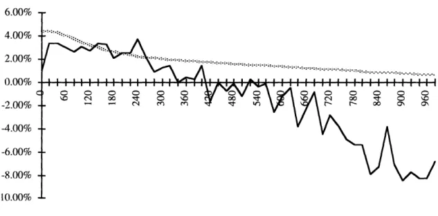
7.4 Limiting Triggering Distance ... 49
8.0 Triggers and Cache ...53
8.1 Cache in ME Framework ... 53
8.2 Experimental Results ... 54
9.0 In-Sentence Bigrams ...55
9.1 Selection of In-Sentence Bigrams ... ... 55
9.2 Experimental Results ... 56
10.0 Conclusions, Related W ork and Future Directions ... 59
10.1 Summary and Conclusions ... 59
10.2 Related Work ... 61
10.3 Future Directions ... 62
Acknowledgments
First and foremost, I would like to thank Salim Roukos at IBM's Thomas J. Watson Research Center and Ronald Rosenfeld at Carnegie Mellon University. The work presented here was conducted while I was a visitor at TJ Watson during the summer and fall of 1993 and it was an extension of my previous work on trigger language models done at TJ Watson the preceding summer. Salim was my supervisor and mentor throughout my stays at TJ Watson. Roni Rosenfeld and I worked together on my earlier trigger language model exploration at IBM. Without Roni, many of the implementation issues related to maximum entropy would have not been resolved as efficiently. I would also like to thank Peter Brown and Robert Mercer presently at Renaissance Technology and Stephen Della Pietra and Vincent Della Pietra presently at TJ Watson. Peter, Bob, Stephen, Vincent and Salim all jointly conceived and developed the maximum entropy framework for building statistical models at TJ Watson. Finally, I cannot forget Victor Zue, my thesis supervisor, who took time out of his busy schedule to offer his valuable input.
Raymond Lau
MIT, Cambridge, MA
May, 1994
1.0 Introduction and Background
1.1 Language Models
Language models predict the probability of a word's occurrence given information
about the context in which the word is expected to occur. Language models are useful in speech recognition, machine translation and natural language systems. For example, in a speech recognition system, we are given some acoustic evidence, a, and are asked to predict the spoken word, w, or a word sequence. A typical approach would be to choose w such that
Pr(w I a) is maximized over all possible w. Pr(w I a) may be rewritten using Bayes' rule as
Pr(wla) = Pr(alw) Pr(w) Here, Pr(a) does not depend on the word w so to find the word w
Pr(a)
which maximizes this expression, we need to maximize Pr(a I w) Pr(w) where Pr(a I w) is the probability that we receive the acoustic evidence a given that the word w was spoken and
Pr(w) is the a priori probability that the word w occurs. The language model's task is to
provide the probability distribution for Pr(w). Language models may also be used to prune the list of possible words which need to be considered by the speech recognition system by eliminating words with low probability. As another example, consider a natural language system. Language models may be used to correct improperly formed sentences by scoring alternative sequences of words.
Statistical language models provide this probability distribution based upon statistical evidence gathered from a large sample of training text. For example, a simple zero order model may recognize that the word "the" occurs much more frequently in English training text than any other word. A statistical language model can take advantage of this information when making its predictions.
i S
1.2 Trigram Statistical Language Model
A very successful statistical language model is the trigram language model (Bahl et al. [1]). In the trigram model, the probability of a word is predicted by constructing a Markov
model whose state is based on the previous two words. The transition probabilities for the
Markov model are estimated from a large sample of training text. For example, in a very simple trigram, the probability of a word, w, given the previous two words, w_1and w-2may
be given by:
c (w_2w_l w)
Pr(ww_lw_2
P I
) c(w- 2wl ) (EQ 1)2
)
-C(W
w_
1)
In reality, we do not have enough training text to see a large sampling of trigrams for any given bigram key, w_1and w-2. If we assigned all trigrams w_2w lw which we have never seen
in the training data the probability of zero, our model would have a very poor performance. Instead, we also include bigrams in our model to assist in cases where we have never seen the trigram. Because bigrams only involve two words instead of three, we will see a much larger sampling of bigrams than trigrams in the training data. Similarly, we also want to incorporate unigrams into our model. The question then is, how do we incorporate all three sources of information into one model? In the deleted interpolation trigram model, we linearly
interpolate the three probability distributions. The probability of a word, w, given the previous two words, w-1and w_2 is:
+
r2+
C (W_l W) C (W_2W_I W)Pr(wlw-lw- 2) = +2 N c(w 1 ) 3 C(W-2 ) (EQ2)
Here, N is the number of words in the training corpus, the c('s are the counts of occurrences in the training corpus. The X's are parameters optimized over some heldout text not seen during accumulation of the c('s. The idea here is that the heldout text approximates unseen
Adativ
Sttsia agug oeln
test data, on which our model will ultimately be measured, so it should provide good estimates for the smoothing parameters. We will refer primarily to this deleted interpolation trigram model as simply the trigram model. The model given in (EQ 2) has a natural interpretation as a hidden Markov model, which has three hidden states corresponding to the unigram, bigram
and trigram distributions for each context. The trigram model has been highly successful because it performs well and is simple to implement and train.
1.3 Measuring Language Model Performance: Perplexity
Ideally, we would like to measure a language model's performance by considering the decrease in error rate in the system in which the model is incorporated. However, this is often difficult to measure and is not invariant across different embodiments. A frequently used measure of a language model's performance is the perplexity (Bahl [1] et al., section IX) which is based on established information theoretic principles. Perplexity is defined as:
PP(T)
= 2H(P (T),P(T)) (EQ 3)where H(P(T),P(T)), the cross entropy of P(T) (the observed distribution of the text 1) with respect to P(T) (the model's predicted distribution of the text) is defined as:
H(P (T), P (T)
) = -P
(x)logP (x) (EQ 4)xET
Although lower perplexity does not necessarily result in lower error rate, there is a clear and definite correlation (Bahl et al. [1], section IX).
1.4 Beyond Trigrams: Adaptive Language Models
The trigram model is rather naive. Our natural intuition tells us the likelihood of a word's appearance depends on more than the previous two words. For example, we would reasonably expect that the context of the text has a large impact on the probability of a word's
appearance; if we were looking at a news story about the stock market, the probability of financial terms should be increased. Much of this information is not captured by the trigram model. Also, the trigram model is static in that it does not take into account the style or patterns of word usage in the source text. For example, in a speech recognition system, the speaker may use a very limited vocabulary, and yet the trigram model's estimates are based on a training corpus which may not match the speaker's more limited vocabulary. The trigram model is unable to adapt to the speaker's vocabulary and style, nor to topic information which
is contained in a document. l
An improvement upon trigram model was proposed in Kuhn and De Mori [15] and Jelinek et al. [13]. The cache model takes into account the relative dynamic frequencies of words in text seen so far and incorporates this information into the prediction by maintaining a cache of recently used words. This results in up to a 23% improvement in perplexity as reported in Jelinek et al. [13]. However, the manner in which the cache component was combined with the trigram component was a simplistic linear interpolation. In Della Pietra et al. [7], a more disciplined approach was pursued. The static trigram model was considered the initial probability distribution. The dynamic cache distribution was then imposed as a
constraint on the probability distribution. The final probability distribution was the one which satisfied the cache constraint while minimizing the Kullback-Leibler distance or
discrimination of information (Kullback [16]) from the initial trigram distribution.
Improvements of up to 28% in perplexity were reported, albeit on a very small test set of 321 words.
1. Strictly speaking, models which depend only upon a limited amount of information such as the current
ment or the current session are not truly adaptive in that they can be considered a function of the current
docu-ment or session. However, the term adaptive language modelling is frequently used to refer to such longer context models so we will continue to use the term here.
Adpie ttsiclLngaeMdeln
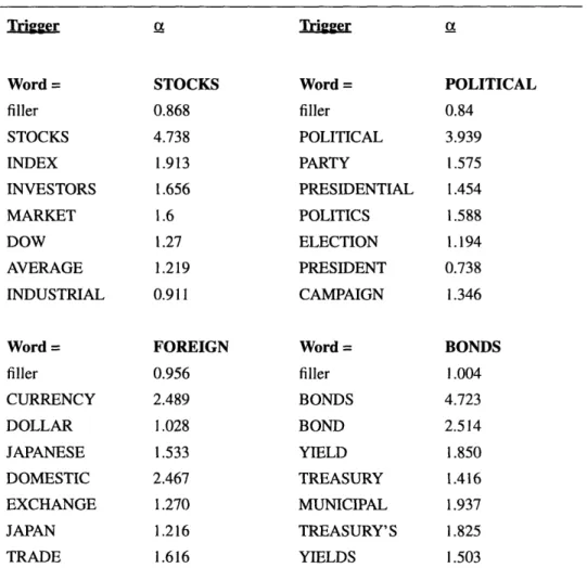
Another method in which the trigram model can be improved is to take triggers, or related words, into account. A trigger pair, A-B, is a sequence such that the appearance of A in the current document history significantly affects the probability of seeing B. Triggers in the document history may help establish the context of the current document. For example, in the
Wall Street Journal corpus the presence of the word "brokers" in a document makes the
appearance of the word "stock" approximately five times higher than normal. The additional presence of the word "investors' increases the probability of "stock" by another 53%. In earlier work by the author and others, initial attempts to model triggers were made and improvements of between 11% and 25% have been reported (Lau [17], Lau et al. [18], Lau et al. [19], Rosenfeld [21], Rosenfeld and Huang [22]).
A third approach to adaptive language modelling involves trying to identify the topic or domain of the current document and selecting an appropriately trained model for that topic or domain as opposed to relying on a general model trained on all topics and domains. Such an attempt was made at IBM (Roukos [23]). To identify the domain of a test document, the unigram distribution of the words seen so far is compared to the average unigram distributions of the domains in the training data. The attempt was somewhat successful when it came to decoding test documents from a domain which existed in the training data. However, in that attempt, widely disparate domains such as newspaper text and insurance documents were considered and the domains of the documents used for training were known in advance so there was no need to cluster documents into topics or domains through statistical means. Whether a similar attempt will be successful in modelling topics within a narrower domain such as the text of the Wall Street Journal and in situations where unsupervised clustering of documents into topics must be used will be investigated in the present work.
2.0 Experimental Preliminaries
2.1 The Wall Street Journal Corpus
For the present work, the text from the Wall Street Journal years 1987 through 1989 will be used as both the training and test copora. The Wall Street Journal task, perhaps because it is sponsored by ARPA, appears to be the one of primary interest within the adaptive
language modelling community2.Furthermore, the Wall Street Journal data made available by
ARPA includes both sentence and document boundaries, necessary for our model of
adaptation. We will consider a Wall Street Journal article to be the document we are dealing with. Articles tend to be on a narrow enough topic to benefit from an adaptive language model. We will use the data as processed by Doug Paul of MIT Lincoln Laboratories. We will use the non-verbalized punctuation version of the data along with the standard ARPA 20K vocabulary. By non-verbalized punctuation, we mean that text does not include punctuation,
such as periods and commas, as words. The text itself consists of roughly 39 million words. For the purposes of our experiments, we will separate the text into three corpora: a training corpus of 37 million words, a held-out corpus of one million words and a test corpus of 870 thousand words. The selection of the corpora will be chronological, that is, the earliest 37 MW will be used for the training corpus, etc. This results in a tougher test corpus than a random selection of documents for the corpora because topics in the text evolves over time and the topics in the test corpus may be substantially different from those in the earlier training and held-out corpora. However, we feel that this is the more realistic since our speech recognition
2. As a matter of fact, in the recent November '93 evaluation conducted by ARPA, language model adaptation was one of the specialized areas evaluated.
system, or whatever other system in which the language model will be used, will be confronted with data from the present and future, not from the past.
2.2 Adaptation Within a Document
We will use the document as the basic unit we are adapting to. That is, in our test environment, we consider the beginning of a document a clean slate and our goal is to improve the language model performance as we see more and more text of a document. This is not the sole possibility. An alternative might be to assume that each testing session proceeds in chronological order so that temporal relationships between documents may be exploited. The reason we made this choice is because the amount of data needed to statistically learn relationships across document boundaries is much greater. While our 37 million word training corpus has over 82 thousand documents, we will typically run our experiments with a much smaller subset of the training corpus consisting of five million words and roughly ten
thousand documents due to computational limitations. We do not feel that the smaller subset is sufficiently large to explore temporal relationships across document boundaries.
AdpieSttsia Lnug odlig1
3.0 Topic Specific Language Models
One possibility for building an adaptive statistical language model is to divide the documents into different topics and to have different models for each specific topic. Especially in the Wall Street Journal data, we would naturally expect dramatic differences between an article on politics and one on the equity markets. After having built topic specific models, we can then have one super-model which attempts to identify the specific topic of a document and uses the information provided by the topic specific models to make its
predictions. Since the trigram model has been quite successful, it would be natural to build different trigram models for each topic and then interpolate amongst them in some manner as to weigh the topic models according to the probability of the candidate document being a given topic. An added benefit of topic specific models is that they can be used as the basis for further adaptive extensions such as triggers. For example, a topic identification can be used to
select amongst various sets of triggers to consider for a given word.
3.1 Identifying a Suitable Set of Topics
Before we can build topic specific language models, we clarify exactly what we mean by "topics" and we must decide on how to arrive at a suitable set of topics. In some cases, such as in earlier experiments performed at IBM on building topic specific models (Roukos
[231), the documents are already tagged with topics selected by humans. In such a case, we can just use those topics as is, or perhaps clean them up slightly by consolidating small topics. Documents can then be clustered into the given topics (supervised clustering). However, the Wall Street Journal data which we have does not carry any topic information, so we must find some other way of clustering the documents into topics.
While it is possible to label the documents with topics by hand or to hand pick prototypes for each topic and perform a statistical clustering around those prototypes, we choose to follow a purely statistical approach of unsupervised (without human supervision) clustering. Our motivation here is that the success of statistical models such as the trigram model provides ample anecdotal evidence that statistical techniques may discover
phenomenon not evident to us humans.
3.1.1 Measuring the Closeness of Documents
In order to cluster our documents statistically, we need some measure of the closeness between two documents or perhaps between a document and a prototype. This measure does not have to be a true metric. It does not even have to be symmetric. However, it should reflect what we as humans consider as topic similarity. One possible measure is the cross entropy between the unigram probability distributions of two documents (or of a document and a prototype). However, preliminary attempts at using this measure met with poor results.
Another possible measure which proved effective in previous topic identification experiments (Roukos [23]) is the Kullback-Leibler distance between the unigram probability distributions of two documents (or of a document and a prototype). More specifically, let
D(A,B) represent the distance from document A to document or prototype B according to this
measure. Then:
D (A, B) =
log
(
N ( ) ) /(EQ
5)
wev A (cB(w))/NB
Here, cA(w) and CB(W) are the number of times w occurs in A and B respectively and NA and
NB are the number of words in A and B respectively and V is the vocabulary. Finally, log (0 / 0)
is defined to be 1. One of the problems with this measure is that if a word occurs in A and not in B or vice-versa, D(A,B) will be zero. To circumvent this problem, we smooth the
probabilities by adding a small factor which depends on the unigram probability of a word in the entire training corpus. Namely, instead of the- (, 'we will use we will use X + (l- )P (w). Here,+ - x) P . Here,
P,(w) is the unigram probability of w over all training data. Every word in our vocabulary occurs at least once in the total training corpus so this term is never zero. For A we select some convenient value such as 0.99. This smoothed measure is the one that we will use.
3.1.2 Clustering Documents
Once we have selected a distance measure, we still need to come up with an algorithm from clustering the documents into topics in an unsupervised manner. There are two basic approaches to this problem, namely top down and bottom up. For the purpose of generating approximately ten topics, a random sample of approximately 2000 documents should be adequate. An initial attempt at a bottom up approach which first compared all possible pairs of documents and a symmetrized variant of the final distance measure given in section 3. 1.1 took an excessive amount of computing time (over six hours on an IBM RS/6000 PowerServer 580, a 62 MIPS machine), forcing us to abandon such an approach. Instead, we will pursue a top-down approach.
We randomly select ten documents as the prototypes for the clusters. We then iteratively place each document into the cluster it was closest to until no documents change clusters. An issue which needs to be explored here is how to update the prototype of a cluster to reflect the addition of a new document or the removal of an existing document. One
possibility is to let the prototype's unigram distribution be the average unigram distribution of all the documents in the cluster. However, when we attempt this approach, we run into the following problem. Clusters with a large number of documents tend to have "smoother" unigram distributions. So, a few of the random seeds which are similar in their unigram distributions to a large number of documents became magnets, draw more and more
AdpieSttsia
Lnug odligl
documents into their clusters. In the end, we have only three extremely large topics. Examination of sample documents in these topics reveals no noticeable similarity of the documents within each topic. To alleviatethis problem, we instead choose a real document in a given cluster which is closest to the average unigram distribution for the cluster. Since the prototype for each cluster is a single representative document, each prototype is of equal "sharpness" and the aforementioned problem does not occur.
Running this procedure on 2000 documents randomly selected from our 5 MW test set converges in three iterations and results in eight clusters with more than a handful of
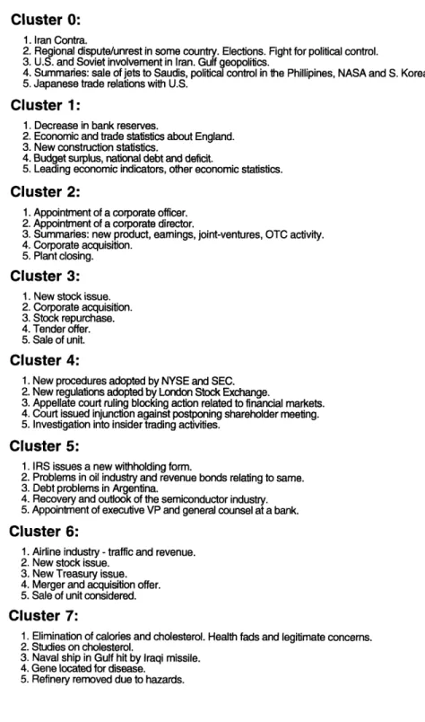
documents. (Two of the clusters have fewer than ten documents. The documents within them are folded into the other eight clusters using the same distance measure.) Five documents are randomly selected from each cluster and examined.We obtained a quick synopsis of the random documents for the clusters by randomly choosing five documents from each cluster and examining them. A summary of the five random documents selected from each cluster is given in Figure 1. The topics appear to successfully discern various financial topics such as economics in cluster one and rules and regulations in cluster four. However, non-financial subjects were not well separated by the topics obtained. Almost all non-financial documents were placed into cluster zero which ended up with 682 documents. Nevertheless, we feel that the clusters look good enough subjectively to be useful.
Cluster 0:
1. Iran Contra.
2. Regional dispute/unrest in some country. Elections. Fight for political control. 3. U.S. and Soviet involvement in Iran. Gulf geopolitics.
4. Summaries: sale of jets to Saudis, political control in the Phillipines, NASA and S. Korean developments. 5. Japanese trade relations with U.S.
Cluster 1:
1. Decrease in bank reserves.
2. Economic and trade statistics about England. 3. New construction statistics.
4. Budget surplus, national debt and deficit.
5. Leading economic indicators, other economic statistics.
Cluster 2:
1. Appointment of a corporate officer. 2. Appointment of a corporate director.
3. Summaries: new product, earnings, joint-ventures, OTC activity. 4. Corporate acquisition.
5. Plant closing.
Cluster 3:
1. New stock issue. 2. Corporate acquisition. 3. Stock repurchase. 4. Tender offer. 5. Sale of unit.
Cluster 4:
1. New procedures adopted by NYSE and SEC. 2. New regulations adopted by London Stock Exchange.
3. Appellate court ruling blocking action related to financial markets. 4. Court issued injunction against postponing shareholder meeting. 5. Investigation into insider trading activities.
Cluster 5:
1. IRS issues a new withholding form.
2. Problems in oil industry and revenue bonds relating to same. 3. Debt problems in Argentina.
4. Recovery and outlook of the semiconductor industry. 5. Appointment of executive VP and general counsel at a bank.
Cluster 6:
1. Airline industry - traffic and revenue. 2. New stock issue.
3. New Treasury issue. 4. Merger and acquisition offer. 5. Sale of unit considered.
Cluster 7:
1. Elimination of calories and cholesterol. Health fads and legitimate concerns. 2. Studies on cholesterol.
3. Naval ship in Gulf hit by Iraqi missile. 4. Gene located for disease.
5. Refinery removed due to hazards.
FIGURE 1. Synopsis of Five Random Documents in Each Cluster
Adaptiv
Sttsia Lnug odlig1
3.2 Topic Specific Trigram Models
The trigram model is a natural candidate for which we can build topic specific models and evaluate their performance on test data. If this effort proves successful, we can then add other information, such as triggers, to the topic specific trigram.
Once we have topic specific trigram models, there is still the issue of identifying which topic specific model or which combination of topic specific models to use when decoding test data. For an initial experiment, we can just tag each test document with its closest topic as determined by the distance measure used to create the topic clusters. This is more optimistic than a real decoding scenario because normally, we would not have the ability to "look ahead"
and access the entire document. We normally have access only to the document history as decoded so far. Any results obtained from this experiment will be admittedly an upper bound on the actual performance to be expected. Nevertheless, this experiment will help us to evaluate whether we should continue with the topic specific adaptation idea.
When we perform the experiment as described, we obtain perplexities which are even worse than using a single universal (non-topic specific) trigram model. One possible
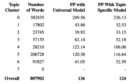
explanation might be because we do not have adequate data within each topic. So, instead, we can try smoothing the topic specific models with the universal model. We accomplish this by using linearly interpolating the topic specific model with the universal model using weights optimized over held-out data. The perplexity results of this experiment are shown in Table 1. The entire 37 MW training set was used to create the universal trigram model and the eight topic specific trigram models.
The topic specific trigram models appear to offer an improvement. However, it is worth noting that the least improvement occurs with the largest topics, namely topic zero and topic five. A possible explanation for this behavior is that documents without truly discerning
Adpie ttstclLagae oelig1
characteristics tend to be clustered together into larger topics so that models specific to such topics have little to offer given the non-uniqueness of the topics. Another possibility is that we may have just been unlucky with the construction of topics zero and five. However, when another experiment to further subdivide cluster zero into three topics is performed, we observe only a marginal improvement. (The overall perplexity using models for the subtopics
smoothed with the universal model is 228.83. This compares to the 236.13 shown in the Table 1 for topic zero.)
TABLE 1. Smoothed Topic Specific vs. Universal Trigram Model
Topic Number PP with PP With Topic
Cluster of Words Universal Model Specific Model
0 382435 249.56 236.13 1 17802 43.86 32.53 2 23745 39.92 33.15 3 57155 62.14 52.18 4 28210 122.14 106.06 5 206728 120.38 116.64 6 91827 41.05 32.59 7 0 Overall 807902 136 124
The upper bound on the improvement we can expect from the topic specific trigram models is from a perplexity of 136 to 124, only 8.8%. We do not feel that an 8.8%
improvement is enough to justify continuing with using topic specific models. Perhaps the topic selection algorithm can be improved but a related result arrived at by Martin Franz at IBM suggests otherwise (Franz [8]). Franz had Wall Street Journal data for years 1990 through 1992 obtained directly from Dow Jones, the publisher of the Wall Street Journal. Unlike the ARPA supplied data, his data set includes human derived subject classifications for each article. He built several trigram language models specific to a small number of subject classifications along with a universal model. Then, considering the most optimistic case, he took test documents for the subjects he had chosen and decoded them with the appropriate
interpolation of subject specific and universal language model. He reports an improvement in perplexity of around 10% only. This is not conclusive evidence that better statistically derived topics will not result in a much greater improvement. As already mentioned, what makes sense to a model need not make sense to humans at all, so human derived topics need not be considered sacrosanct. However, since the motivation behind building topic specific language models is because we feel that language properties are related to what we as humans would consider topics, the failure of Franz's experiment leaves us with little inspiration on making
further progress in this direction.
4.0 Maximum Entropy Models
All of the remaining models which we will discuss are maximum entropy models. An extensive theoretical derivation of a framework for statistical models based on the maximum entropy principle (Good [11]) can be found in Della Pietra and Della Pietra [5]. The author's prior efforts (Lau [17], Lau et al. [18] and Lau et al. [19]) also involves the creation of maximum entropy statistical language models. In this chapter, we recap the salient details of the maximum entropy framework.
4.1 Principle of Maximum Entropy
In a maximum entropy formulation, we are initially given some a priori information about the source being modelled. This information may be an existing model distribution or it may be the uniform distribution which corresponds to no prior information. We then define a series of linear constraint functions to present the information we wish to model. The principle of maximum entropy calls for a distribution which satisfies the linear constraint functions, hence capturing the information we are modelling, and which is "closest" to the initial distribution. Closest is defined in terms of Kullback-Leibler distance. Let Q be our initial distribution and Ybe the set of possible futures being predicted. Then the maximum entropy solution is the distribution P which satisfies the constraint functions and which minimizes the Kullback-Leibler distance D(P II Q):
D (P IIQ) = P (y) log Q ( ) (EQ 6)
yY (EQ6)
Adaptiv
Sttsia
Lnug odlig2
The name maximum entropy3 comes from the special case where Q is the uniform
distribution, hence, P is the distribution which satisfies the constraints and which maximizes the entropy function H(P):
H(P) = - P (y) logP (y) (EQ 7)
yE Y
The advantages of the maximum entropy approach include:
* It makes the least assumptions about the distribution being modelled other than those imposed by the constraints and given by the prior information.
* The framework is completely general in that almost any consistent piece of probabilistic information can be formulated into a constraint.
* The case of linear constraints, that is, constraints on the marginals, corresponds to no higher order interaction (Good [11]).
* If the constraints are consistent, that is there exists a probability function which satisfies them, then amongst all probability functions which satisfy the constraints, there is an unique maximum entropy one (Csiszir [2], Theorem 3.2 in particular and Della Pietra and Della Pietra [5]).
* The method of generalized iterative scaling4 (Darroch and Ratcliff [3]) provides an
iterative algorithm for finding the maximum entropy solution. Using this algorithm, we have the flexibility to add new constraints after the model has already partially converged provided that the new constraints are not inconsistent with the existing
ones and we can also remove existing constraints.
3. Where the prior distribution is not uniform, the maximum entropy solution is sometimes referred to in the lit-erature as minimum discriminant information, a technically more accurate name.
Fuzzy maximum entropy (Della Pietra and Della Pietra [5]) allows us to further "smooth" the maximum entropy distribution.
Some of the disadvantages of a maximum entropy approach include:
* There are no known bounds on the number of iterations required by generalized iterative scaling. Also, each iteration of generalized iterative scaling is
computationally expensive.
* Good-Turing discounting (Good [12]) may be useful in smoothing low count constraints (Katz [14]). However, it introduces inconsistencies so a unique maximum entropy solution may no longer exist and generalized iterative scaling may not converge.
4.2 Maximum Entropy Solution and Constraint Functions
If we let x denote the current history and y denote a future, in the maximum entropy approach the solution is of the form:
Xif (X, y)
Pr (x, y) = Q (x, y) e (EQ 8)
Here, Pr(x,y) is the desired maximum entropy probability distribution of (x, y), Q(x,y) is the prior or initial distribution, the i(x,y) are the constraintfunctions and the Ai are the model parameters or factors to be determined by generalized iterative scaling or gradient search. The
constraints themselves are expressed as:
Efi Pr (x, y) fi (x, y) = di (EQ 9)
x, y
In other words, we want the model expectation, EJf, to be equal to some desired expectation, di. The desired expectation may be set equal to the observed expectation, Efi, which can be
computed using the expression in (EQ 9), but with Pr(x,y) being replaced by the observed
AdpieSttsia
Lnug odlig2
probability, Pr(x,y). Note that the definition offi(x,y) is arbitrary. For concreteness, we cite an
example of a possible constraint function we may use in a language model. We can define a constraint function for trigrams as follows:
f1
if x ends in wlw2 and y = w3 (EQ 10) W~l~z~ 1W2-* W3 ) 0 otherwiseThus, in a maximum entropy model with such trigram constraints, we expect the model to predict w3when the history ends in wlw2with the same probability as observed during
training of the model parameters.
4.3 Maximum Likelihood Maximum Entropy
The maximum entropy model as stated so far gives a joint distribution of histories and futures. For our purposes, the word being predicted is the future and the document history is the history. What we really want is a conditional distribution on words given a history. The conditional probability is given by:
Pr(wlh) Pr(h, w) (EQ 11)
, Pr(h, w')
we VHere, V is the vocabulary and h is the current document history. As noted in Lau [17], this model is inadequate for most language modelling applications because we lack sufficient data to reliably estimate the event space of (h,w) pairs. More specifically, since we cannot
hope to observe more than an insignificant fraction of the possible O(IVlIh l) histories, we must
rely on a partition of the histories according to broad features. However, using such a
technique does not allow us to adequately rule out ridiculous histories such as a repetition of the word "the" 500 times. We cannot hope to come up with classifying features specific enough to rule out all such outrageous histories. Instead, we modify the model slightly in a
Adaptiv
Sttsia agae M
dlig2
manner suggested by colleagues at IBM. This modification was referred to as maximum likelihood maximum entropy in Lau [17] and we will continue to use that term here.
The definition of Efi in (EQ 9) can be rewritten as:
Ef i - Pr (h) XPr (wlh) fi (h, w) (EQ 12)
h w
Now, we will replace Pr(h)Q(h) with Pr(h), the observed probability of the histories in the training data:
Ef
iX
Pr(h)
XPr(wlh)
f i (h, w)
(EQ 13)
h w
This modification says that we are constraining the expectations to match the specific numerical values observed from the histories in the training data. Here, by definition, the probability distribution of the histories matches the observed training data distribution of histories as far as the constraint functions which are non-zero for a given history are
concerned. An interesting result of this modification is that the new model has the following equivalent interpretation:
Consider the exponential form of the model proposed by maximum entropy in (EQ 8) with our desired constraint functions. Now, find the set of factors, Xi, which maximize the likelihood of generating the data observed. This equivalence is the duality property shown in Della Pietra and Della Pietra [5] and derived constructively in Lau [17].
Finally, we note that (EQ 13) may be rewritten in a more useful form:
1TRd C jPr(wjh)fi(h,w ) (EQ14)
hE TR w
This equation is of practical importance. Here, TR denotes the training data. The summation over he TR means that we go through the positions, which correspond to the events (h,w), in the training data and accumulate the conditional expectations evaluated at each position. This
Adaptiv
Sttitia
Lagae oelig2
expression is particularly important because it allows us to practically evaluate the model expectations, Efi, without summing over all O(IV1lhl+l) possible history-word events! Many of
these histories never occur in the training data and this formulation makes it explicitly clear that we only need to consider those which do occur.
The other important equation, derived from (EQ 9), is the one defining how we can compute the desired expectations, which we are setting to be equal to the observed training data expectations:
di I TRI w) fi (h,w) (EQ 15)
(h, w) TR
4.4 Generalized Iterative Scaling
The method of generalized iterative scaling (Darroch and Ratcliff [3]) can be used to find the factors, Xi, of the model. Generalized iterative scaling is an iterative algorithm and is
guaranteed to converge to the correct solution, provided that the desired constraint
expectations are consistent. The GIS algorithm as applied to our model may be summarized as follows:
(i) Compute the desired expectations, di.
(ii) Initialize the factors, Xi, to some arbitrary initial value. (For con-creteness, we may consider them all to be initially zero.)
(iii) Compute the model expectations, Efi, using the current set of fac-tors.
(iv) Update the factors by:
(k+ 1) = i(k) + lnEfi (EQ 16)
Efi
Adpie ttstclLagae oelig2
(v) If not converged, go to (iii). (Convergence may be determined, for example, by the movement in the factors or by the change in per-plexity from the previous iteration.)
The GIS algorithm requires that for any event, (h,w), the constraint functions sum to one. When constraint functions do not naturally present themselves in such a manner, we can avoid the problem by artificially rescaling the constraint functions so that the sum to one requirement is met. To handle the varying number of constraints which may be active, we will
add afiller constraint for each future word5.
4.4.1 Computational Issues Involved with GIS
While the statement of the GIS algorithm itself is very simple and concise, many computational issues arise in creating a feasible and efficient implementation. Here we will
address generally the issues involved in implementing GIS for training maximum entropy language models. Lau [17] goes into quite some detail on describing the exact mechanics of implementing GIS for a trigger and n-gram language model.
The GIS algorithm can be broken down into three modules:
Initiator - The initiator sets up the files needed for the model and computes the
observed or desired values of the constraint functions.
Slave - The slave module is executed once per iteration. It computes the model expectations for the constraint functions given the current model factors. Since these model expectations are summed over the training data, we can divide the training data into segments and run multiple slaves in parallel, summing the results of all the slaves at the end of the iteration. This last step can be performed by the updater. This ability to parallelize the
5. Defining a different filler constraint for each word was suggested as a possible improvement over having one
execution of the slave is important because the bulk of the computation takes place in the slave since the slave must examine every event in the training set.
Updater - The updater takes the model expectations computed by the slave together with the desired expectations computed by the initiator and updates the model parameters. If parallel slaves were used, the updater also combines the results from the multiple slaves.
As already mentioned, most of the work is done in the slave where the model
expectations, Efi, defined in (EQ 14) must be updated for each event in the training data. If we examine the expression in (EQ 14), we note that potentially each active constraint's
expectation may need to be incremented for each event. By active constraint, we mean constraint's whose constraint function evaluates to a non-zero value for an event. This is potentially disastrous for constraints such as each word's filler constraint which are always active. However, because of the sum to one requirement for the constraints, we can compute the filler constraint analytically by subtraction at the end of the iteration. For some other constraints which are always active, such as unigram constraints if we choose to include them, we can circumvent the problem by observing that such constraints have a "default" value for most events. Hence we only need to explicitly accumulate over positions where the value is not the default value and analytically compute the correct value at the end of an iteration. A similar technique can be used to maintain the denominator in (EQ 11). (The expression
defined there is the model probability needed for computing the model expectations.) Namely, we consider the changes from one event to the next and add the changes into the denominator rather than explicitly recomputing the entire denominator. Note that the changes to the terms in the denominator correspond exactly to those constraints whose expectation needs to be updated from their default values so this leads to a convenient implementation.
AdpieSttsia
Lnug odlig2
4.4.2 Partial Updating of Constraints
Empirical evidence suggests that the model parameters (is) corresponding to
constraint functions (fis) with larger relative values converge more quickly to their final values under generalized iterative scaling. Lau [17] discusses a technique for emphasizing n-gram constraints to improve convergence rates for maximum entropy models with n-gram constraints. The idea is to rescale the constraint functions so that the most powerful
information, the n-gram constraints, have functions with a higher relative weight. Observing that eachfi is always used with the corresponding Xi, we can arbitrarily scalefj by a constant,
k, as long as we scale the corresponding Xi by 1/k. In our models with n-gram constraints, we
will want to make use of this technique to improve training convergence times. We can take this technique to the extreme and only update certain constraints during initial iterations. This corresponds to scaling the constraints we do not wish to update by a factor of zero so that they drop out. Frequently, we will want to make use of this technique and run the first few
iterations updating the n-gram constraints only.
5.0 Maximum Entropy Trigram Model
We mentioned that one of the advantages of a maximum entropy model is that we can combine information from various sources in the framework. Undoubtedly, given the success of the trigram model, we will want to include trigram constraints in at least some of the models we will investigate. In Lau [ 17], a maximum entropy trigram model achieved a perplexity of 185 on test data as compared to 170 achieved by a deleted interpolation trigram model. However, it was observed that the deleted interpolation model was an order of
magnitude larger since it included all unigrams, bigrams and trigrams whereas the maximum entropy model only included bigrams and trigrams with a count of three or more and unigrams with a count of two or more. The reason we did not try including more lower count constraints in the model was the prohibitive cost of computation involved.
In this chapter, we explore the maximum entropy trigram model once again. This time, we have switch to the more standardized ARPA 20K vocabulary with non-verbalized
punctuation. We will present a closed form solution to the maximum entropy trigram model, alleviating any computational bottlenecks. We will also examine improvements which allow the maximum entropy model to actually surpass the deleted interpolation model.
5.1 N-gram Constraints
To capture the trigram model's information within the maximum entropy framework, we use an n-gram constraint. First, let's define three sets:
S1 2 3 = { w1w2w3: count wlw 2w32 threshold }
S23 = { wlw2w3: w1w2w3 X S123 and count w2w3 > threshold
}
Adaptiv Statitica Langage odellng 3
S3= { wlw2w3: wlw2w3 q { S123 U S23 } and count w3 > threshold }
SO = { WW2w3: WW2W3 { S123 S2 3 U S3 } }
Then our constraint functionsf(h,w) will be indicator functions for the above sets with w = w3
and the last two words in h = wlw2. Several observations are worth making here. At any point, at most one constraint is active for a given future word because the sets are non-overlapping. This corresponds to the no-overlap formulation given in Lau [17]. The alternative is to define set S23 without regard to Sl23 and to define set S3 without regard to S23. One of the benefits of
this approach is that convergence of GIS is much faster for any model which includes the no-overlap form of n-gram constraints than the other form because there are fewer active
constraints active for any given event. Our experience with GIS shows that the fewer the number of active constraints, the faster the convergence rate. This was borne out in Lau [17] as far as n-gram constraints are concerned.
Another benefit is that in a model which includes only n-gram constraints, the no-overlap formulation gives us a model which can be computed in closed form so multiple iterations of GIS are not needed. To see this, consider the computation of the model
probability given in (EQ 11). For each event w1w2w3, we can express the model probability
as:
Xw w2w3
There active for any given event, so we only have one is at most one constraint Z( worry to There is at most one constraint active for any given event, so we only have one X to worry about. We should also recognize that since the denominator in (EQ 11) sums over all possible W3, it is a function of wlw2only. Now, if we further consider that there is one more equation,
namely that everything sums to one for a given wlw2then we observe that there are as many
equations as there are unknowns. (There is one equation for each w3 E V of the type given in (EQ 17) set equal to the observed training data expectation and the sum to one equation. There
Adativ SttstclLagae oelig3
is one unknown for each w3 E V, the Xs, and there is one Z(wlw2).) Thus, a closed form
solution exists.
5.2 Performance of ME N-gram Model
To evaluate the performance of our maximum entropy n-gram model, we construct a deleted interpolation trigram model out of the small 5 MW training set and evaluated its performance on our 870 KW test set as a baseline for further comparisons. This deleted interpolation model achieves a perplexity of 225.1. Next we construct two maximum entropy n-gram models with different cutoff thresholds for the definitions of the sets S12 3, S23 and S3. With a threshold of 3 for each set, our model achieves a perplexity of 253.5. With a threshold of two for each set, our model achieves a perplexity of 247.9. Franz and Roukos [9] reports that a threshold of one, which corresponds to all n-grams as in the deleted interpolation case, does not perform well. One possible reason for this is because of the unreliability of count one data and the strict constraints imposed by the maximum entropy framework based on this unreliable data. As a final comparison, we construct a deleted interpolation model which uses only unigram, bigram and trigram counts of at least three. This model achieves a perplexity of 262.7. Note that this final model has roughly the same amount of information as the maximum entropy model with a threshold of three. It seems that maximum entropy performs better than deleted interpolation when the two models are of roughly the same size. However, we cannot directly build a maximum entropy model with a threshold of one in order to capture the same amount of information as available in the full trigram model. Doing so would cause
performance to deteriorate significantly (Franz and Roukos [9]). Thus, we cannot match the full deleted interpolation model with the machinery we have developed so far. The results of the experiments involving the various N-gram models are summarized in Table 2:
TABLE 2. Deleted Interpolation vs. Maximum Entropy Trigram Model
Amount of
Model Information Perplexity
DI 3.5M 225.1
ME w/threshold of 2 790K 247.9 ME w/threshold of 3 476K 253.5
DI w/threshold of 3 790K 262.7
5.3 Improvement Through Smoothing
One possible way of incorporating the lower count trigram information in the
maximum entropy model is to first smooth the information. The favorable maximum entropy results reported in Lau et al. [18] actually included smoothing of the n-gram constraints. The exact improvement due to smoothing were never isolated and examined in that case.
Similarly, experimental evidence witnessed by colleagues at IBM in applying maximum entropy modelling to the problem of statistical machine translation suggests that smoothing may be very important (Della Pietra and Della Pietra [6]). In the following section, we pursue two approaches to smoothing the n-gram data.
5.4 Fuzzy Maximum Entropy with Quadratic Penalty
Della Pietra and Della Pietra [5] introduces a framework which they have dubbed
fuzzy maximum entropy. Fuzzy maximum entropy is a more generalized formulation of
maximum entropy where the constraints (EQ 9) are allowed to be relaxed. Strict equality is no longer demanded. Instead, as we deviate from a strict equality, we must pay a penalty. We no longer seek the solution which minimizes the Kullback-Leibler distance given in (EQ 6). Instead, we minimize the sum of the Kullback-Leibler distance and the penalty function, U(c).
We require that the penalty function be convex. The special case of an infinite well penalty function
Oifc. = d.
U(c) = i (EQ 18)
oo otherwise
corresponds to the standard maximum entropy setup. Here, an exact equality of the constraint expectation, ci, and the desired value, di, results in a zero penalty. Otherwise, we have an infinite penalty.
One way to think of the fuzzy maximum entropy framework in the context of smoothing is that we can make use of penalty functions which penalize deviations in more reliably observed constraints to a greater degree than deviations in less reliably observed constraints. Thus, we admit a solution where the less reliably observed constraints are relaxed in order to improve overall smoothness.
We consider the following quadratic penalty function:
U(c) = Ci -di) 6iJ (cj - dj) (EQ 19)
i, J
Here, we can think of c as the covariance matrix. Unfortunately, computation of is 6
nontrivial. As a matter of fact, we have to consider all possible pairs of constraints. Instead we will consider only the diagonal entries of c, that is, we will only consider the variance of each constraint.
An intuitive interpretation of the quadratic penalty function with a diagonal covariance matrix is the following. Instead of requiring a strict equality to the desired value, di, of a
constraint, we can think of a Gaussian distribution centered at the desired value. The width of the Gaussian is determined by the variance. The variance of the ith constraint function is given by aii =E(i 2)- (Efi) where as beforeE denotes the observed value summed over all events in
AdpieSttsia Lnug odlig3
the training data and N is the size of the training data. The constraints with a high number of observations would have a low variance and hence a smaller Gaussian.
In Della Pietra and Della Pietra [5], a variant of the generalized iterative scaling algorithm which can handle fuzzy maximum entropy is developed. For the case of a quadratic penalty with a diagonal covariance matrix, the update step in GIS is replaced with the
following at the end of iteration k:
Efik 1 (k +
1)
e Ef ci= Gii (EQ 20)
(k+ 1) (k+ 1)
xih ) = xi(k) +68X( (EQ 21)
(k + ) (k) (k+ 1)
Ci = C -_ (k Iii (EQ 22)
Initially, ci(O) = di. To solve (EQ 20) for the update value 8ki(k+ I), we must use a numerical root finding algorithm such as the Newton-Raphson method.
Some of the benefits of this approach to smoothing are:
* Smoothness here has a precise definition, namely, entropy. This definition is rather natural for the case of a perfectly smooth distribution, the uniform distribution, corresponds to that of maximum entropy.
* The generalized iterative scaling modified as described is guaranteed to converge. * There is very little additional computation required per iteration as compared to the
regular GIS algorithm. (However, we may need more iterations. Also, the special case of non-overlapping constraints such as the n-grams only case we are
considering can no longer be solved in closed form.)
A disadvantage is:
The choice of a penalty function is subjective. We have selected our particular function mainly on the basis of computational convenience although we feel that the selection is reasonable.
5.5 Good-Turing Discounting
Another possible approach to smoothing is to apply Good-Turing discounting to the desired constraint values, di. The use of Good-Turing discounting with the back-off trigram
model was discussed in Katz [14]. We use the same formulation here. Let r represent the "count" of a constraint, that is, r = di* N where N is the size of the training text. Note that r is
guaranteed to be an integer when we define the desired constraint values to be the observed values in the training data as given by (EQ 14). Then, the discounted count Dr is given by:
n
(r
1)
r+ nr (k + l)nk+ I r n Dr =(k- , for (1 < r<
k) (EQ 23) 1-nlHere, nidenotes the total number of constraints whose count equals i and k is the maximum count for which we are discounting. As in Katz [14], we will use k = 5 and we will omit all singleton constraints, that is, we will set D1= 0. Also, because we expect the constraint functions from sets S1 2 3, S23 and S3 (defined in section 5.1) to have varying reliability for a
given count, we will compute a set of discounted counts separately for each set. Some of the advantages of using Good-Turing discounting are:
It was successful with the back-off trigram model, which resembles our no-overlap n-gram constraint formulation somewhat.
It is computationally easy to implement, requiring only a minor adjustment to the GIS update step.
Some disadvantages of this method include:
* GIS is no longer guaranteed to converge since the discounted constraints imposed are no longer consistent with the observed training data. In reality, we expect that GIS will eventually diverge given discounted constraints.
* There is no easy way to apply discounting to overlapping constraints because we no longer have counts for partitions of the event space. However, even if we combine n-grams with other information in an overlapping manner, we can still discount just the n-gram constraints because those are non-overlapping with each other.
5.6 Results of Smoothing Experiments
We build two maximum entropy n-grams only language models using the fuzzy maximum entropy with quadratic penalty and Good-Turing discounting smoothing methods discussed. These models use the same training and test data used to build the unsmoothed maximum entropy n-grams only model and the deleted interpolation trigram model. For the quadratic penalty fuzzy maximum entropy model, we choose to include constraints with a count of two or greater only because the inclusion of count one constraints would be a serious computational bottleneck. The training perplexities after each iteration are given in Table 3. For the model with Good-Turing discounting, we will discount counts less than or equal to five and we will omit singletons to insure a fair comparison with the fuzzy maximum entropy experiment. The discounted counts for the sets S1 2 3, S2 3 and S3 are given in Table 4. Note that
both of these models have the same amount of information as the threshold of two maximum entropy n-grams only model examined in section 5.2. A comparison of the performance of the
smoothed models on test data is given in Table 5. As we can see, smoothing of the maximum entropy model certainly helps performance. Good-Turing discounting appears to be more helpful than fuzzy maximum entropy. As a matter of fact, the discounted maximum entropy model with thresholds of two on the constraints marginally outperformed the deleted interpolation model which includes singletons.
TABLE 3. Training Perplexities for Fuzzy ME N-grams Model
Iteration Perplexity 1 20010 2 105.1 3 103.5 4 103.1 5 102.9 6 102.9
TABLE 4. Discounted Counts for Good-Turing Discounting of ME N-grams Model
Disc. Count for Disc. Count for Disc. Count for
Count S1 2 3 S23 S3
2 0.975 1.204 1.852
3 1.942 2.143 2.715
4 2.884 3.190 3.926 5 3.817 4.074 4.722
TABLE 5. Performance of Smoothed ME N-grams Models
Model Size of Model Perplexity
Deleted Interpolation 3.5M 225.1
ME w/threshold of 2 790K 247.9
Fuzzy ME w/threshold of 2 790K 230.3
Good-Turing Discounted ME w/threshold of 2 790K 220.9
Adpie ttstclLagae oelig3
Adaptive Statistical Language Modelling6.0 Self-Triggers
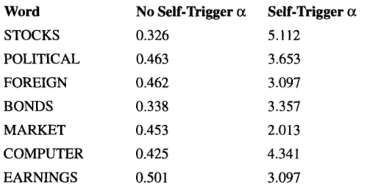
The success of the cache in Kuhn and De Mori [15] suggests that the appearance of a word has a substantial impact on the probability of a future appearance of the same word. Preliminary experimentation in Lau [17] and Lau et al. [18] reveal the same interesting phenomenon. We will refer to the effect of a word on its own future probability as the
self-triggering effect. In the present work, we will try to determine the improvement attributable to
self-triggers within a maximum entropy model.
6.1. Self-Trigger Constraints
For our experiment, we will only attempt to model whether a word has or has not already occurred in the current document. To do this, we introduce a self-trigger constraint for each word of the form:
f- (h, w) = (1 if w occurs in the document history h 0 otherwise
We include along with these self-trigger constraints the no-overlap n-gram constraints discussed earlier and a filler constraint for each word:
f w(h,w) = 1-f w (h,w) (EQ 25)
The purpose of the filler constraint is the following. Recall that GIS requires that all
constraints sum to one for each event. Without the filler constraint, the sum is either one if the self-trigger constraint function is zero, or two if the self-trigger constraint function is one. (There is exactly one n-grams constraint function which is one for a given event.) However,
with the filler constraint, the sum is always two so we can just mechanically scale by a factor of 1/2 to implement GIS.
6.2 Experimental Results
We train our maximum entropy model on our 5MW training corpus. For the n-gram constraints, we will only include constraints whose count is at least two and we will make use of the successful Good-Turing discounting technique here as well. For the self-trigger
constraints, we will likewise require a count of two. However, because most words occur more than once per document, almost all words (19K out of 20K) has corresponding
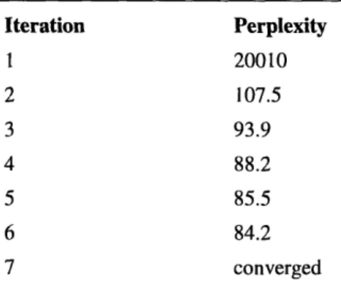
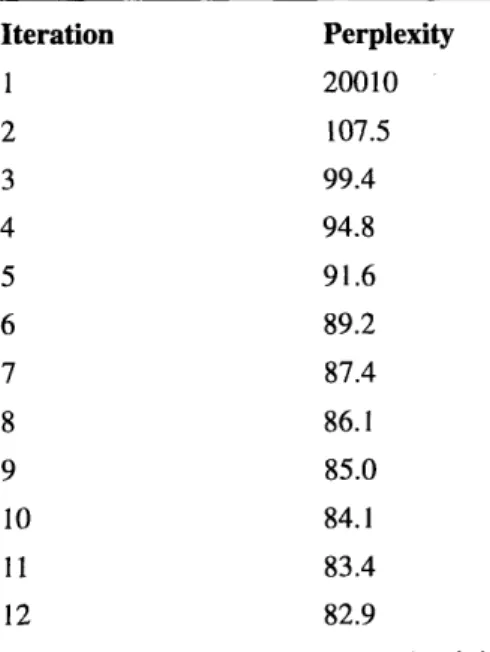
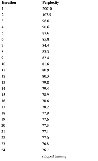
self-trigger constraints. To speed up the convergence rate, we will only update n-gram constraints on the first iteration as described in section 4.4.2. The training perplexities after each iteration are given in Table 6.
TABLE 6. Training Perplexities for Self-Trigger Experiment
Iteration Perplexity 1 20010 2 107.5 3 93.9 4 88.2 5 85.5 6 84.2 7 converged
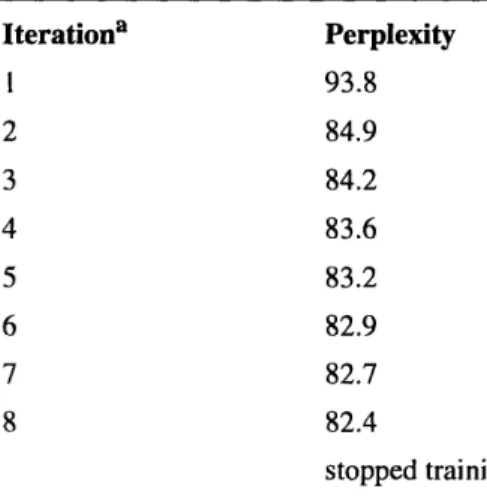
This model achieves a test set perplexity of 178.5, a 20.7% improvement over the deleted interpolation trigram model. The other worthwhile comparison is the deleted
interpolation trigram model combined with a dynamic cache similar to that of Kuhn and De Mori [15]. The dynamic cache makes a prediction based on the frequency of occurrence of the current unigram, bigram and trigram in the document history so far. It is combined with the deleted interpolation model through simple linear interpolation. Such a model has a perplexity