Automated Sub-Zoning of Water Distribution Systems
The MIT Faculty has made this article openly available. Please share
how this access benefits you. Your story matters.
Citation Sela Perelman, Lina et al. “Automated Sub-Zoning of Water
Distribution Systems.” Environmental Modelling & Software 65 (2015): 1–14.
As Published http://dx.doi.org/10.1016/j.envsoft.2014.11.025
Publisher Elsevier
Version Author's final manuscript
Citable link http://hdl.handle.net/1721.1/107418
Terms of Use Creative Commons Attribution-NonCommercial-NoDerivs License
Automated sub-zoning of water distribution systems
Lina Sela Perelman1, Michael Allen2, Ami Preis3, Mudasser Iqbal3, Andrew J. Whittle4
Abstract
Water distribution systems (WDS) are complex pipe networks with looped and branching topologies that often comprise of thousands to tens of thou-sands of links and nodes. This work presents a generic framework for im-proved analysis and management of WDS by partitioning the system into smaller (almost) independent sub-systems with balanced loads and minimal number of interconnection. This paper compares the performance of three classes of unsupervised learning algorithms from graph theory for practical sub-zoning of WDS: (1) Global clustering – a bottom-up algorithm for clus-tering n objects with respect to a similarity function, (2) Community struc-ture – a bottom-up algorithm based on network modularity property, which is a measure of the quality of network partition to clusters versus randomly generated graph with respect to the same nodal degree, and (3) Graph par-titioning – a flat parpar-titioning algorithm for dividing a network with n nodes into k clusters, such that the total weight of edges crossing between clusters is minimized and the loads of all the clusters are balanced. The algorithms are adapted to WDS to provide a practical decision support tool for water utilities. Visual qualitative and quantitative measures are proposed to eval-uate models’ performance. The proposed methods are applied and results are evaluated and compared for two large-scale water distribution systems serving heavily populated areas in Singapore.
Keywords: Water distribution systems; community structure; graph
1Postdoctoral Fellow, Department of Civil and Environmental Engineering, MIT,
Cam-bridge, MA, USA; email: [email protected] (corresponding author)
2Research Fellow, Faculty of Engineering and Computing, Coventry University, UK 3Postdoctoral Associate, Singapore-MIT Alliance for Research and Technology,
Singa-pore
4Edmund K. Turner Professor, Department of Civil and Environmental Engineering,
clustering and partitioning.
Graphical abstract
1. Introduction
The water sector worldwide is facing growing challenges in providing ad-equate quantities and quality of water to a continuously growing population. The finite water resources, climate change, and population grows and shift to warmer climates exercise an increasing impact on water resources and the water industry. To address this problem, various optimization-based formu-lations have been developed both at a regional and local scales. At regional scale, these include design and operation of water systems under future de-mand and water availability uncertainty (Chung et al., 2009; Housh et al., 2013), creation of new water resources by producing high quality water from saline or brackish water (Avni et al., 2013) and waste water reclamation (Zhang et al., 2013). At local scale, previous works focus on water distri-bution system design under demand (Babayan et al., 2005; Perelman et al.,
2013) and hydraulic model uncertainty (Fu and Kapelan, 2011; Laucelli et al., 2012), operation for leakage control (Giustolisi et al., 2008; Ulanicki et al., 2008; Price and Ostfeld, 2014), and reduction of potable water demand by on-site graywater reuse (Penn et al., 2013).
The creation of new water resources and re-use of waste water involve high economic costs and environmental impacts, hence, conservation of water through efficient end-use and active loss-control have attracted much interest both in research and practice (Mutikanga et al., 2013). Water conservation, traditionally, tends to focus largely on the end user, e.g. installing water efficient fixtures in the home and the workplace (Kunkel, 2003). Whereas, water utilities traditionally operate without consistent standards for water accounting and water loss control.
Water loss is the difference between the system input volume of water and all the authorized billed and unbilled (e.g. firefighting) water consumption (Kingdom et al., 2006). Water losses are characterized by real and apparent losses. Real losses are physical losses (e.g. leakages, bursts, tank overflows) that represent a waste of water resources. Apparent losses include meter inaccuracy, billing errors, and unauthorized use. Water losses, both real and apparent, constitute a major inefficiency in water supplies because water and energy resources are wasted, operating costs are increased, and water rev-enue is reduced. Water loss control requires a wide range of technologies supporting both re-active and pro-active approaches to reduce water losses including: (1) monitoring, (2) detection, (3) localization, (4) response, (5) pressure management, (6) leakage management, and (7) demand manage-ment.
Network sub-zoning is one of the tools for leakage and pressure man-agement for water loss control. The requirement of sub-zoning is to define the properties of the sub-zones within a network (e.g. size limit, total de-mand), to identify their boundaries (i.e. pipes or valves), and to monitor these boundaries for leakage and/or pressure control (with a limited number of meters). For example, the management of district metered areas (DMAs), has proven highly successful for leakage management (Thornton et al., 2008; Kunkel, 2003). A DMA of a water distribution system is a specifically de-fined area, in which the quantities of water entering and leaving the district are metered (Morrison, 2004). The subsequent analysis of flow calculates the level of leakage withing the district. According to Kunkel (2003) up to 85 % of the measured leakage in the UK has been eliminated through a national water loss control program based on DMA’s.
Recently, network sub-zoning has attracted many researchers with a vari-ety of applications. Zheng et al. (2013) and Zheng and Zecchin (2014) utilized network decomposition for an optimal design of water distribution systems. The full network is decomposed into sub-networks followed by a solution of a set of sub-problems representing each of the sub-networks using evolu-tionary algorithms. Perelman and Ostfeld (2011) and Deuerlein (2008) used graph decomposition methods to analyze network structure and connectiv-ity. Diao et al. (2014) used network decomposition method to accelerate the hydraulic simulation process by subdividing the network into smaller sub-networks and solving the hydraulic equations of each of the sub-sub-networks independently. Ulanicki et al. (2008) applied pressure management schemes to DMA by scheduling the set-point (output) pressures of boundary pressure relief valves which control the inlet pressures to the DMAs. Low operational pressures result in reduced leakage and minimization of the risk of bursts. Furnass et al. (2013) developed a data-driven methodology to identify cause-effect linkages of known water quality anomalies through mining the large volumes of water quality, hydraulic and asset data collected by water utility companies utilizing network internal partition having few inlets and outlets. This work focuses on network sub-zoning as a mitigation tool for water scarcity by facilitating water loss control. Urban water distribution systems (WDS) can reach a substantial size of hundreds to thousands of nodes (i.e. consumers) and links (i.e. pipes, valves). The layout of WDS is typically looped having multiple flow paths from the water sources to consumers. The looped layout of WDS, which provides a high level of reliability to the system supply in the event of mechanical failures (e.g. pipe breaks, valves malfunc-tions), imposes difficulties on water loss control. Due to the complexity of WDS, the re-design of an existing network can impair water supply, system reliability, and water quality (Grayman et al., 2009). A number of meth-ods for re-designing existing WDS into independent areas, by the closure of existing valves or disconnection of pipes, have been suggested. These vary from manual trial and error approaches, involving identification of wa-ter mains, manual division into districts, and hydraulic simulations (Murray et al., 2010), to highly sophisticated automated tools integrating network analysis, graph theory and optimization methods. The partition of the net-work is typically achieved by using graph algorithms, e.g. breadth first search and depth first search (Deuerlein, 2008; Perelman and Ostfeld, 2011; Ferrari et al., 2013; DiNardo et al., 2013a), multilevel partitioning (DiNardo et al., 2013b), community structure (Diao et al., 2013), and spectral approach
(Her-rera et al., 2010). The selection of pipes that need to be disconnected is found by iterative procedures (Ferrari et al., 2013; Diao et al., 2013) or genetic al-gorithms (DiNardo et al., 2013a,b).
Despite the recent developments, the application of proposed sub-zoning methods to real large-scale water distribution systems has been found to be generally limited (Mutikanga et al., 2013). Furthermore, there is a lack of consensual quantitative measures for evaluating system partition, hence the results are generally analyzed qualitatively.
This work presents: (1) a generic framework for simplifying the full-scale WDS by partitioning the system into smaller (within specified size limits), balanced sub-zones with minimum number of inter-connecting pipes/valves and (2) qualitative and quantitative measures for evaluating the performance of the network decomposition models. Three types of unsupervised learning algorithms are compared: global clustering – representing a more naive ap-proach given limited information about the WDS, community structure – adopted from social studies with similar previous application to WDS sub-zoning (Diao et al., 2013), and network partitioning – adopted from dis-tributed computed and previous similar application (DiNardo et al., 2013b). In graph theory, these algorithms aim at grouping similar or closely connected vertices such that the set of nodes in each group has better connections to the nodes belonging to the same group than to the remaining nodes in the network.
Following the position paper of Bennett et al. (2013) for characterizing the performance of environmental models, this paper is structured as follows: Section 2 introduces the graph theory methods; Section 3.2 defines visual and quantitative performance criteria; Section 4 demonstrates the methods and their performance using an illustrative example; Section 5 shows the applica-tion to two large-scale water distribuapplica-tion systems serving heavily populated areas in Singapore; Section 6 evaluates and compares the different methods based on the performance measures for sub-zoning; Section 7 summarizes current work and suggest direction for future research.
2. Methods
The application of the sub-zoning to WDS involves defining full network model based on the available data, formulating a decomposition method based on the network graph, evaluating the performance of the method based
on visual, qualitative and quantitative measures, and providing a practical decision support tool for water utilities.
Many of the processes in physical, cyber, and social systems are described by complex networks or graphs. The water distribution network can be natu-rally represented as a graph G = G(V, E) over a set of vertices (nodes) V and a set of connecting edges (links) E, where the vertices represent consumers, sources, and tanks and the edges – pipes, pumps, and valves. The graph can be characterized by nodal weights wi, i ∈ V (e.g. demand, elevation), link
weights wj, j ∈ E (e.g. diameter, flow), and an adjacency matrix A based
on network topology. The graph division to clusters is designated by the set C = (c1, . . . ci, . . . , ck) where each node i uniquely belongs to one of the
clusters i ∈ ck. In this work, we adopt and adapt popular approaches from
the three branches of graph theory to sub-zoning of WDS.
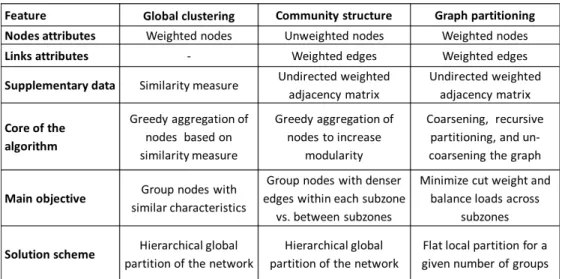
Clustering, community structure, and partitioning are closely related methods for understanding and analyzing complex systems, which have been extensively studied by a large interdisciplinary community over the past few years (Schaeffer, 2007; Fortunato, 2010). Generally, given a data set, the goal of these methods is to divide the data set into clusters such that the elements assigned to a particular cluster are similar or better connected in some predefined sense then to elements in other clusters. Global clustering is related to grouping sets of points which are close to each other, with re-spect to a measure of similarity defined for each pair of points. Community algorithms reveal the natural community structure using the concept of edge density, i.e. intra-clusters versus inter-cluster edges. Graph partitioning di-vides the graph into a predefined number of groups such that the number of inter-cluster edges is minimal. The methods differ by their required input, underlying objective, and output. The main features of the three classes of methods in graph-theory are summarized in Figure 1 and are described next.
2.1. Global clustering
Global clustering is one of the traditional algorithms for clustering n objects with respect to a similarity function (Hastie et al., 2009). It produces a multi-level or an hierarchical structure of the graph, where each level of the clustering hierarchy defines a different subset and each top-level cluster is composed of sub-clusters. A bottom-up hierarchical algorithm starts with each node forming a unique cluster, followed by a sequential grouping of the two most similar clusters and computation of the centroid of the newly
Figure 1: Comparison of algorithms considered for sub-zoning of WDS
formed cluster. This procedure is repeated until all nodes are grouped into a single cluster.
The basic similarity measure of nodes in a physical network is their ge-ographical position. In water distribution systems, distant nodes are not expected to be connected, hence the distance between a pair of nodes can be used as a measure of their similarity, i.e. similar nodes will be close to each other. Given two nodes u and v and their corresponding locations, (ux, uy)
and (vx, vy), the similarity between two nodes is computed as the Euclidean
distance:
d(u, v) = q
(ux− vx)2+ (uy − vy)2 (1)
and the mutual similarity measure between two clusters ci and cj is
com-puted as the average of the similarities of the nodes belonging to the clusters, as: D(ci, cj) = 1 |ci||cj| X u∈ci,v∈cj d(u, v) (2)
where |ci| is the size of cluster ci.
The main steps of the algorithm are described in 2.1.1 and full description can be found in Hastie et al. (2009).
2.1.1. Bottom-up hierarchical clustering algorithm main steps:
Given a graph with nodal weights wu (e.g. demands) and a dissimilarity
measure d(u, v)∀u, v ∈ V :
1. Start with each node as an individual cluster.
2. Compute the dissimilarity between all pairs of nodes (Eq. 1). 3. Find the least dissimilar pair and group them into one. 4. Compute dissimilarity between new clusters (Eq. 2). 5. Repeat steps 3 and 4 until one cluster remains.
In application to WDS, the number of clusters in which to group the nodes is not known priori, hence knowing the entire hierarchy of the network can be very informative. However, an additional procedure is required to decide how to partition the network. The attained hierarchical clustering of the graph is traversed in a top-down direction. The size (or load) of each top-level cluster is compared to a desired upper bound. If the size of the cluster does not satisfy the size constraint, the traverse continues to attain smaller sub-clusters. Additionally, since the Euclidean distance measure does not consider the connectivity of nodes, the intra and inter-connectivity of each cluster is verified. Finally, to satisfy lower bound constraint on cluster size, small connected clusters are grouped together. The main steps of the algorithm are summarized in 2.1.2:
2.1.2. Clustering algorithm for WDS sub-zoning main steps:
Given network graph G = (V, E), nodal weights wu, a dissimilarity
mea-sure d(u, v), and sub-zones upper limit size Wmax:
1. Attain the location of WDS nodes, i.e. ux and uy ∀u ∈ V .
2. Execute graph clustering algorithm 2.1.1 using the location of nodes. 3. Attain the hierarchical structure of the system G = (V, E, C) where
each level (cut level) of the clustering hierarchy defines a different sub-set.
4. Start at the top (all nodes belong to a single cluster), set cut level = 1, j = 1.
5. Compute the weight of each cluster:
Wci =
X
u∈ci
6. Check upper bound for each cluster ci: if Wci > W
maxupdate cut level =
cut level + 1 and continue to the next level; otherwise create new sub-zone zj = ci and update j = j + 1.
7. Repeat steps 5 and 6 until Wci ≤ W
max, for each cluster c
i ∈ C.
8. Check connectivity of each sub-zone zj using breadth first search
al-gorithm (Lee, 1961). Add disconnected nodes to a connected cluster based on adjacency matrix of the graph.
9. Check lower bound for each cluster zj: if Wzj < W
min group adjacent
clusters together based on the adjacency matrix A.
2.2. Community structure
Community structure is also a bottom-up hierarchical algorithm exploit-ing network modularity property as the quality measure of the partition. Modularity, a very popular (Fortunato, 2010) measure of the quality of net-work partition into clusters, was first introduced by Newman (2004). It is based on comparing the density of edges in the underlying division into sub-graphs to the density of edges if the graph was randomly divided into sub-graph with respect to the same nodal degree (i.e. number of incident edges). Since a random graph is not expected to have a cluster structure, a good community structure would have a higher modularity value. Modular-ity is always smaller than one, and can be negative as well. The theoretical value of modularity is defined as (Clauset et al., 2004):
Q(G, C) = 1 2m
X
ij
(Aij− Pij)δ(ci, cj) (4)
where m is the number of edges of the graph, A is the adjacency matrix, Aij
and Pij is the actual and the expected number of links between nodes i and
j, respectively, and δ(ci = cj) = 1, δ(ci 6= cj) = 0 indicating whether nodes
i and j belong to the same cluster c (i.e. Kronecker delta). The expected number of edges in a random graph between nodes i and j with respect to the same node degrees, ki and kj, respectively, is Pij = kikj/2m.
Practically the modularity can be computed as (Clauset et al., 2004):
Q(G, C) =X i∈C eii− X i∈C a2i (5)
where eii is the fraction of the number of intra-cluster edges and ai is the
The change in modularity can be computed according to:
∆Q(G, Cci,cj) = Q(G, C − ci− cj + ci∪ cj) − Q(G, C) (6)
A greedy algorithm (Newman, 2004) for maximizing modularity involves successive merging of two clusters that result in the highest increase in mod-ularity until all nodes are grouped into one cluster. The greedy algorithm was later revised to attain computational speed-up by using a more efficient data structures for updating of the modularity (Clauset et al., 2004). The main steps of the algorithm are listed in 2.2.1 and the full algorithm can be found in Newman (2004) and Clauset et al. (2004).
2.2.1. Community structure algorithm main steps:
Given a graph with weights on edges, i.e. G = G(V, E) and wj, j ∈ E:
1. Start with each node as an individual cluster.
2. Compute the change in modularity ∆Q resulting from merging every pair of clusters (Eq. 5-6).
3. Merge the pair with highest increase in modularity ∆Q. 4. Repeat steps 2 and 3 until one cluster remains.
As in global clustering, community structure method results in a hierar-chical clustering of the network. The exact partition of the graph is again selected by traversing the hierarchical structure from top to bottom and se-quentially checking the upper bounds of the created clusters. The procedure follows 2.1.2 exempt Step 8 since, in this method, only connected nodes can be joined together. This can be observed from Eq. 4, since nodes which are not connected can never contribute to modularity, i.e. δ(ci 6= cj) = 0. The
method can be simply extended to the case of weighted graphs, by replac-ing the degrees of the nodes with the correspondreplac-ing weights of graph links wj, j ∈ E. Similar application of the community structure approach to WDS
sub-zoning can be found in Diao et al. (2013). 2.3. Graph partitioning
The problem of graph partitioning consists of dividing n nodes of the graph into a predefined number k of roughly equal sized clusters such that the number of edges connecting the clusters is minimal and typically it is desired that the cluster have equal size. Graph partitioning is a fundamental approach used in parallel computing, for allocating tasks to multiple pro-cessors so as to minimize the communications and equally distribute the
computational burden among them. Many algorithms have been developed for the graph partitioning problem, mainly consisting of three classes of al-gorithms – spectral, geometric, and multi-level partitioning. Hendrickson and Leland (1993) showed that multi-level graph partitioning can provide better partitions than the spectral methods at lower computational cost for a variety of problems, e.g. finite element methods and linear programming. The graph partition problem was later extended and generalized Karypis and Kumar (1998) and is used in the current work for the partitioning of water distribution systems.
The graph partition problem is solved by performing a sequence of bisec-tions of the graph G = G(V, E), wi, ∀i ∈ V, wj, ∀j ∈ E. Initially, a 2-way
partition is obtained, then each cluster is further partitioned using 2-way partition. Finally, after a series of partitions, a k-way partition of the graph is attained. To attain a computationally efficient bisection of the graph, the graph is reduced by aggregating its nodes and edges, the smaller graph is partitioned, and the original graph is then recovered to construct the final partition of the original graph. The main step of the graph partition method are described in 2.3.1 and can be found in more detail in Karypis and Kumar (1998).
2.3.1. Graph partitioning algorithm main steps:
Given a graph with weights on nodes and edges, i.e. G = G(V, E), wi, i ∈ V , wj, j ∈ E, a multi-level partitioning involves:
1. Coarsening – the original graph G0is reduced into a sequence of smaller
graphs G1, . . . , Gmby aggregating its nodes and edges, such that |V0| >
. . . > |Vm|. The nodes are grouped based on heavy edge matching.
A matching Mi of a graph Gi is defined as a set of edges in which
no two edges are incident to the same vertex. The matching Mi is
detected by traversing the nodes of the graph and adding the highest weight link, incident to the node, to the matching set. This process is repeated until all nodes have been visited. The next coarser graph is constructed by aggregating the nodes connected by the edges in the matching set, i.e. Gi+1 = G(Vi+1, Ei+1) is induced by Mi. The weight
of the new aggregated meta-node in the coarser graph is equal to the sum of weights of the grouped nodes and the new set of edges equals to the union of the edges connecting the grouped nodes.
2. Partitioning – the reduced graph Gm is partitioned into two equal size
starting nodes using breadth first search and constantly updating the weight of the regions and the weights of the inter-connecting edges (edge-cut). The quality of the partition is sensitive to the selection of the initial nodes. To address this problem, ten nodes are randomly selected and ten different partitions are computed. The partition with the smallest edge-cut is selected as the initial partition. The parti-tion is then further refined by iteratively swapping a subset of vertices between the partitions that result in a smaller edge-cut. In each iter-ation, the gain of each node on the partition boundary, defined as the reduction of the edge-cut if the node is moved from one partition to the other, is computed, and the node with the largest gain is moved to the other part. The gains of all adjacent nodes are updated and the process is repeated by greedily selecting nodes with largest gain, until no improvement in the cut-edge can be achieved.
3. Recovering and refining – the original graph G0 is recovered from the
partition Cm. The recovery of the original graph can be attained simply
by going through the intermediate partitions Cm, Cm−1, . . . , C0 and at
each level i recover the partition of the original graph Gm, Gm−1, . . . , G0
by assigning the set of nodes grouped in each coarsening level i. During each recovery level, a local refinement heuristics is used to improve the partition Ci of the un-grouped graph Gi. This is achieved by swapping
vertices across the partition boundary to reduce the edge-cut similar to the refinement approach in the partitioning phase. Additionally, during the refinement the algorithm ensures that the balance constraints of the partition are not violated.
The graph partitioning algorithm results in a single partition of the WDS with balanced sub-zones connected by a minimal number of links between the sub-zones. The implementation of the partitioning algorithm to WDS requires the definition of network graph, weights for nodes and links of the graph, and the number of desired sub-zones. The number of sub-zones can be inferred from the desired size of the sub-zones. Similar application of this approach can be found in DiNardo et al. (2013b).
3. Performance evaluation
Evaluating the quality of a clustering algorithm or comparing different clustering methods is a difficult task. Mainly because the correct cluster-ing is unknown, clustercluster-ing algorithms rely on different data sets, and their
performance is dependent on parameter selection. Several qualitative and quantitative measures exist to evaluate the quality of the clustering (Scha-effer, 2007) that have been commonly used in the context of complex so-cial, biological, and information networks. For physical networks, measures evaluating the quality of the network partition are vaguely defined and less accepted. In this work several performance measures are proposed for evalu-ating and comparing the different network division methods and their affect on the end-user, i.e. water utility.
3.1. Visual performance analysis
Despite the power of quantitative comparisons, model acceptance and adoption, in the end, strongly depend on qualitative and often subjective considerations (Bennett et al., 2013). Hence, several visual qualitative per-formance measures are suggested in this work that provide a visual summary and an overview of the overall performance of the methods. Additionally, in the presence of multiple evaluation criteria visual measures allow a simple comparison of multiple methods without determining a strict formal holistic performance criteria in advance, as required in mathematical formulations. Particularly, the qualitative evaluation tools considered in this work are:
1. Adjacency matrix – visualization of the adjacency matrix is a graphical measure for evaluating the quality of the clustering. When the nodes of a graph are ordered randomly, there is no apparent structure in the adjacency matrix. Re-ordering of the nodes according to their clusters should reveal a tight block-diagonal structure of the adjacency matrix. The off-diagonal elements indicate clusters’ inter-connections. The desired outcome of a network division method is to minimize the appearance of the off-diagonal elements. This will be later linked to the worst and total cut-size quantitative measures of network division. 2. Aggregated network layout – the layout of the aggregated network re-sulted from the division of the detailed network, where each meta-node represents a sub-zone and the links represent the inter-connecting pipes and valves, provides a higher-level view of the network components and their interactions and can assist in the evaluation of the division of the network into sub-zones.
3. Kite-diagram – is used for multi-criteria evaluation. Each axis rep-resents a different performance measure standardized to a unit scale.
The results from these multi-criteria performance measures are com-bined into a set of kite-diagrams easily visually compared (van der Sluijs et al., 2005).
3.2. Quantitative performance measures
Multiple performance criteria are considered in the evaluation of network partition in light of the weaknesses of individual metrics. We adopt some of the common metrics from complex network analysis and adapt these metrics to the particular needs of the water network management.
1. Cluster size – is the weight of the cluster C, where weight is the pre-defined indicator of the network characteristic that the water utility would like to control. Examples for such indicators are number of con-nections, daily demand, or population. For better control of the WDS, it is typically desired that the weight of the sub-zones will be bal-anced (Grayman et al., 2009), enabling a more unified control actions at a system scale. Additionally, considering only network topology, i.e. number of nodes, could result in poor results, as in real network models the loads are generally aggregated to representative nodes and majority of network nodes represent cross-connections with zero demands. 2. Worst cut-size – cut-size is the number of edges that connect nodes in
cluster C to the rest of the nodes in the network V \C. The smaller the cut-size the better isolated the cluster. The worst cut-size is the maximum cut-size among all sub-zones. This measure affects the num-ber of flow meters that will need to be installed to monitor the flow in and out of the sub-zone. This measure also implies the number of field operation (valve closures) that will be required to isolate a individual sub-zone during routine or emergency response control. The goal is to minimize this number.
3. Total cut-size – is the summation of cut-sizes over all clusters, i.e. the total number of inter-connecting links. This number indicates the total number of pipes that need to be monitored for water loss control i.e. defining the number (and cost) of meters to be installed in the network. Naturally, this number grows with the number of desired sub-zones and should be minimized.
4. Recurrence of inter-cluster edges (RICE) – is the number of times that a unique link connected different clusters for different levels of parti-tioning. For example, if the network was divided into 5, 10, and 15
sub-zones, and a unique link appeared in all three partitions then its RICE is equal to three, if another link appeared only once then its RICE is equal to one. This measure can be used to evaluate the suitability of the clustering for a long-term flexible design versus here-and-now design. Initially, smaller number of flow meters can be installed in the network, resulting in a low level partition monitoring large sub-zones. In the future, the initial partition can be refined by installing additional meters monitoring smaller sub-zones utilizing the flow meters in place. 5. Running times – algorithms running times can also be considered in the evaluation of its performance especially if it should be executed in real-time mode. For off-line analysis running time is less compelling performance criteria.
4. Illustrative example
To demonstrate the methods and the performance analysis we introduce an illustrative example adopted from Alperovits and Shamir (1977). The network consists of six nodes connected by seven pipes arranged in two-loops. This benchmark network has been previously extensively studied for optimal design. Its layout and data is given in the supporting information (SI).
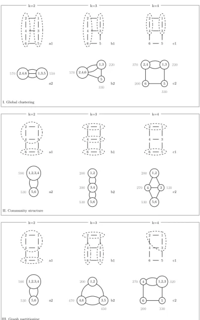
The illustrative network was partitioned into three different clustering lev-els, k = {2, 3, 4} sub-zones using the three methods: global clustering (GC), community structure (CS), and graph partitioning (GP). Figure 2 visually demonstrates the application of the three methods for three clustering levels. Figures 2 a1, b1, and c1 show grouped network nodes for each method and clustering level, Figures 2 a2, b2, and c2 show the resulting aggregated net-work structure and the size of each aggregated sub-zone in terms of demand. For example, Figure 2.I.a1 demonstrates network division into two clusters and Figure 2.I.a2 visualizes the corresponding aggregated network structure comprised of two sub-zones. Figures 2.I.b1-c2 show similar information for a finer division of the network into three and four sub-zones, respectively.
Table 1 subsequently lists the quantitative performance measures that can be inferred from Figure 2. For example, observing Figure 2.I.b2 network partition to 3 sub-zones where the size of sub-zones varies from 1 to 3 in terms of number of nodes and from 220 to 570 [daym3] in terms of daily demand. The worst cut-size is the maximum number of inter-connecting edges in the
aggregated network for an individual sub-zone. In this case the worst cut-size is equal to max{3, 3, 2} = 3. The total cut-size indicates the total number of inter-connecting edges in the aggregated graph and is equal to (3 + 3 + 2)/2 = 4. The number of repeating inter-cluster edges indicates the number of edges that appear more than once in all of the partitions. For example, edges connecting nodes 1-2, 3-4, 5-6 appear in all three partition levels. Additionally, GC and CS are multi-level methods in the sense that each top-level cluster is comprised of sub-clusters. For example, Figures 2.I.a1-c1, cluster {2, 4, 6} is comprised of smaller sub-clusters {2, 4}, {6} and cluster {1, 3, 5} – of sub-clusters {1, 3}, {5}. Hence, it is expected that the number of repeating inter-cluster edges will be higher for the hierarchical methods.
Table 1: Illustrative example
Method GC CS GP # Sub-zones 2 3 4 2 3 4 2 3 4 Max #nodes 3 3 2 4 2 2 4 2 3 Min #nodes 3 1 1 2 2 1 2 2 1 Max Demand 570 570 370 590 530 530 590 470 330 Min Demand 550 220 200 530 200 120 530 200 200 Worst cut-size 3 3 3 2 4 3 2 3 3 Total cut-size 3 4 5 2 4 5 2 4 5 Repeating edges 3 4 4 2 4 4 2 3 4
The results in Table 1 and Figure 2 demonstrate the different behavior of the methods even for such small network. Next, we apply the graph methods to real large-scale water distribution systems and evaluate and compare the quality of the sub-zoning.
5. Results 5.1. Application
This work was conducted in extension of the Wireless Water Sentinel in Singapore (WaterWise@SG) (Allen et al., 2011) and in collaboration with Singapores Public Utility Board (PUB). Singapore’s urban water distribu-tion system is highly complex due to densely populated areas. The suggested
III. Graph partitioning 1 2 3 4 5 6 a1 k=2 1,2,3,4 5,6 a2 590 530 1 2 3 4 5 6 b1 k=3 1,2 4,6 3,5 b2 200 470 450 1 2 3 4 5 6 c1 k=4 1,2,3 4 5 6 c2 320 270 330 200 II. Community structure
1 2 3 4 5 6 k=2 a1 1,2,3,4 5,6 a2 590 530 1 2 3 4 5 6 b1 k=3 1,2 3,4 5,6 b2 200 390 530 1 2 3 4 5 6 c1 k=4 1,2 3 4 5,6 c2 200 120 270 530 I. Global clustering 1 2 3 4 5 6 k=2 a1 2,4,6 1,3,5 a2 570 550 1 2 3 4 5 6 k=3 b1 1,3 5 2,4,6 b2 220 330 570 1 2 3 4 5 6 k=4 c1 2,4 1,3 6 5 c2 370 200 330 220
Figure 2: Illustrative example
methods have been applied to several water distribution networks serving dif-ferent districts of Singapore. The results for two of the districts are
demon-Table 2: Key physical characteristics of Network 1 & 2 Parameter Network1 Network2
# Nodes 2440 19402 # Reservoirs 1 2 # Tanks 1 2 # Pipes 1932 15622 # Valves 592 4476 # Pumps 6 2 Population 111,740 593,800 Demand [103m3/day] 16.98 92.06 Total pipe length [km] 41.046 341.26 Density [103km/km2] 2.565 5.687
strated in this work. Similar performance was observed when applied to all water districts. The data for the two networks is given in Table 2. For security reasons, the exact system layouts are not provided.
The application of the methods involves:
Input: The required input is network topology, geographic coordinates, weights of nodes and links. This information can also be read directly from a .inp network file (USEPA, 2002). Graph adjacency matrix, nodes and links weights are derived from the data listed in the input file. In current implementation, the weights for all links (i.e. pipes and valves) were uniform and nodal daily demands were set as nodal weights. Future applications will consider including weighted links.
Partition criteria: The features of the program allow the user to set sub-zone size constraints or the number of sub-sub-zones. Six different levels of net-work partition were tested in this net-work, particularly k = 5, 10, 15, 25, 35, 50, which corresponds sub-zone size of {20, 10, 8, 4, 3, 2}% of the total daily de-mand.
Method selection: The three algorithms for WDS sub-zoning were inte-grated in a python environment, with the following open source programming toolkit: (1) Global clustering – the hierarchical clustering algorithm was im-plemented in R (R Development Core Team, 2008) using agnes function part of the cluster package (Maechler et al., 2014) with Euclidean distance and av-erage linkage. The geographical location data, i.e. (xi, yi), ∀i ∈ V were used
Com-munity structure – the comCom-munity structure algorithm was implemented in R (R Development Core Team, 2008) using the fastgreedy.community (Clauset et al., 2004) part of the igraph package (Csardi and Nepusz, 2006). (3) Graph partitioning – the graph partitioning algorithm was implemented using the gpmetis function, METIS (METIS, 2013).
Performance evaluation: The quality of WDS sub-zoning is evaluated and the methods are compared based on the visual and quantitative performance measures previously presented.
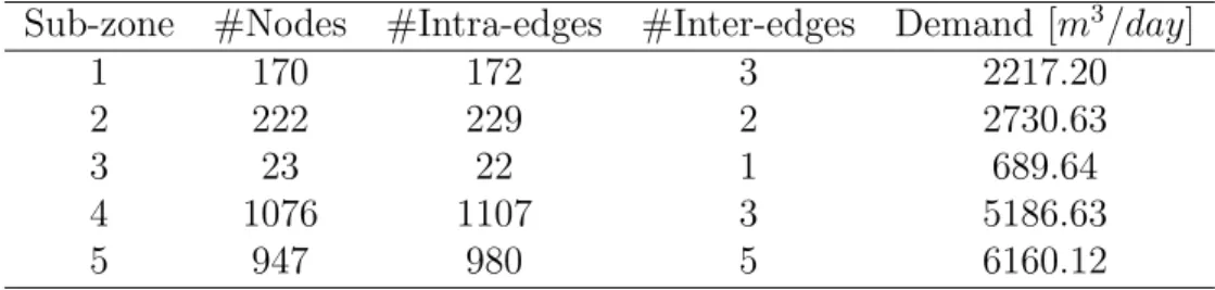
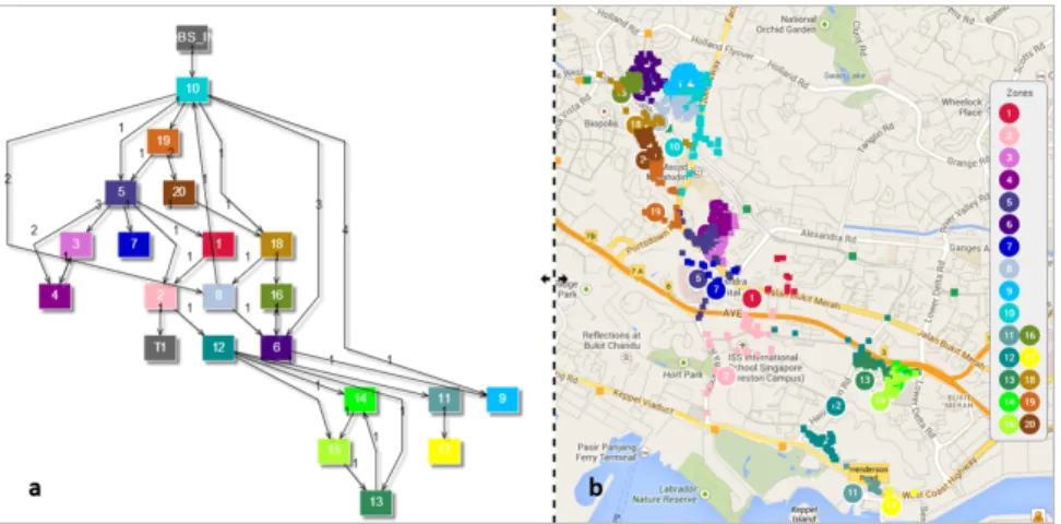
Final outcome: The final outcome of this work resulted in a web-based tool accessed by the authorized PUB operators, that enables choosing the desired number of sub-zones or, alternately, the size of the sub-zones, for a selected water distribution network. The output provides a summary of the network partition to sub-zones including the number of nodes, number of intra and inter cluster edges, and the daily demand; and an interactive map demonstrating classification of network nodes (using colormap) to sub-zones showing their inter-connecting links and a supporting aggregated network layout. An example of an output for Network1 using GP algorithm for k = 5 sub-zones is shown in Table 3. Figure 3 graphically shows the partition of the network to 20 sub-zones aggregated network layout (a) and map view (b).
Table 3: Graph partitioning results for Network 1 with 5 sub-zones Sub-zone #Nodes #Intra-edges #Inter-edges Demand [m3/day]
1 170 172 3 2217.20 2 222 229 2 2730.63 3 23 22 1 689.64 4 1076 1107 3 5186.63 5 947 980 5 6160.12 5.2. Network 1
This section compares and evaluates the performance of the three algo-rithms for Network 1. To get the initial value of the overall performance of the sub-zoning and its effect on the network we observe the structure of the adjacency matrix before and after sub-zoning. Figure 4 shows the adjacency matrices for Network1 – (a) original network and (b) clustering to k = 15 sub-zones using the GP algorithm. The columns and rows of the matrix are
Figure 3: Graph partitioning results for Network 1 with 20 sub-zones: (a) Aggregated network layout, (b) Map view
reordered corresponding to the sub-zones represented by the blocks of the matrix. A clear cluster structure of the network can be observed from Figure 4(b) compared to the original structure Figure 4(a).
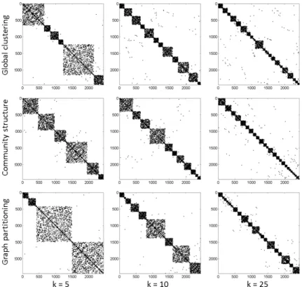
Figure 5 further shows the adjacency matrices for k = 5, 10, 25 sub-zones using the three methods – GC, CS, and GP. A clear cluster structure is evident from these figures, however, a practical comparison between the three techniques cannot be drawn. It is important to note, that the matrix blocks represent the size of the clusters in term of number of nodes and do not represent the demand of each cluster, since the adjacency matrix represents the connectivity between the nodes and does not depict the weights of the nodes. This stresses the need to consider the size of the sub-zones in terms of e.g. demands and not number of nodes in the graph. This claim is supported by Figure 2 in the SI showing the quantile plot of the distribution of demand versus the number of nodes in the sub-zones for k = 25 using GP approach. Additional outcome from the partition of WDS to sub-zones is the ag-gregated network layout. Figure 6 demonstrates the structure of Network 1 after partition to 25 (a) and 50 (b) sub-zones, based on the GP method, and the connections between the different zones and the network sources. The number on the edges shows the number of inter-cluster connecting links and the direction shows the direction of flow for a representative daily flow pattern.
Figure 7 demonstrates the performance of the three algorithms: global clustering (blue), community structure (red), and graph partitioning (black),
Figure 4: Adjacency matrix for Network1: (a) Original network, (b) Network divided into k = 15 sub-zones based on GP algorithm.
Figure 5: Adjacency matrix for Network1 divided into k = 5, 10, 25 sub-zones using GC, CS, and GP methods.
for k = 5, 10, 15, 25, 35, 50 on four suggested quantitative measures (Section 3.2): (a) total cut-size , (b) worst case cut-size, (c) cluster size, and (d)
recur-Figure 6: Aggregated network structure for Network1 based on GP: (a) 25 sub-zones and (b) 50 sub-zones
rence of inter-cluster edges. From the results it can be seen, that, as expected, the total number of inter-cluster connecting links grows with the number of sub-zones (Figure 7(a)). The maximum number of inter-cluster connecting links for a single sub-zone varies around 11, 10, and 9, for the GC, CS, and GP methods, respectively (Figure 7(b)). As the number of sub-zones grows, the demand load of each sub-zone decreases (Figure 7(c)). Figure 7(d) shows the fraction of inter-cluster edges that appear more than once during differ-ent sub-zoning levels. For example, approximately 16 % of all inter-cluster edges appeared more than once in divisions to k = 5, 10, 15, 25, 35 sub-zones based on clustering and community structure approaches. The recurrence of inter-cluster connecting edges is similar and higher for the hierarchical methods, i.e. clustering and community structure, compared to the flat par-titioning approach. This behavior remains similar for all the partitions (i.e. for k = 5 − 50 sub-zones).
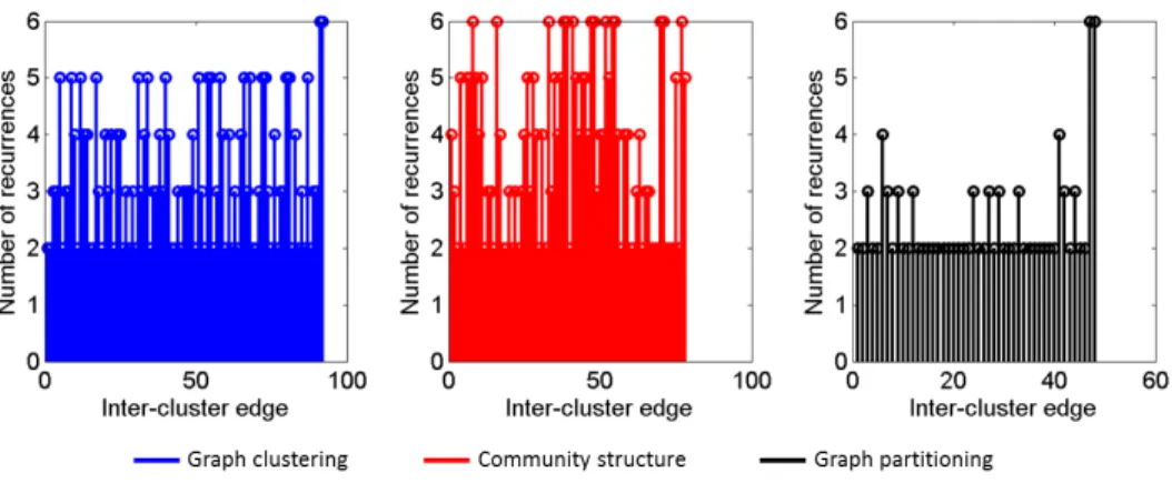
Figure 8 further shows the distribution of the repeating inter-cluster links (Figure 7(d)) for the three methods and six partitions. For each inter-cluster edge (x-axis), the plot (y-axis) shows the number of times that the edge appeared in all divisions, with six being the highest possible value corre-sponding to the number division computed. It can be seen that community structure method has the highest number of high frequency links (i.e. that
Figure 7: Quality measures for Network 1: (a) Total cut-size, (b) Worst case cut-size, (c) Sub-zone demand, and (d) Recurrence of inter-cluster edges based on GC (blue), CS (red), and GP (black)
appeared in most divisions), followed by the global clustering approach with similar distribution, whereas in the graph partitioning approach the majority of inter-cluster edges appear at most twice in all sub-zones.
5.3. Network 2
The performance of the three algorithms was next evaluated for the much more complex Network 2 (Table 2) using same performance measures. The tested methods exhibit similar performance when applied to Network 2. The qualitative performance evaluation measures for Network 2 are shown in Fig-ures 2-5 in the SI, including aggregated network structure, quantile
distribu-Figure 8: Recurrence of inter-cluster edges distribution for Network 1– GP (blue), CS structure (red), and GP (black).
tion plot of demand versus number of nodes, aggregated network structure, and distribution of repeating edges.
Figure 3 in SI shows the adjacency matrix before and after network par-tition to k = 50 sub-zones using GP algorithm. Demand distribution versus node distribution is shown in Figure 4 in SI for k = 50 using GP, demonstrat-ing that the size and the demand of sub-zones follows the same distribution for small sub-zones ( < 2.5 · 103[m3/day]). For larger sub-zones the size of the sub-zone is not correlated to its daily demand. Figure 5 in SI shows the aggregated network layout for k = 5 (a) and k = 50 (b) sub-zones using GP algorithm. Finally, Figure 6 in SI shows the frequency of the repeating inter-cluster links for the three methods and six partitions. Again, with the community structure method exhibiting the larger number of frequent links, followed by the cluster structure, while in the graph partitioning method most edges appear only twice.
The quantitative measures are shown in Figure 9. The results exhibit similar behavior to the previous application for Network 1. The total cut-size grows with the number of sub-zones (Figure 9(a)). The worst case cut-size for for a partition to 50 sub-zones varies around 37, 25, and 22, for the GC, CS, and GP methods, respectively (Figure 9(b)). The demand load of each sub-zone decreases as the number of sub-sub-zones increases (Figure 9(c)). Again, the frequency of repeated inter-cluster connecting edges is similar and higher for the hierarchical methods compared to the flat partitioning approach. This
behavior remains similar for all the partitions, k = 5, 10, 15, 25, 35, 50.
Figure 9: Quality measures for Network 2: (a) Total cut-size, (b) Worst case cut-size, (c) Sub-zone demand, and (4) Recurrence of inter-cluster edges based on GC (blue), CS (red), and GP (black)
The running times (Intel Core i7 2.9GHz 8GB of RAM) of the three meth-ods and six partitions for both networks are shown in Table 4. The graph partitioning approach is the most computationally efficient method, followed by the community structure and global clustering methods. The running times for the hierarchical methods increase with the increase of the number of sub-zones. Running times for the hierarchical methods depend primarily on the depth of hierarchical tree structure that needs to be traversed dur-ing the formation of the clusters, i.e. the number of cuts that need to be performed (Section 2.1.2). For the flat method, the changes in the running
times for Network 1, are not significant due to the relatively small size of the network. For Network 2, the running times decrease with the increase of the number of sub-zones. For smaller number of sub-zones, i.e. larger clusters, the graph partition algorithm spends more time on recovering and refining (Section 2.3.1) of the network as there are more intermediate par-titioning levels. Additionally, the running times of the algorithms depend on the cluster-size constraint or the number of sub-zones, and the weights associated with network nodes and links.
Table 4: Running times [mm:ss.ms] Network 1 Method # sub-zones Graph clustering Community structure Graph partitioning 5 00:01.1 00:00.5 00:00.2 10 00:03.9 00:02.1 00:00.2 15 00:06.3 00:05.2 00:00.2 25 00:12.4 00:07.2 00:00.2 35 00:22.7 00:16.8 00:00.2 50 00:27.7 00:21.8 00:00.2 Network 2 # sub-zones Graph clustering Community structure Graph partitioning 5 12:21.9 07:53.3 00:05.5 10 12:20.7 08:03.8 00:03.9 15 12:20.3 08:05.1 00:03.4 25 13:27.2 08:22.9 00:02.0 35 22:14.0 10:58.8 00:01.8 50 24:12.4 15:27.8 00:01.6
Finally, multi-criteria evaluation of the proposed methods can be visual-ized in an ensemble of kite-diagrams shown in Figures 10 and 11 for Networks 1 and 2, respectively, where each axis represents a different performance mea-sure standardized to a unit scale: (a) Worst cut-size, (b) Total cut-size, (c) Cluster size, (d) Recurrence of inter-cluster edges, and (e) Running times. This multi-criteria visualization allows for a relatively simple comparison of the methods for all partitioning for both networks.
Figure 10: Kite-diagram for Network1: (a) Worst cut-size, (b) Total cut-size, (c) Cluster size, (d) Recurrence of inter-cluster edges, and (e) Running times.
6. Discussion
The results presented in Section 5 demonstrate the applicability of three classes of clustering methods to sub-zoning of large-scale water distribution systems. The results demonstrate that, as expected, community structure and graph partitioning methods are superior to the simpler clustering ap-proach based on dissimilarity measure, since the former, rely on the infor-mation of connectivity between the nodes, whereas the latter requires only the location of the nodes. The community structure and graph partitioning can also assign weights to the links of the system. For example, the weights of the links can represent the diameters, flow, or head loss of the pipes and can be taken into account during the partition of the network. For example, if the sensor cannot be physically installed on small diameter pipes, then these pipes could be assigned a higher weight such that they do not appear as inter-connecting links. If the design objective is to segment the network by using existing valves, the weights of the links can be used to limit pipe closure to existing valves.
Figure 11: Kite-diagram for Network2: (a) Worst cut-size, (b) Total cut-size, (c) Cluster size, (d) Recurrence of inter-cluster edges, and (e) Running times.
methods applied to the two water distribution networks. A better perfor-mance would be to minimize four out of the five metrics, i.e. (a) Worst cut-size, (b) Total cut-size, (c) Cluster size, and (e) Running times. The last metric, i.e. (d) Recurrence of inter-cluster edges, should generally be maximized.
In terms of total and worst case cut-size (i.e. number of inter-cluster connecting links), the graph partitioning method generally outperforms the clustering and the community structure methods for Networks 1 and 2. This can be explained as the GP algorithm directly tries to minimize the cut-size, the CS algorithm greedily groups nodes to maximize network modularity and GC groups closer nodes without considering the connection between them. In terms of the demand distribution between the sub-zones, the three methods provide similar results for both applications. The total and worst cut-size indicate the number of flow meters to be placed to monitor flow. Fewer number of meters requires lower capital investment, lower maintenance costs, and better analysis and control of the system behavior. These results imply, that the graph partitioning method may be a preferable tool under budget constraints.
On the other hand, the GP method produces very few instances of re-peated inter-cluster edges as the number of sub-zones varies. CS exhibits the highest recurrence of connecting links, followed by the GC approach. This can be attributed to the inherent hierarchical approach of the graph clus-tering and the community structure methods, which produce a multi-level structure of the WDS where each top-level cluster is composed of sub-clusters. The effect of this on the system can be exemplified using a flexible design approach. For example, initially only a limited number of meters will be installed on the frequent edges monitoring large sub-zones. The next set of meters will be installed on on the next set of pipes to control smaller sub-zones. Whereas in the flat approach based on the GP method, requires all meters to be installed simultaneously and the marginal value of adding more sensors in the future will be lower.
The application of network sub-zoning for water loss control is demon-strated in Figure 12. The figure demonstrates the inflows and the outflows of sub-zones 9, 12, and 52, obtained by running hydraulic simulation us-ing EPANET (USEPA, 2002). The discrepancies between the water balance and the sub-zone demand (typically based on night flows (Mutikanga et al., 2013)) can be used to assess water loss.
The clustering of WDS can be additionally utilized for assessing the vul-nerability of the network. As the clustering algorithm identifies sub-zones with minimal numbers of connections, a counter effect would be that a fail-ure of the inter-cluster connecting edges would impair the connectivity and, in turn, the hydraulic reliability of the system. For example, in Figure 12 sub-zone 50 can be completely disconnected from the network by the failure of only two pipes, causing lack of service to sub-zone 51 and affecting the supply of its downstream sub-zones 50 and 53.
7. Conclusions
The partition of water distribution systems into sub-zones is an impor-tant tool for leakage and pressure management and for water loss control. This work explores the application of graph-theory approach to the WDS sub-zoning problem. Three classes of algorithms were explored in this work – global clustering, community structure, and graph partitioning. The meth-ods were applied and tested on two large-scale real water distribution sys-tems serving large parts of Singapore. The performance of the algorithms was evaluated and compared using qualitative and quantitative measures.
Figure 12: Water loss control for Network 2: (a) inflow, (b) sub-zone demand, (c) outflow. Sub-zones 9,13, and 52 are represented by blue, red, and black colors, respectively
It was shown that the methods are compatible and applicable for large-scale WDS. The community structure and graph partitioning methods were shown to be more flexible and outperform the global clustering method by incor-porating connectivity of the network and associated weights. The suggested methods can provide a decision support tool for water utilities for network management and water-loss control.
Future work will extend the current application by accounting for network flow model in addition to network graph, location of existing devices in the network, and unintentional isolation of sub-zones from water sources.
8. Acknowledgments
The lead Author is grateful for fellowship support from the MIT-Technion program. The contributing Authors were funded by the National Research Council through the Singapore-MIT Alliance for Research and Technology (SMART) and carried out through a collaborative agreement between the Center for Environmental Sensing and Modeling (CENSAM) and the Public Utilities Board (PUB).
9. References
Allen, M., Preis, A., Iqbal, M., Stitangarajan, S., Lim, H. N., Girod, L., Whittle, A. J., 2011. Real time in-network monitoring to improve opera-tional efficiently. J. Am. Water Works Assoc. 103 (7), 63–75.
Alperovits, E., Shamir, U., May-June 1977. Design of optimal water distri-bution systems. Water Resour. Res. 13 (6), 885–900.
Avni, N., Eben-Chaime, M., Oron, G., 2013. Optimizing desalinated sea water blending with other sources to meet magnesium requirements for potable and irrigation waters. Water Res. 47, 2164–2176.
Babayan, A., Walters, G., Kapelan, Z., Savic, D., 2005. Least cost design of water distribution networks under demand uncertainty. J. Water Resour. Plann. Manage. 131 (5), 375–382.
Bennett, N. D., Croke, B. F., Guariso, G., Guillaume, J. H., Hamilton, S. H., Jakeman, A. J., Marsili-Libelli, S., Newham, L. T., Norton, J. P., Perrin, C., Pierce, S. A., Robson, B., Seppelt, R., Voinov, A. A., Fath, B. D., Andreassian, V., 2013. Characterising performance of environmental models. Environ. Modell. Software 40, 1–20.
Chung, G., Lansey, K., Bayraksan, G., 2009. Reliable water supply system design under uncertainty. Environ. Modell. Software 24, 449–462.
Clauset, A., Newman, M. E. J., Moore, C., Dec 2004. Finding community structure in very large networks. Phys. Rev. E 70, 066111.
Csardi, G., Nepusz, T., 2006. The igraph software package for complex net-work research. InterJournal Complex Systems, 1695.
Deuerlein, J. W., June 2008. Decomposition model of a general water supply network graph. J. Hydraul. Eng. 134, 822–832.
Diao, K., Wang, Z., Burger, G., Chen, C.-H., Rauch, W., Zhou, Y., 2014. Speedup of water distribution simulation by domain decomposition. Env-iron. Modell. Software 52 (0), 253 – 263.
Diao, K., Zhou, Y., Rauch, W., March 2013. Automated creation of district metered area boundaries in water distribution systems. J. Water Resour. Plann. Manage. 139, 184–190.
DiNardo, A., DiNatale, M., Santonastaso, G., Tzatchkov, V., Alcocer-Yamanaka, V., February 2013a. Water network sectorization based on graph theory and energy performance indices. J. Water Resour. Plann. Manage.
DiNardo, A., DiNatale, M., Santonastaso, G. F., Venticinque, S., August 2013b. An automated tool for smart water network partitioning. Water Resour. Manage. 27, 4493–4508.
Ferrari, G., Savic, D., Becciu, G., Nov 2013. A graph theoretic approach and sound engineering principles for design of district metered areas. J. Water Resour. Plann. Manage.
Fortunato, S., January 2010. Community detection in graphs. arXiv:0906.0612v2, physics.soc–ph.
Fu, G., Kapelan, Z., 2011. Fuzzy probabilistic design of water distribution networks. Water Resour. Res. 47, W05538.
Furnass, W., Mounce, S., Boxall, J., 2013. Linking distribution system water quality issues to possible causes via hydraulic pathways. Environ. Modell. Software 40, 78–87.
Giustolisi, O., Savic, D., Kapelan, Z., May 2008. Pressure driven demand and leakage simulation for water distribution networks. J. Hydr. Engi. 134 (5), 626–635.
Grayman, W. M., Murray, R., Savic, D. A., 2009. Effects of redesign of water systems for security and water quality factors. In: Proc. World Environ. and Water Resourc. Cong. ASCE, Reston, VA, pp. 504–514.
Hastie, T., Tibshirani, R., Friedman, J., 2009. The elements of statistical learning. Springer-Verlag.
Hendrickson, B., Leland, R., 1993. A multilevel algorithm for partitioning graphs. Technical Report SAND93-1301, Sandia National Laboratories. Herrera, M., Canu, S., Karatzoglou, A., Perez-Garca, R., Izquierdo, J., July
2010. An approach to water supply clusters by semi-supervised learning. In: Proc., Int. Congress on Environmental Modelling and Software. IEMSs. Housh, M., Ostfeld, A., Shamir, U., 2013. Limited multi-stage stochastic pro-gramming for managing water supply systems. Environ. Modell. Software 41, 53–64.
Karypis, G., Kumar, V., 1998. Multilevel k-way partitioning scheme for ir-regular graphs. J. Parall. Distr. Comp. 48, 96–129.
Kingdom, B., Liemberger, R., Marin, P., 2006. The challenge of reducing non-revenue water (NRW) in developing countries. World Bank, Washington, DC.
Kunkel, G., August 2003. Committee report: Applying worldwide bmps in water loss control. J. Am. Water Works Assoc. 95, 65–79.
Laucelli, D., Berardi, L., Giustolisi, O., 2012. Assessing climate change and asset deterioration impacts on water distribution networks: Demand-driven or pressure-Demand-driven network modeling? Environ. Modell. Software 37, 206–216.
Lee, C. Y., 1961. An algorithm for path connection and its applications. IRE Transactions on Electronic Computers 10 (3), 346365.
Maechler, M., Rousseeuw, P., Struyf, A., Hubert, M., Hornik, K., 2014. cluster: Cluster Analysis Basics and Extensions. R package version 1.15.2. METIS, 2013. version 5.1.0. University of Minnesota.
URL http://glaros.dtc.umn.edu/gkhome/metis/metis/download Morrison, J., February 2004. Managing leakage by district meterd areas: a
Murray, R., Grayman, W., Savic, D., Farmani, R., 2010. Effects of DMA re-design on water distribution system performance. Boxall and Maksimovi’c (eds), Taylor and Francis Group, London.
Mutikanga, H. E., Sharma, S. K., Vairavamoorthy, K., March 2013. Meth-ods and tools for managing losses in water distribution systems. J. Water Resour. Plann. Manage. 139, 166–174.
Newman, M. E. J., Jun 2004. Fast algorithm for detecting community struc-ture in networks. Phys. Rev. E 69, 066133.
Penn, R., Friedler, E., Ostfeld, A., 2013. Multi-objective evolutionary opti-mization for greywater reuse in municipal sewer systems. Water Res. 47, 5911–5920.
Perelman, L., Housh, M., Ostfeld, A., 2013. Robust optimization for water distribution systems least cost design. Water Resour. Res. 49 (10), 6795– 6809.
Perelman, L., Ostfeld, A., 2011. Topological clustering for water distribution systems analysis. Environ. Modell. Software 26 (7), 969 – 972.
Price, E., Ostfeld, A., March 2014. Discrete pump scheduling and leakage control using linear programming for optimal operation of water distribu-tion systems. J. Hydr. Engi. posted ahead of print.
R Development Core Team, 2008. R: A Language and Environment for Sta-tistical Computing. R Foundation for StaSta-tistical Computing, Vienna, Aus-tria, ISBN 3-900051-07-0.
URL http://www.R-project.org
Schaeffer, S. E., 2007. Graph clustering. Computer Science Review 1 (1), 27 – 64.
Thornton, J., Sturm, R., Kunkel, G., 2008. Water Loss Control. McGraw-Hill Companies, Inc.
Ulanicki, B., Meguid, H. A., Bounds, P., Patel, R., August 2008. Pressure control in district metering areas with boundary and internal pressure reducing valves. In: Proc. 10th Water Distr. Syst. Anal. Conf. WDSA, Kruger National Park, South Africa, pp. 691–703.
USEPA, 2002. EPANET 2.00.12. U.S. Environmental Protection Agency, Cincinnati, Ohio.
van der Sluijs, J., Cray, M., Funtowicz, S., Kloprogge, P., Risbey, J., 2005. Combining quantitative and qualitative measures of uncertainty in model-based environmental assessment: the nusap system. Risk Anal. 25 (2), 481–492.
Zhang, W., Chung, G., Pierre-Louis, P., Bayraksan, G., Lansey, K., 2013. Reclaimed water distribution network design under temporal and spatial growth and demand uncertainties. Environ. Modell. Software 49, 103–117. Zheng, F., Simpson, A. R., Zecchin, A. C., Deuerlein, J. W., 2013. A graph decomposition-based approach for water distribution network optimiza-tion. Water Resour. Res. 49, 2093–2109.
Zheng, F., Zecchin, A. C., 2014. An efficient decomposition and dual-stage multi-objective optimization method for water distribution systems with multiple supply sources. Environ. Modell. Software 55, 143–155.
Automated Sub-Zoning of Water Distribution Systems
Supporting Information
Lina Sela Perelman1, Michael Allen2, Ami Preis3, Mudasser Iqbal3, Andrew J.
Whittle4
1Postdoctoral Fellow, Department of Civil and Environmental Engineering, MIT, Cambridge,
MA, USA; email: [email protected] (corresponding author)
2Research Fellow, Faculty of Engineering and Computing, Coventry University, UK 3Postdoctoral Associate, Singapore-MIT Alliance for Research and Technology, Singapore 4Edmund K. Turner Professor, Department of Civil and Environmental Engineering, MIT,
Cam-bridge, MA, USA
Node x-coord y-coord Demand [cmh] 1 6386 7057 100 2 5323 7057 100 3 6384 6594 120 4 5322 6594 270 5 6385 6046 330 6 5322 6046 200 1 2 3 4 5 6
Figure 1: Illustrative example: Layout and Data
Figure 2: Quantile plot of sub-zones demand versus number of nodes for Network 1 partitioned into k = 50 sub-zones using GP algorithm. The linear approximation (red line) indicates that the two variables come from same distribution.
Figure 3: Adjacency matrix for Network 2: (a) Original network, (b) Network divided into k = 50 sub-zones using GP algorithm.
Figure 4: Quantile plot of sub-zones demand versus number of nodes for Network 2 partitioned into k = 50 sub-zones using GP algorithm. The linear approximation (red line) indicates that the two variables come from same distribution.
Figure 5: Aggregated network layout for Network 2: (a) 5 sub-zones and (b) 50 sub-zones
Figure 6: Recurrence of inter-cluster connecting edges distribution for Network 2 – GC (blue), CS (red), and GP (black).