Augmented Reality Driving Using Semantic Geo-Registration
The MIT Faculty has made this article openly available.
Please share
how this access benefits you. Your story matters.
Citation
Chiu, Han-Pang, Varun Murali, Ryan Villamil, G. Drew Kessler,
Supun Samarasekera, and Rakesh Kumar. “Augmented Reality
Driving Using Semantic Geo-Registration.” 2018 IEEE Conference on
Virtual Reality and 3D User Interfaces (VR) (March 2018).
As Published
http://dx.doi.org/10.1109/VR.2018.8447560
Publisher
Institute of Electrical and Electronics Engineers (IEEE)
Version
Author's final manuscript
Citable link
http://hdl.handle.net/1721.1/119669
Terms of Use
Creative Commons Attribution-Noncommercial-Share Alike
Detailed Terms
http://creativecommons.org/licenses/by-nc-sa/4.0/
Augmented Reality Driving Using Semantic Geo-Registration
Han-Pang Chiu∗ Varun Murali Ryan Villamil G. Drew Kessler Supun Samarasekera Rakesh Kumar
SRI International
ABSTRACT
We propose a new approach that utilizes semantic information to register 2D monocular video frames to the world using 3D geo-referenced data, for augmented reality driving applications. The geo-registration process uses our predicted vehicle pose to generate a rendered depth map for each frame, allowing 3D graphics to be convincingly blended with the real world view. We also estimate absolute depth values for dynamic objects, up to 120 meters, based on the rendered depth map and update the rendered depth map to reflect scene changes over time. This process also creates oppor-tunistic global heading measurements, which are fused with other sensors, to improve estimates of the 6 degrees-of-freedom global pose of the vehicle over state-of-the-art outdoor augmented real-ity systems [5, 18, 19]. We evaluate the navigation accuracy and depth map quality of our system on a driving vehicle within various large-scale environments for producing realistic augmentations. Index Terms: augmented reality, autonomous navigation, depth estimation, geo-registration, scene understanding
1 INTRODUCTION
Augmented reality for driving can enhance our experience during military training, video gaming, and road traveling. It can provide situation awareness through in-car head-up displays or other display devices, by offering simulated visual information mixed with a live video feed of the user’s real view. For example, soldiers can operate ground vehicles on physical terrain and engage virtual entities in real views for tactical and gunnery training [5]. For automotive systems, it can identify a crossing pedestrian and show a time-to-collision warning to help the driver to avoid an accident [20]. It can also act as a tour guide or provide entertainment to passengers, for example by highlighting famous buildings in the real world.
There are two major requirements for such augmented reality driving systems: Estimating accurate 3D position and 3D orienta-tion of the vehicle in a geo-referenced coordinate system, and re-constructing full 3D dynamic scenes perceived through the camera installed on the vehicle. Virtual objects need to be precisely in-serted in the video based on the estimated poses of the vehicle. The presence of drift or jitter on inserted objects will disturb the user’s illusion of the mix of the rendered and real world.
The reconstructed 3D dynamic scenes, which are represented as dense depth maps, handle the occlusion relationship between real objects and virtual objects for producing realistic augmentations in these systems. However, methods based on stereo cameras or time of flight sensors have a very short range (typically up to 20 me-ters) for depth estimation. They are not able to allow the driver to perceive the augmented information in time to respond.
The current solution in automotive industry is to use costly and bulky 3D scanning sensors (such as a Light Detection and Ranging sensor, or LIDAR) with a GPS (global positioning system) device on each ground vehicle. This approach uses the LIDAR sensor to geo-localize the vehicle within 3D geo-referenced data, which is
∗e-mail: [email protected]
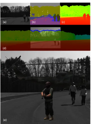
Figure 1: An example of our augmented reality driving system for military vehicle training: (a) input video frame, (b) semantic segmen-tation (different classes are represented with different colors), (c) our predicted depth map, including estimated depth information of real pedestrians (d) overlay of geo-registered video frame with a success-ful refined skyline over the 2.5D rendered image, and (e) augmented reality rendering result, including a virtual helicopter behind two real pedestrians and a virtual character. For (c)(d), depth color ranges from red to green, for small to large distance respectively.
also acquired using a LIDAR sensor and annotated in world coordi-nate beforehand. Sparse 3D global point clouds obtained from the scanning sensor can then be projected to the image perceived from a camera for enabling limited augmentations.
In this paper, we propose a new approach (Figure 1) for enabling augmented reality driving applications. Our approach significantly reduces the sensor cost required for our augmented reality driving system on each ground vehicle1by using a monocular camera in-stead of expensive 3D scanning sensors. Each 2D video frame
cap-1The current solution (LIDAR, GPS, and other sensors) in automotive industry on each ground vehicle typically costs more than $10,000: For ex-ample, Velodyne’s LIDAR on Google’s self-driving car costs at least $8,000. The total sensor cost for our solution (a monocular camera, non-differential GPS, and a low-cost IMU) on each ground vehicle is less than $2,000.
IEEE Virtual Reality 2018
18-22 March 2018, Reutlingen, Germany © IEEE 2018
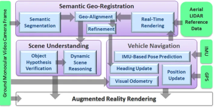
Figure 2: The architecture and data flow for all modules in our aug-mented reality system. Note the refinement procedure in semantic geo-registration module is not always successful to provide heading measurements. However, our vehicle navigation module is able to propagate opportunistic heading corrections through IMU dynamics over time to improve overall accuracy.
tured from the ground vehicle is geo-registered within the 2.5D ren-dered image from 3D geo-referenced data2, by utilizing its semantic information extracted using a pre-trained deep learning network.
For each video frame, our semantic geo-registration process (Figure 2) aligns a semantic segmentation of the video frame (each pixel is labeled as one of 12 different semantic classes) and the ren-dered depth map from 3D geo-referenced data based on our pre-dicted vehicle pose. Our scene understanding module then per-forms 3D reasoning and generates a full depth map for the input video frame. The rendered depth map provides prior information for the perceived 3D environment, but it may be outdated and does not reveal dynamic objects and temporal entities. This module clas-sifies the segmented regions using 3D reasoning techniques and computes the depth for regions representing objects that do not ex-ist in the rendered reference depth map. The rendered depth map is also updated to reflect 3D scene changes over time. In this way, more accurate and dense depth maps are generated to represent the real 3D environment perceived from the camera. As shown from our experimental results, depth for objects up to 120 meters can be estimated for driving applications.
The semantic geo-registration process in our system (Figure 2) also provides opportunistic3 global heading measurements to our vehicle navigation module, using a skyline refinement procedure. By fusing these measurements with other low-cost sensors, includ-ing non-differential GPS and an IMU (inertial measurement unit), our vehicle navigation module is able to propagate these global heading corrections though motion dynamics over long time pe-riods to improve estimates of 6 DOF (degrees of freedom) global poses of the vehicle. It is also able to generate a reliable IMU-based pose prediction for each incoming video frame quickly enough for low-latency augmented reality systems.
The remainder of this paper begins with a discussion of re-lated work in Section 2. Section 3 introduces our semantic geo-registration module, which aligns each 2D video frame perceived during driving with 3D reference data. Section 4 describes our ve-hicle navigation module, including how to fuse opportunistic global heading measurements. Section 5 shows how our scene understand-ing module generates the depth map for dynamic objects in 3D real scene. Section 6 explains how our augmented reality rendering module combines depth maps and input video frames for realistic augmentations through in-car display devices.
2Our 3D reference data was acquired using an airbone LIDAR sensor and annotated in world coordinate beforehand.
3The global heading measurement is only generated when sufficient por-tions of the skyline are observed.
In Section 7, we evaluate our system against a state-of-the-art outdoor augmented reality system, which has been used for military vehicle training [5] and observer training [18, 19]. We show our approach improves both navigation accuracy and depth map qual-ity for driving within vehicle training environments and urban ar-eas (including dense and crowded places, such as downtown streets with buildings and traffic). We also discuss the limitation of our system. Conclusions are made in Section 8.
2 RELATEDWORK
In this section, we provide a brief overview of related work to our system (Figure 2) to produce a realistic augmented reality view.
2.1 Navigation for Augmented Reality Driving
The demanding navigation accuracy requirements for augmented driving reality systems can be meet by fusing high precision dif-ferential GPS with high-end IMU sensors, or using LIDAR sensor data to geo-localize the vehicle within a pre-built geo-referenced map. However, both solutions are prohibitively expensive for com-mercial applications.
There are recent methods that fuse feature tracks [5, 10, 18, 19] perceived from low-cost monocular cameras with low-cost IMUs to filter corrupted GPS readings and to improve motion estimation over time for outdoor augmented reality applications. The closest work to our system is [5], which leverages the navigation algorithm from [18, 19] to provide precise and stable real-time 6-DOF pose estimation for military vehicle training.
However, unlike our system, all these works cannot obtain abso-lute measurements other than GPS to improve global pose estima-tion. They also do not consider either 3D reconstruction or semantic interpretation to apply dynamic occlusion of objects for an accurate augmented environment.
2.2 Image-Based Geo-Registration
The literature on image-based geo-localization is large. One gen-eral approach that closely relates to our work registers the input 2D image to untextured 2.5D geo-referenced maps, such as digi-tal elevation models from 2D cadastral maps with building height information. Among of all the sources for untextured 2.5D geo-referenced maps, LIDAR provides direct 3D sensing and relatively dense sampling of the environment. There are many methods [2, 14] that match features such as building outlines and skylines between the input image and geo-referenced model from LIDAR data. These methods either match all possible locations or search over a feature database that covers the entire target area. In con-trast, we utilize a predicted pose from our navigation module for direct alignment and then refine the pose by matching skyline ob-servations.
Related to our approach, there are also works which use an ini-tial pose followed by pose refinement. For example, Arth et al. [1] aligns straight line segments and 2.5D city map model to refine the pose. Karlekar et al. [12] refines a pose by matching a ren-dered 3D model to an input 2D image. However, these methods are only used for initialization [1, 12] in pedestrian SLAM (simulta-neous localization and mapping) systems, allowing for slower than real-time computation, while we aim to perform geo-registration continuously in real time to fulfill the demanding requirements for augmented reality driving.
2.3 Depth Estimation of Dynamic Objects
Detecting objects in the scene and performing occlusion with 3D graphics is required for many augmented reality applications. How-ever, previous approaches all have their limits. For example, depth sensors such as stereo cameras have a very short sensing range (up to 20 meters) and cannot detect distant objects. Time of flight sen-sors also have a short sensing range, and most do not work outdoors.
Expensive 3D scanning sensors, such as LIDAR, can work outdoors (up to 120 meters) but obtain relatively sparse 3D information.
For approaches involving a monocular camera, there are SLAM methods [15, 16] that perform real-time scene reconstruction dur-ing navigation. They estimate the depth map of the current im-age through small-baseline stereo matching over temporally nearby video frames. However, they generate relatively sparse depth maps and cannot recover the absolute scale of the reconstructed scene.
In this paper, we propose a new approach using a monocular camera. We infer dynamic occlusion of objects based on semantic segmentation of the video frame using a deep learning network, and recover the depth of objects with absolute scale by comparing them to 2.5D rendered scene images generated from 3D reference data. Due to recent advances with deep learning, semantic segmentation on video frames [3, 22] can be solved with high accuracy. Our work also improves the state of the art by increasing the computational speed of semantic segmentation, so that a full high-resolution depth map can be generated for each frame from 10Hz videos in real time. Our approach is able to estimate depth for objects up to 120 meters, which is the same sensing range as expensive 3D scanning sensors.
3 SEMANTICGEO-REGISTRATION
In this section, we describe our semantic geo-registration process, which registers each 2D image to the world using a 2.5D rendered image generated from 3D geo-referenced data. As shown in Figure 2, this module contributes to both our scene understanding module and vehicle navigation module for augmented reality driving.
3.1 Real-Time Rendering
For geo-referenced data, we use 3D data acquired from an airborne LIDAR sensor instead of traditional collections from the ground. Collecting data from the ground can be cumbersome, since the ve-hicle may need to be driven around the city and must deal with traf-fic. Aerial collection can cover a large area more quickly, and ob-tained data with higher resolutions. However, due to drastic view-point changes and different modalities, matching directly between 2D ground images and 3D aerial data becomes a difficult problem. To circumvent this problem, we employ a real-time rendering system that produces 2.5D rendered images based on the predicted ground viewpoint from our vehicle navigation module. The render-ing system is able to utilize pre-collected aerial LIDAR data to gen-erate geo-referenced rendered images with proper depth and edge discontinuities, based on the given viewpoint. The viewpoint is given as a 3D global pose with possible heading range (uncertainty) predicted from our vehicle navigation module. As shown in Figure 1, the 2.5D rendered image is composed to cover a viewpoint range predicted from our vehicle navigation module.
Without having to model the structures scanned by the aerial LI-DAR (which can be a quite difficult task), our system is able to render (using a graphics API such as OpenGL) the LIDAR point cloud from any arbitrary view, simulating the pose and parameters of the real camera. This is accomplished by rendering each point in the potentially sparse LIDAR collect as a sphere whose radius is a function of distance from the virtual camera and local point den-sity. This technique produces a depth image with minimized holes, where the gaps are filled in by the adaptive radii of the spheres used to represent each point.
The rendering process is made computationally efficient by the use of GPU parallel processing. The actual generation of the point spheres takes place on the GPU during the graphics API’s fragment processing step. The generation of the spheres is accomplished on the fly and in a highly parallel manner.
3.2 Semantic Segmentation
Our system is designed to work with any pre-trained network that can generate a dense segmentation labels on video frames. We have
integrated both SegNet [3] and ICNet [22], and eventually chose SegNet because of its superior accuracy from our experiments. The SegNet architecture is an encoder-decoder network, which consists of 4 layers for both the encoder and the decoder. It labels each pixel for the input video frame into 12 different semantic class labels: Sky, Building, Pole, Road Marking, Road, Pavement, Tree, Sign Symbol, Fence, Vehicle, Pedestrian, and Bike.
Note the original computation speed of the SegNet model is slow. To fulfill our computation requirements to conduct semantic seg-mentation for each input video frame in real time, we extend the method from [21] for convolution networks to convert the SegNet model into a low rank approximation of itself, by also removing redundant kernels in each de-convolution layer.
This conversion improves the efficiency of the SegNet model: The segmentation time is improved from 160 ms to 89 ms to pro-cess one image on a Nvidia K40 GPU. Similar accuracy to the orig-inal pre-trained SegNet is maintained by fine-tuning this low-rank approximation.
3.3 Geo-Alignment
Our geo-alignment process then directly overlays the semantic seg-mentation result of the input video frame to the actual predicted region (based on predicted heading from vehicle navigation mod-ule, without uncertainty range) over the rendered depth map. Both semantic segmentation result and correspondent region on the ren-dered depth map are then sent to our scene understanding module.
3.4 Refinement
Our refinement process then further refines the registered position of semantic segmentation from Section 3.3 within the 2.5D ren-dered image from Section 3.1. Because the flight altitude during 3D aerial LIDAR data collections is typically high, there are relatively smaller number of points being sampled from vertical surfaces due to occlusions. Top surfaces of solid objects, such as roof of build-ings, are sampled with denser points in LIDAR data. To exploit these dense sampled points, we choose to derive and to use skyline features from the video images for refinement. We also installed our camera on top of the ground vehicle, from which it is easier to observe skylines in the scene.
The skyline feature can be easily extracted from the semantic segmentation of the input image, by separating the sky class and non-sky classes. It can also be directly derived from the 2.5D ren-dered image by checking the depth information. We then apply distance transform [9] on the extracted binary skyline from 2.5D rendered image to generate a distance map D, whose pixel values equal to the closet distance to the nearest skyline pixel.
The skyline extracted from the input video frame is then treated as a template T. We utilize the old, but elegant chamfer matching method [4], which naturally handles possible skyline variations due to scene changes from past reference data, to find the best alignment of T over D. The chamfer matching method is slightly modified for our process as the following formulation:
arg min k N
∑
n=1 T(in, jn)D(in+ k, jn), (1) For each possible position on D (shifted horizontally by param-eter k in pixels), it sums up the distance transform values for all N skyline pixels on T. The position with the minimum summation of distance transform values represents best alignment.Note the height of our camera to the ground is known and fixed. The estimation of roll and pitch for the camera pose, from our nav-igation module, is also reliable due to the gravity direction mea-sured by the IMU sensor. Therefore, our chamfer matching process checks only 1D correlations (along horizontal axis) over D and the horizontal shift k is also bounded by the heading uncertainty from
our pose prior (typically less than 10 degrees). Therefore, the entire process becomes extremely fast. For the best alignment position of T over D, we define a confidence value based on the overlapped percentage of skylines between T and D. If the confidence value is below a threshold (currently 75%), we treat it as a wrong match.
If the best registered horizontal position is a successful match, it is used to define a global heading measurement for the vehicle (as-suming the heading of the vehicle is the same as the camera view) for our vehicle navigation module.
4 VEHICLENAVIGATION
Our vehicle navigation module incorporates sensing information from IMU, GPS, and a monocular camera. It updates pose esti-mation at our camera frame rate (10Hz) and can provide predicted poses (IMU rate, 100Hz) for our system.
4.1 IMU Motion Model
We define the navigation state of the ground vehicle at time i as xi= {pi, vi, bi}. Each state x covers three kinds of nodes: the pose node p includes 3D translation t and 3D rotation R, the velocity node v represents 3D velocity in the world coordinate system, and bdenotes sensor-specific bias block which are varied for different sensors. Note that the 3D rotation R represents the rotation from the world coordinate system to the local body’s coordinate system, while the 3D translation t represents the position of the local coor-dinate system’s origin in the world coorcoor-dinate system. To simplify the notation, we assume all sensors have the same center, which is the origin of the body coordinate system.
A navigation state is created when a camera image comes, and we use the multi-state sliding-window filter architecture to process current and past navigation states inside a buffer. Currently we set the buffer length as 4 seconds, and marginalize old states when they move out of the buffer.
In our system, the IMU sensor produces measurements at a much higher rate (100Hz) than other sensors. We integrate these high-frequency IMU measurements, and formulate them as the underly-ing motion model across two sequential navigation states. Denotunderly-ing with ai−1:iand ωi−1:iall the accelerometer and gyroscope measure-ments collected between two consecutive navigation states (at time i− 1 and i), the way to formulate the IMU motion constraint is via integration of ai−1:iand ωi−1:i:
xi= xi−1+ ml(ai−1:i, ωi−1:i) (2) where mldenotes the function integrating the accelerations and ro-tation rates. We use the pre-integration theory [13] to perform IMU integration in the local frame at time i − 1 rather than in the global frame as used in traditional IMU mechanization [5, 18, 19]. The subscript “l” in ml denotes the fact that the integration computes quantities in the local frame. In this way, the integration computes “changes” between the state at time i − 1 and i, which are indepen-dent of the state at time i − 1.
When there are delayed measurements (such as visual measure-ments generated after refinement process in the geo-registration module) older than time i − 1 received in the buffer, our filter di-rectly propagates and updates the influence from delayed measure-ments through IMU motion inside our buffer to the estimated state at newest time (> i − 1), without the need of repeating the IMU integration at every change of xi−1.
This IMU motion model generates 6 DOF relative pose and cor-responding velocity change between time i − 1 and i. The model also tracks the IMU-specific bias as part of the state variables, as-suming a random-walk model for the IMU bias evolution. This pro-cess replaces the system dynamics with the motion derived from IMU propagation, allowing for better handling of the uncertainty propagation through the whole system.
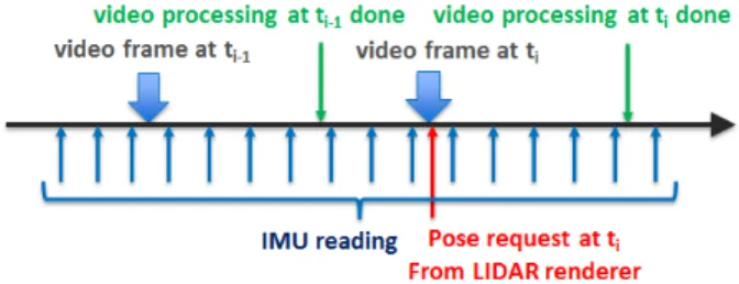
Figure 3: Timeline of pose request, prediction, and update for navi-gation state xi.
4.2 IMU-Based Pose Prediction
Our IMU motion model is also able to generate a reliable pose prediction for each incoming video frame quickly enough for low-latency augmented reality systems. As shown in Figure 3, video processing for the frame arriving at time i has not finished when the navigation state xiis created with the arrival of the video frame. The IMU motion model integrates all IMU readings between time i− 1 and i, and predicts a 6DOF pose (3D position and 3D orienta-tion) at time i by propagating relative pose change from xi−1. This approach provides the predicted pose at time i needed by the LI-DAR renderer, and the linearization point [13] for navigation state xiwhich is necessary to linearize and fuse GPS and visual measure-ments. Once the video processing for frame at time i is done, our filter is able to fuse its visual measurements and to update naviga-tion state xiin our model, improving future predictions.
4.3 Visual Odometry and GPS
Our navigation module updates the estimation of navigation states using measurements from GPS and derived from the monocular camera images. The GPS reading reports the 3D position of the moving vehicle in the world coordinate system. It directly updates the translation part t of the pose node for our navigation state.
For camera images, our system uses Harris corner detector [11] and BRIEF descriptor [6], to detect and to match visual point fea-tures across consecutive sequential frames. We also reject feature outliers using pairwise epipolar constraints and RANSAC verifica-tion [17] across frames. Our current processing time is 15 millisec-onds to process around 850 features for an image size of 640 pixels by 480 pixels using a single core of an Intel i7 CPU running at 2.80 GHz. Accepted tracked features then become measurements to update relative motion between navigation states xi−1and xi.
We also check consistency among GPS and camera measure-ments for outlier rejection. Sequential measuremeasure-ments from the same sensor needs to be consistent to the relative motion change pre-dicted from IMU model. We use this rule to verify both relative position change from sequential GPS readings and relative motion estimated from camera feature tracks across frames.
4.4 Global Heading Update
The horizontal position of successful refined skyline alignment from Section 3.4 determines a global heading angle, or equiva-lently the yaw angle for the input video frame at time i. We model this global heading reading as a measurement which updates the vehicle rotation Ri in our navigation state. In particular, we first convert the rotation matrix Rito the corresponding roll, pitch, yaw representation according to the following model, which represents this measurement z using the function h for navigation state xiwith measurement noise w:
z= h(xi) + w = yaw(Ri) + w, (3)
where yaw denotes a function that takes a 3D rotation as input and returns the corresponding yaw angle. During the update process
in our multi-state filter, in order to introduce the linearized model for (3), we note that, given a linearization point ˆRifor the current rotation, we can write (3) equivalently as:
z= h(xi) + w = yaw( ˆRiexp(θi)) + w, (4) where exp is the exponential map [7] for the rotation group which converts a 3D vector in the tangent space at the identity into a ro-tation matrix, and θi∈ R3is a rotation vector describing a rotation (also referred to as exponential coordinates). Note that the intro-duction of the exponential coordinates θiis necessary to describe small angular perturbations with respect to the linearization point
ˆ
Ri. We can now write the linearized model δ z = Jδ θi+ w, J=
∂ yaw ∂ θi
(5) Using the above model, our multi-state sliding-window filter is able to use these global heading readings to directly correct vehicle heading at video frame rate.
Note our filer is also able to propagate the influence from each global heading measurement over a long period of time in the future through IMU motion (Section 4.1). In this way, even with infre-quent global heading measurements, our vehicle navigation module is able to improve the overall navigation accuracy.
5 SCENEUNDERSTANDING
Our scene understanding module aims to recover the depth of new objects and dynamic scene with absolute scale by comparing each 2D input video frame and correspondent 2.5D rendered image (Sec-tion 3.3) from previous 3D aerial LIDAR data. It generates a full depth map for augmented realty applications, by verifying each ob-ject hypothesis from semantic segmentation (Section 3.2) and re-specting dynamic scene change from past data.
5.1 Object Hypothesis Verification
Note the semantic segmentation process (Section 3.2) labels image pixels into 12 classes. We then define these 12 classes into 5 dif-ferent categories: sky, tree, ground (road marking, road, and pave-ment), dynamic objects (vehicle, pedestrian, and bike), and static objects (building, fence, sign symbol, and pole).
We generate object candidates based on grouping segmented re-gions for dynamic objects and static objects. For each object can-didate o, we assign a true-positive flag t to the cancan-didate region m for o. t = true if the candidate region actually belongs to the object class. We then model the interaction between the object and the 3D ground plane G as p(t|m, G), which is the probability that the can-didate is true positive given the cancan-didate region m and the ground plane G. We assume the 3D ground plane is locally flat around the vehicle, and corresponds to ground semantic category in the image. The 3D ground plane can then be easily estimated based on the ground regions in the rendered depth map from 3D aerial LIDAR data. We denote the 3D ground plane as G = {n, h, f }, where n is the ground plane’s normal, h is the distance between camera and ground, and f is focal length for the camera. We then formulate
p(t = true|m, G) p(t = true|d) = N(d;0,σd), (6) This formulation shows that we use d, which is the distance be-tween object centroid to ground, to determine whether the candi-date is true instead of using G directly. We model p(t = true|d) as a Gaussian distribution with mean value 0 and sigma σd, which we learned from training data for the object class.
To estimate d, assuming we have some prior knowledge about the real scale c of the object class (such as the normal human height for pedestrian), we can approximate the distance r between object to the camera from the object height I in the image and focal length fas follows.
r'c∗ f
I , (7)
The 3D coordinate O for the centroid of object candidate o can then be approximated based on its 2d coordinate u and v as follows.
O'q r (uf)2+ (v f)2+ 1 u f v f 1 , (8)
The distance d between object centroid and the ground plane can then be computed based on the 3D coordinate O for object centroid, the ground plane’s normal n, and the distance between camera and ground h.
d= OTn+ h, (9)
Based on the above equations, the true-positive probability p(t|m, G) for each object candidate can be computed. Candidates with probability bigger than our defined threshold pass our verifi-cation. We then estimate the depth for each object, by propagating absolute depth values from the rendered ground plane to the object through the intersection between them. Simple 3D class models with techniques from [8] are used for depth propagation.
As shown in Figure 1, our hypothesis verification process is able to filter out incorrect object candidates from semantic segmentation, such as the yellow poles in Figure 1(b). Only two pedestrians pass the verification and their depth values are generated. False positive candidates all get rejected.
5.2 Dynamic Scene Reasoning
The current perceived scene may change across time for the same environment. The reference data may be outdated and does not reveal new information. For example, trees may grow and there may be new poles which do not exist before, as shown in Figure 4. Pedestrians can also appear or move out of the scene.
Therefore, in addition to depth estimation for object categories in Section 5.1, we also update the rendered depth map to reflect scene changes for other three categories: sky, tree, and ground. Since the segmentation accuracy [3] for these three categories (especially sky) is very high, we simply accept all segmented labels for these three categories to update the depth map. The depth value for sky pixels is assigned to infinity, while the depth values for pixels of ground categories can be estimated by the 3D ground plane in Sec-tion 5.1. For any pixel with the tree label, if the rendered depth value is infinity (originally sky), we assign its depth value by sam-pling nearby trees.
After our module estimates depth for new objects and changed scene, a final full high-resolution depth map for the input video frame can be used to fuse rendered elements with the real world for augmented reality applications.
6 AUGMENTED REALITY RENDERING THROUGH DISPLAY
DEVICES
Our augmented reality rendering module (Figure 2) combines both the full depth map from our scene understanding module and the predicted pose from our vehicle navigation module from each in-coming video frame for realistic augmentation. It is built using the Unity 3D game engine, which allows for easy inclusion of animated characters and effects that add to the realism of the generated scene. For each incoming video frame, this module first copies the orig-inal video imagery from the camera and requests the predicted cam-era pose from vehicle navigation module. It also loads the full depth map predicted from our scene understanding module into the depth buffer. To ensure pixels on virtual items blocked by real objects will be occluded, virtual entities or effects are then rendered to the scene using the depth buffer and received camera pose.
Figure 4: One example for object hypothesis verification and dynamic scene reasoning. Top row (left to right) shows input image, original rendered depth map, and the overlay. Bottom row shows its semantic segmentation, final depth map, and the final overlay. Depth color ranges from red to green, for small to large distance respectively. There are new poles and tree height changes from past reference in the final depth map and final overlay.
Figure 5: Selected global heading measurements from successful skyline refinements based on two different thresholds of matched skyline percentage in a Training Field sequence (x-axis: video frame index, y-axis: heading angle in degree): Blue - ground truth heading along the video sequence, Green: estimated heading from success-ful skyline refinements based on 90% matched percentage, Red: es-timated heading from successful skyline refinements based on 75% matched percentage. Note green points are a subset of red points.
We currently use a monitor inside the vehicle as the display de-vice to show augmented live videos during driving. For military training [5], this monitor is integrated as the FCD (Fire Control Unit) display for the gunner inside a Stryker vehicle. The aug-mented entities and effects in the real scene allow the gunner to learn weapon operations anywhere and anytime in live tactical sit-uations, and do not require significant facilities and range infras-tructure at specific sites with safety restrictions. For automotive in-dustry, augmented live videos can be shown through in-car head-up displays (HUD) [20] for applications such as driver assistance.
7 EXPERIMENTS
Our augmented reality driving system incorporates a low-cost non-differential GPS, a 100Hz MEMS Microstrain GX4 IMU, and one 10Hz front-facing monocular Point Grey camera on the vehicle for experiments. To evaluate the accuracy from our augmented reality system, we also installed an expensive high-precision differential GPS, which was used only for generating 6 DOF global pose (fused with IMU) for the vehicle as ground truth. All sensors are calibrated and triggered through hardware synchronization. The computation hardware for our system is a Gygabyte Brix gaming/ultra-compact computer with Intel i5 CPU and NVIDIA GPU.
We validate our approach against our own implementation of a state-of-the-art outdoor augmented reality system [5, 18, 19], which has been used for military vehicle training and observer training. Although this system incorporates the same set of sensors as our system, its filter architecture and IMU mechanism formulation are different from our system (Section 4.1). It does not perform geo-registration to improve pose estimation, and does not consider 3D
Figure 6: Skyline refinement examples (two successful cases, and two failed cases with less than 75% skyline are perceived) on down-town streets during one urban city driving sequence (blue trajectory on google earth: 5.08 kilometers, 12 minutes).
scene reconstruction for producing more realistic augmentations. We conduct experiments on two environments to evaluate perfor-mance from four perspectives: heading refinement precision, navi-gation accuracy, depth map quality, augmented rendering quality.
The first environment is a training field, including unpaved roads and country roads, which is similar to [5, 18, 19] for military train-ing. There are 4 sequences: each sequence is around 5.5 minutes and 3.1 kilometers. The driving speed can be as high as 60 mph (miles per hour), but it is usually between 20~50 mph.
The second environment is a large-scale urban city. It includes dense and crowded places, such as downtown streets with a variety of buildings and traffic, which are more challenging. There are 3 se-quences: each sequence is around 12 minutes and 5.08 kilometers. The driving speed is mostly slow (10~20 mph) due to the traffic.
7.1 Heading Refinement Precision
We first evaluate our skyline refinement process (Section 3.4) in geo-registration module. Note we compute the matched skyline percentage for each skyline refinement, and use it as the threshold for selection. Currently we choose 75% as the threshold, which gets much more successful matches during driving (comparing to 90%, as shown in Figure 5). More than half of video frames get success-ful skyline refinements in training field, and the median error of the selected heading measurements is 1.2944 degree.
However, as shown in Figure 6, the skyline refinement procedure (Section 7.1) fails more often in urban city, because the skyline in the camera scene is easier to be occluded due to a variety of buildings or trees. The percentage of video frames with successful skyline refinements decreases to 36.97% over 5 km driving. The median error of selected heading measurements is 0.9850 degree.
7.2 Navigation Accuracy
We compare our performance against a baseline system and the sys-tem from [5, 18, 19] to evaluate the navigation accuracy of our augmented reality system during driving. The baseline system is a simplified version of our system: It generates results from our vehicle navigation module without using global heading measure-ments (Section 4.4). Both our baseline system and the system from [5, 18, 19] fuse only feature track measurements from the monocu-lar camera and do not perform geo-registration.
As shown in Figure 7, global heading measurements improves the heading estimation for navigation accuracy in our system over our baseline system and the system from [5, 18, 19]. Using our rendering system with display devices, we found estimated heading error less than 2 degrees is required for producing realistic augmen-tations. Other two systems are unable to generate global heading estimation with such required accuracy in urban city, especially on downtown streets (the heading error is more than 4 degrees).
By fusing global heading measurements with other sensor mea-surements (non-differential GPS, IMU, and feature tracks), the final
Figure 7: Statistical analysis of heading error (y-axis in degrees) among 3 systems (x-axis: 1- our system, 2- our baseline system, 3- the system from [5, 18, 19]) over two environments (left: training field, right: urban city).
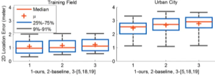
Figure 8: Statistical analysis of 2d location error (y-axis in meters) among 3 systems (x-axis: 1- our system, 2- our baseline system, 3-the system from [5, 18, 19]) over two environments (left: training field, right: urban city).
heading estimation from our system is even more accurate than the global heading measurement itself. For example, on training field, the median heading error (0.439 degree) from our final pose es-timation is smaller than the median error (1.2944 degree) for our heading measurements from successful skyline refinements. How-ever, although our navigation module leverages infrequent skyline refinement measurements in urban city to improve overall heading accuracy, heading error still increases to 2 degrees if we drive at crowded places for a long period of time.
The global heading measurements also further influence posi-tion variables through moposi-tion propagaposi-tion within our filter (Figure 8). We also use terrain height from geo-referenced data to correct the height in our estimated pose. Therefore, the error from our esti-mated position is mainly from the horizontal direction.
7.3 Depth Map Quality
Our scene understanding module is able to construct a reasonable full depth map, including dynamic objects and changed scenes, for each input video frame. Note our module generates a dense high-resolution depth map for each input 2D video frame, with depth estimation of dynamic objects up to 120 meters (based on the min-imum size of detected far-away objects on the 3D ground plane). This allows the user to have sufficient time to perceive the aug-mented information for response during high-speed driving. Figure 9 shows examples on the training field. We also annotate the esti-mated depths for pedestrians and cars, which are beyond the sensing range limitation (up to 20 meters) from stereo cameras and time-of-flight sensor. Our system is able to estimate the depths for these far-away objects, which is required to handle dynamic occlusion for enabling realistic augmentation.
Figure 10 shows examples on downtown streets in the urban city. The perceived scene includes other vehicles and a variety of build-ings on the side. Depth of all cars in the scene is estimated in final depth maps. However, the quality of our estimated depth maps also decreases in dense areas, due to the reduced accuracy of SegNet [3]
Figure 9: Examples on the depth map including far-away dynamic objects using our system on the training field: (left to right) input image, semantic segmentation, and final depth map with scene un-derstanding. Depth color ranges from red to green, for small to large distance respectively. We also annotate the estimated depth for far-away pedestrians or vehicles on the pictures in depth maps. Note our system still detects two far-away pedestrians and estimates their depth in the last example. We mark the regions for these two people (also enlarge it on the input image) for visualization.
for crowded scenes.
7.4 Augmented Rendering Quality
Our system creates augmentations (Section 6) on live video feeds, by utilizing the global pose (position and orientation) from our ve-hicle navigation module and the depth map from our scene under-standing module. Figure 11 shows snapshots over our two evalu-ated environments (training field, urban city) from our augmented videos during driving. The inserted virtual objects are placed pre-cisely and appear stable in the driver’s view. On the training field, the occlusion relationship between virtual helicopters and real ob-jects (pedestrians and the bush) is also maintained correctly for re-alistic visualization using depths estimated from our system.
Note the system from [5, 18, 19] fails to produce realistic aug-mentations for either of these two situations in Figure 11: It cannot handle occlusion relationship on training fields, and is unable to estimate accurate global heading on downtown streets.
8 CONCLUSIONS
We propose an effective and inexpensive approach to fulfill two major requirements for augmented reality driving applications: Es-timating precise 6 DOF global pose of the vehicle, and reconstruct-ing 3D dynamic scenes perceived from the vehicle camera. Our approach directly extracts the semantic information from a monoc-ular video camera using a pre-trained deep learning network, and is registered to 2.5D images rendered from 3D geo-referenced data.
The geo-registration process provides opportunistic global head-ing measurements to our vehicle navigation module to improve its estimation of global pose over state-of-the-art augmented reality systems [5, 18, 19]. Our scene understanding module generates a full depth map for each video frame, by combing its semantic segmentation and the predicted rendered depth map from 3D refer-ence data. It computes depth for dynamic objects up to 120 meters, and updates 3D scene changes over time. The combination of ve-hicle poses and depth maps using our approach enables realistic augmented reality driving experience, especially on training fields. To extend our system beyond applications for military vehicle training, we need to improve our system specifically for dense and crowded urban environments. We plan to extract a larger variety of features from both input images and reference data to derive more frequent global measurements from our geo-registration process. We also plan to improve semantic segmentation accuracy, by train-ing more data from crowded urban environments.
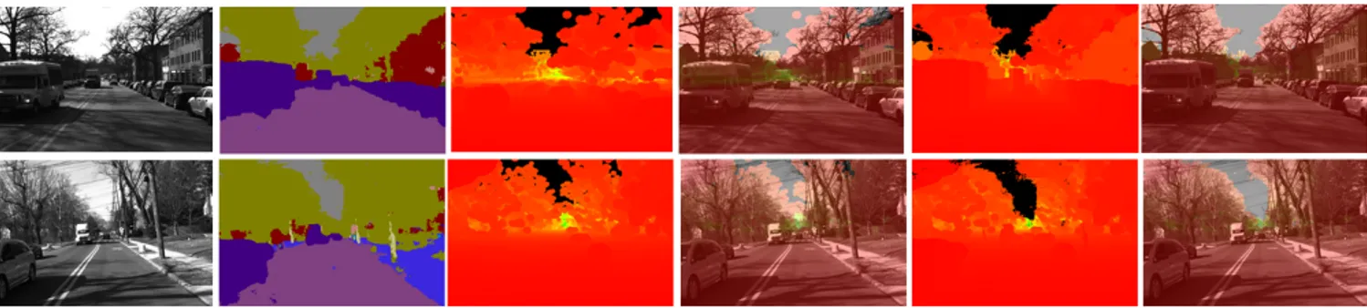
Figure 10: Examples on the depth map quality using our system on downtown streets in urban city: (left to right) input image, semantic segmen-tation, rendered depth map without scene understanding, overlay without scene understanding, final depth map with scene understanding, and overlay with scene understanding. Depth color ranges from red to green, for small to large distance respectively.
Figure 11: Snapshots over our two evaluated environments from our augmented reality videos perceived during driving. The first two snapshots (training field) show inserted virtual helicopters behind two real pedestrians and the bush respectively. The final two snapshots (urban city) show inserted virtual characters on downtown streets.
REFERENCES
[1] C. Arth, C. Pirchheim, J. Ventura, D. Schmaistieg, and V. Lep-etit. Instant outdoor localization and slam initialization from 2.5d maps. IEEE Transations on Visualization and Computer Graphics, 21(11):1309–1318, November 2015.
[2] G. Baatz, O. Saurer, K. Koser, and M. Pollefeys. Large scale vi-sual geo-localization of images in mountainous terrain. In The Eu-ropean Conference on Computer Vision (ECCV’12), pages 517–530. Springer, 2012.
[3] V. Badrinarayanan, A. Handa, and R. Cipolla. Segnet: A deep convo-lutional encoder-decoder architecture for robust semantic pixel-wise labelling. arXiv preprint arXiv:1505.07293, 2015.
[4] H. Barrow, J. Tenebaum, R. Bolles, and H. Wolf. Parametric cor-respondence and chamfer matching: Two new techniques for image matching. In International Conference of Artifical Intelligence (IJ-CAI’77), pages 659–663, 1977.
[5] J. Brookshire, T. Oskiper, V. Branzoi, S. Samarasekera, and R. Ku-mar. Military vehicle training with augmented reality. In In-terservice/Industry Training, Simulation, and Education Conference (I/ITSEC15), 2015.
[6] M. Calonder, V. Lepetit, C. Strecha, and P. Fua. BRIEF: binary robust independent elementary features. In European Conference on Com-puter Vision (ECCV’10). Springer, 2010.
[7] L. Carlone, K. Daniilidis, and F. Dellaert. Initialization techniques for 3d slam: a survey on rotation estimation and its use in pose graph optimization, 2015.
[8] H. Chiu, H. Liu, L. Kaelbling, and T. Lozano-Perez. Class-specific grasping of 3d objects from a single 2d image. In IEEE/RSJ Interna-tional Conference on Intelligent Robots and Systems (IROS’10), pages 579–585. IEEE, 2010.
[9] P. Felzenszwalb and D. Huttenlocher. Distance transforms of sampled functions. Theory of Computing, 8(19), 2012.
[10] E. Foxlin, T. Calloway, and H. Zhang. Improved registration for vehic-ular ar using auto-harmonization. In IEEE International Symposium on Mixed and Augmented Reality (ISMAR’14), pages 105–112. IEEE, 2014.
[11] C. Harris and M. Stephens. A combined corner and edge detector. In
Proc. of Fourth Alvey Vision Conference, 1988.
[12] J. Karlekar, S. Zhou, W. Lu, Z. Loh, and Y. Nakayama. Position-ing, tracking and mapping for outdoor augmentation. In IEEE Inter-national Conference on Mixed and Augmented Reality (ISMAR’10), pages 175–184. IEEE, 2010.
[13] T. Lupton and S. Sukkarieh. Visual-inertial-aided naivgation for high-dynamic motion in built environments without initial conditions. IEEE Transactions on Robotics, 28:61–76, 2012.
[14] B. Matei, N. Valk, Z. Zhu, H. Cheng, and H. Sawhney. Image to lidar matching for geotagging in urban environments. In IEEE Winter Conference on Applications of Computer Vision (WACV’13), pages 413–420. IEEE, 2013.
[15] R. Mur-Artal, J. Montiel, and J. Tards. Orb-slam: A versatile and accurate monocular slam systems. IEEE Trans. Robotics, 31(5):1147– 1163, 2015.
[16] R. Mur-Artal, J. Montiel, and J. Tards. Orb-slam2: An open-source slam system for monocular, stereo, and rgb-d cameras. IEEE Trans. Robotics, 33(5):1255–1262, 2017.
[17] D. Nister. Preemptive ransac for live structure and motion estimation. In IEEE Intl. Conf. on Computer Vision (ICCV’03). IEEE, 2003. [18] T. Oskiper, S. Samarasekera, and R. Kumar. Multi-sensor
naviga-tion algorithm using monocular camera, imu, and gps for large scale augmented reality. In IEEE International Symposium on Mixed and Augmented Reality (ISMAR’12), pages 71–80. IEEE, 2012. [19] T. Oskiper, S. Samarasekera, and R. Kumar. Augmented reality
binoc-ulars on the move. In IEEE International Symposium on Mixed and Augmented Reality (ISMAR’14), pages 289–290. IEEE, 2014. [20] B. Park, J. Lee, C. Yoon, and K. Kim. Augmented reality for collision
warning and path guide in a vehicle. In The ACM Symposium on Vir-tual Reality Software and Technology (VRST’15), page 195, Beijing, China, 2015. ACM.
[21] C. Tai, T. Xiao, Y. Zhang, X. Wang, and E. Weinan. Convolutional neural networks with low-rank regularization. In International Con-ference on Learning Representations (ICLR’16), 2016.
[22] H. Zhao, X. Qi, X. Shen, J. Shi, and J. Jia. Icnet for real-time semantic segmentation on high-resolution images. arXiv preprint arXiv:1704.08545, 2017.