ADE-4
Multiple correspondence
analysis
Abstract
This is an introduction to the analysis of tables containing categorical (qualitative) data. In this case, values are represented by modalities. These modalities can be ordered resulting in an ordinal coding. In this volume we perform a multiple correspondence analysis on a data set dealing with cat's fecundity (Pontier, 1984, Contribution à la biologie et à la génétique des populations de chats domestiques (Felis catus). Thèse de 3° cycle. Université Lyon 1. 1-145).
Contents
1 - Data set... 2
2 - Description of qualitative variables... 3
3 - Computation... 5
4 - Interpretation... 9
Références ... 12
1 - Data set
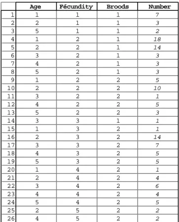
The data used to illustrate this analysis are those recorded by D. Pontier 1. Table 1 contains three columns corresponding to three qualitative variables and 26 rows. Each row represents a group of cat females having the same modalities for the three variables. The fourth column indicates the number of cat females in each group.
Table 1 Data analysed in this volume.
Age Fécundity Broods Number
1 1 1 1 7 2 2 1 1 3 3 5 1 1 2 4 1 2 1 18 5 2 2 1 14 6 3 2 1 3 7 4 2 1 3 8 5 2 1 3 9 1 2 2 5 10 2 2 2 10 11 3 2 2 1 12 4 2 2 5 13 5 2 2 3 14 3 3 1 1 15 1 3 2 1 16 2 3 2 14 17 3 3 2 7 18 4 3 2 5 19 5 3 2 5 20 1 4 2 1 21 2 4 2 4 22 3 4 2 6 23 4 4 2 4 24 5 4 2 5 25 2 5 2 2 26 4 5 2 2
The first column indicates the age of cats. Modalities correspond to
1: 1 year old she cats 4: 6 or 7 years old she cats 2: 2 or 3 years old she cats 5: 8 years old she cats 3: 4 or 3 years old she cats
The second column indicates the number of kittens born over one year. This is a consequently a measurement of fecundity:
1: 1 or 2 kittens 4: 9 to 12 kittens 2: 3 or 6 kittens 5: 13 or 14 kittens 3: 7 or 8 kittens
The number of broods per year, recorded in the third column, is identified as follows:
1: one brood 2: two broods
The aim of the analysis is to separate the modalities of variables in the best way and to recognise groups of cat females according to their fecundity features. Multiple correspondence analysis (see a review in Tenenhaus & Young, 1985)2 aims to generate quantitative scores, which maximise the mean correlation ratio among qualitative variables. Consequently this method is well designed for categorical data sets.
Create a data folder and go to the ADE•Data selection card. Select « ChatBis » in the right-hand data menu. The following ADE•Data card shows up:
Copying the data results in the two following files: Chat.txt and ChatEff.txt. For
English natives, this files may be replaced by Felix.txt and FelixNum.txt.
Use the appropriate option of the TextToBin module to transform these text files into binary files (Felix (26-3) and FelixNum (26-1)):
---Option: Excel-Binary
Input text file: Chat.txt
---Row 1 Words 3 : 1◊1◊1
Row 2 Words 3 : 2◊1◊1 ...etc.
78 numbers found in file Chat.txt Row number: 26 Column number: 3
---Output binary file Felix
---Option: Excel-Binary
Input text file: ChatEff.txt
---Row 1 Words 1 : 7
Row 2 Words 1 : 3 ...etc.
26 numbers found in file ChatEff.txt Row number: 26 Column number: 1
---Output binary file FelixNum
---2 - Description of qualitative variables
To use a binary file that contains categorical variables, the number of categories for each variables and the number of sampling units for each category must be stored in an auxiliary file.
Use the CategVar module with the Read Categ File option to describe the content of the file Felix. This program generates an auxiliary file noted ----.Cat.
************************************ * Description of a coding matrix * ************************************ Categorical variables: file Felix
Rows: 26, Variables: 3, Categories: 12, Missing data: 0 Description of categories:
---Variable number 1 has 5 categories
---[ 1]Category: 1 Num: 5 Freq.: 0.192 [ 2]Category: 2 Num: 6 Freq.: 0.231 [ 3]Category: 3 Num: 5 Freq.: 0.192 [ 4]Category: 4 Num: 5 Freq.: 0.192 [ 5]Category: 5 Num: 5 Freq.: 0.192 Variable number 2 has 5 categories
---[ 6]Category: 1 Num: 3 Freq.: 0.115 [ 7]Category: 2 Num: 10 Freq.: 0.385 [ 8]Category: 3 Num: 6 Freq.: 0.231 [ 9]Category: 4 Num: 5 Freq.: 0.192 [ 10]Category: 5 Num: 2 Freq.: 0.0769 Variable number 3 has 2 categories
---[ 11]Category: 1 Num: 9 Freq.: 0.346 [ 12]Category: 2 Num: 17 Freq.: 0.654
---Auxiliary binary output file FelixModa: Indicator vector of modalities
It contains variable number for each modality It has 12 rows (modalities) and one column
Auxiliary ASCII output file Felix.123: labels (two characters) for 12 modalities
It contains one label for each modality
It has 12 rows (modalities) and labels 1a,1b, ..., 2a, 2b, ...
Variable number 1,2, ..., A, ..., Z,+, Modality number a,b, ..., z,+
---Num (number) indicates the number of rows (groups of females) having the same modality for a given variable (S Num equal 26 for one variable). Freq (frequency) represents the percentages of rows (groups of females) having the same modality (S Freq equal 1 for one variable). One should not that these percentages do not represent the percentages of individuals (cat females) having the same modality. These percentages will be used as the weight in this analysis, from now on, they will be called weight. In the case of non weighting file (one individual per row) frequency and weight are identical
File Felix.cat contains: the number of rows (26), the number of variables (3), the number of categories (12), the category number by variable, the row number by category.
File FelixModa contains values that identify to which variable a modality belongs to as follows: Row: 12 Col: 1 1 | 1.0000 | 2 | 1.0000 | 3 | 1.0000 | 4 | 1.0000 | 5 | 1.0000 | 6 | 2.0000 | 7 | 2.0000 | 8 | 2.0000 | 9 | 2.0000 | 10 | 2.0000 | 11 | 3.0000 | 12 | 3.0000 |
File FelixModa.cat is a text file that contains a description of FelixModa: 12 (total number of categories)
1 (number of variable (1) of FelixModa)
3 (total number of categories of the variable 1) 3 (number of categories of the variable 1)
5 (category number of the first variable) 5 (category number of the second variable) 2 (category number of the third variable)
Theses files are used for specific graphical representations. Files Felix.123 and FelixModa.123 represent labels files.
Files ---.cat (i.e., Felix.cat) are used for the computation and serves to indicate that file --- (i.e., Felix) contains category numbers.
The Read Categ File module is very useful to examine accurately the content of qualitative files (especially when the number of records is large). The description of the frequency of each modality may lead to their new coding for example in the case of missing modalities or when they have a very low frequency.
3 - Computation
Run the MCA module with the Multiple Correspondence Analysis option:
As usual, the inertia ratio of each axis, the cumulated inertia and the following eigenvalues diagram show up:
Select one axis because the above graph shows that the first axis well describes the data structure. Save the listing to get information about the results of this computation:
Row weights from file FelixNum
File Felix.cmpl contains the row weights It has 26 rows and 1 column
File Felix.cmpc contains the column weights (1/V)*DM It has 12 rows and 1 column
Marginal distributions by variable:
---Variable number 1 has 5 categories
---[1] Category: 1 Weight: 0.239 [2] Category: 2 Weight: 0.351 [3] Category: 3 Weight: 0.134 [4] Category: 4 Weight: 0.142 [5] Category: 5 Weight: 0.134 Variable number 2 has 5 categories
---[6] Category: 1 Weight: 0.0896 [7] Category: 2 Weight: 0.485 [8] Category: 3 Weight: 0.246 [9] Category: 4 Weight: 0.149 [10] Category: 5 Weight: 0.0299 Variable number 3 has 2 categories
---[11] Category: 1 Weight: 0.403
[12] Category: 2 Weight: 0.597
---File Felix.cmta contains the table processed by MCA It has 26 rows and 12 columns (categories)
---DiagoRC: General program for two diagonal inner product analysis Input file: Felix.cmta
--- Number of rows: 26, columns: 12
---Total inertia: 3
---Num. Eigenval. R.Iner. R.Sum |---Num. Eigenval. R.Iner. R.Sum | 01 +7.0114E-01 +0.2337 +0.2337 |02 +4.1772E-01 +0.1392 +0.3730 | 03 +3.7837E-01 +0.1261 +0.4991 |04 +3.4426E-01 +0.1148 +0.6138 | 05 +3.2456E-01 +0.1082 +0.7220 |06 +2.8872E-01 +0.0962 +0.8183 | 07 +2.5132E-01 +0.0838 +0.9020 |08 +2.0156E-01 +0.0672 +0.9692 | 09 +9.2342E-02 +0.0308 +1.0000 |10 +0.0000E+00 +0.0000 +1.0000 | 11 +0.0000E+00 +0.0000 +1.0000 |12 +0.0000E+00 +0.0000 +1.0000 | File Felix.cmvp contains the eigenvalues and relative inertia for each axis
--- It has 12 rows and 2 columns
File Felix.cmco contains the column scores --- It has 12 rows and 1 columns
...etc. File Felix.cmli contains the row scores
--- It has 26 rows and 1 columns
...etc. CorRatioMCA: Correlation ratios after a MCA
Title of the analysis: Felix.cm Number of rows: 26, columns: 3 Variable : 1 > Categ= 1 Weight= 0.239 -1.235 > Categ= 2 Weight= 0.351 0.083 > Categ= 3 Weight= 0.134 0.871 > Categ= 4 Weight= 0.142 0.695 > Categ= 5 Weight= 0.134 0.374 ---> r= 0.556 Variable : 2 > Categ= 1 Weight= 0.090 -1.540 > Categ= 2 Weight= 0.485 -0.578 > Categ= 3 Weight= 0.246 0.937 > Categ= 4 Weight= 0.149 1.056 > Categ= 5 Weight= 0.030 1.002 ---> r= 0.787 Variable : 3 > Categ= 1 Weight= 0.403 -1.062 > Categ= 2 Weight= 0.597 0.717 ---> r= 0.761
File Felix.cmrc contains the correlation ratios between the categorical variables and the factor scores
It has 3 rows and 1 columns
The fact that the row weights are not uniform (weighted by the number of cats having the same combination of modalities) leads to the computation of weights for
each modality and each variable. These weights are different from frequencies calculated previously (CategVar module).
For instance, among the groups of cats the frequency of the first modality of the first variable equals 5/26 = 0.192 (the first modality is observed 5 times in the table) and the weight equals (7+18+5+1+1)/(7+3+2+18+...+5+2+2) = 32/134 = 0.239
If the row are not weighted then the row weights are uniform (1/n) and weights and frequencies are similar. In multiple correspondence analysis, the total inertia equals the number of variables (3).
[See MCA : Correlation ratio - cmta]
The use of the Quick Basic program CategCovar helps the interpretation of qualitative data as it allows the calculation of means, variances and covariances of quantitative variables for each modality of each categorical variable.
Select CategCovar via the ADE•Old selection card:
In our example, Felix.cmli is a quantitative file computed from categorical data. It contains the row scores of the raw table Felix :
Within category variance on file Qual
input file name (quantitative variables) Felix.cmli column number 1
input file name (categorical variables) Felix Output file name Fel
---Output file Fel is a non standard file
Ellipses drawing by GraphMu : it is a 12 row and 1 variable file ADE file : it is also a 12 row and 2 column file
Therein columns 1 to 1 are means and columns 2 to 2 contains the lower-half variance-covariance matrice
Rows are categories defined by Felix Variables are defined by Felix.cmli
---<Var> means variances
< 1> 0.34459E-07 0.70114E+00 Column 1 from Felix.cmli
---Var= 1 /cat= 1 Means=-.1034E+01 Varia=0.5005E-01
Var= 1 /cat= 2 Means=0.6949E-01 Varia=0.1354E+00 Var= 1 /cat= 3 Means=0.7295E+00 Varia=0.3483E-01 Var= 1 /cat= 4 Means=0.5819E+00 Varia=0.3445E-01 Var= 1 /cat= 5 Means=0.3130E+00 Varia=0.5673E-01 Correlation ratio= 0.5558
---Var= 2 /cat= 1 Means=-.1289E+01 Varia=0.7215E-02
Var= 2 /cat= 3 Means=0.7844E+00 Varia=0.8933E-02 Var= 2 /cat= 4 Means=0.8843E+00 Varia=0.5572E-02 Var= 2 /cat= 5 Means=0.8390E+00 Varia=0.4429E-03 Correlation ratio= 0.7869
---Var= 3 /cat= 1 Means=-.8890E+00 Varia=0.6522E-01
Var= 3 /cat= 2 Means=0.6000E+00 Varia=0.1025E+00 Correlation ratio= 0.7608
---The above listing permit to verify that the row scores are centred (mean equal 0, in bold) and their total variance is equal to the first eigenvalue of the MCA (λ1=0.7011) also equal to the average correlation ratio. MCA aims to compute a score for individuals (groups of same individuals) that enable the maximisation of the average correlation ratio.
The column scores (Felic.cmco) are computed from the above mean values as follows for example for the first modality of the first variable (in bold):
−1.034× 1
0.701= −1.235
This means that using MCA, a modality is positioned at the weighted average scores of groups of individuals that represent the modality at about a coefficient equal to 1
k
.
The correlation ratio are computed for each variable (resulting either from the MCA module or from CategCovar Quick Basic program) and are useful to recognise easily which variables are taken into account by a given axis. By definition, it is the ratio of the computed quantitative scores to a qualitative variable. Thereby, for one qualitative variable, it is the ratio of the between-modality variance (i.e., variance of the means scores of individuals that present a category, see above) to the total variance (i.e., variance of individual scores whatever the category considered).
The values of correlation ratios variables-axes for the first axes (associated with the higher eigenvalues) can be used to investigate the relationships between modalities. As a result, 56% of the variance of individual scores on the first axis represent the between modality variance of the first qualitative variable, 79% represent the between modality variance of the second qualitative variable, and 76% is the between modalities variance of the third qualitative variable.
4 - Interpretation
The eigenvalues graph can be drawn with the Curves module (Bars option) as follows:
0 0.71
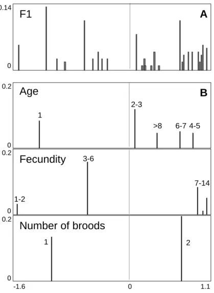
A synthetic view results from the drawing of the dispersion of individuals (groups of cat females in Fig. 1A) and the distribution of modalities according to their scores on the first axis (Fig. 1B). To get Fig. 1A, use the Curves module with the Bars option and fill the dialog boxes as follows:
To get Fig. 1B, use the same module with the same option and fill the dialog boxes as follows:
File Felix.cmpc contains the column weights that represent the weight of a modality (see above) divided by the number of variables.
Use the file FelixModa.cat to select the modalities according to the variable to which they belong (Row & col. selection in the Windows popmenu) as follows:
F1
0 -1.6 1.1Number of broods
2 1 0.2 0Fecundity
1-2 3-6 7-14 0.2 0Age
1 2-3 >8 6-7 4-5 0.2 0 0.14 0A
B
Figure 1 A - Factorial scores of individuals (groups of cat females) on the first axis are used as abscissa (individuals are situated at the weighted average of the modalities they present, at about a dilatation coefficient). Bars are proportional to the individual weights. B - The 12 modalities grouped by variable; factorial scores of modalities on the first axis are used as abscissa (modalities are at the weighted average of individuals that present these modalities at about a dilatation coefficient). Bars are proportional to the modality weights.
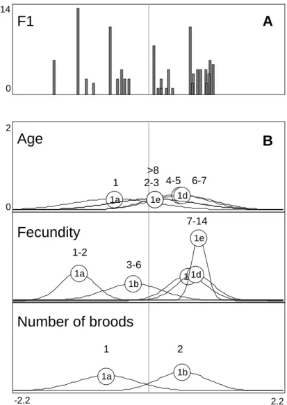
Another illustration of the results using Gauss curves (i.e., adding a dispersion to Fig. 1) may be drawn (Fig. 2). Gauss curves are built using the conditional means and variances of each modality computed from CategCovar. Use the Graph1DClass module with Gauss curves option and fill the dialog boxes as follows:
1a 1b1e 1c1d 1a 1b 1c1d 1e 1a 1b 0 2 -2.2 2.2 0 0.14
F1
Number of broods
Fecundity
Age
A
B
1-2 3-6 7-14 2 1 1 2-3 >8 6-7 4-5Figure 2 A - This graph is similar to Fig. 1A. B - Gauss curves for each modality. Modalities are grouped by variable.
Cat fecundity is different according to the age (three groups can be distinguished). Young cat female (one year old; modality 1a) have a low fecundity, i.e., one brood per year (modality 1a) with no more than two kittens (modality 1a). The reproduction begin to be actually effective when the cat female are 2-3 years old and the optimum is reached for 4-5 years old. Afterwards, the fecundity decreases; older cat females have still two broods a year, but the number of kittens is lower than earlier stages.
A similar conclusion can be reached using a different graphical viewpoint.
[See TabCat : Values]
Références
1 Pontier, D. (1984) Contribution à la biologie et à la génétique des populations de chats domestiques (Felis catus). Thèse de 3° cycle. Université Lyon 1. 1-145.
2 Tenenhaus, M. & Young, F.W. (1985) An analysis and synthesis of multiple correspondence analysis, optimal scaling, dual scaling, homogeneity analysis ans other methods for quantifying categorical multivariate data. Psychometrika : 50, 1, 91-119.