Lire la première partie
de la thèse
Chapter 7
Exploration with 2-by-2
experiments
Contents
7.1 Introduction . . . 201
7.1.1 What are 2-by-2 experiments ? . . . 201
7.1.2 Link with global sensitivity analysis . . . 203
7.2 Validation of the tuning strategy . . . 205
7.2.1 Setting σobswith wind spectrum slope . . . 205
7.2.2 Variations of the wind RMSE against the main inputs . . . 207
7.2.3 Effect of N on the execution time . . . 212
7.2.4 Tuning strategy for the reconstruction . . . 212
7.3 Other interesting results . . . 214
7.3.1 On the bad construction of the score rk . . . 214
7.3.2 Influence of C0and C1 . . . 216
7.3.3 Retrieval of known variations of NG0 . . . 221
7.4 Conclusion . . . 223
7.1 Introduction
7.1.1 What are 2-by-2 experiments ?
The idea of 2-by-2 experiments is the following. After a first work of development, a new system (denoted by a function f, such as in figure 6.1) is built and a sensitivity analysis is desired. The first phase of development usually provides a set of values for the input parameters for which the system globally works and a guess on the range in which they belong. The sensitivity analysis will explore the influence of the input parameters when they browse this range.
Sensitivity indices (such as Sobol indices) provide a quantification of the influence of an input by a single value, without any assumption on the system. But a single value is a very
short summary of the influence. The form of the function f is a much more fertile knowledge on the system because it can be interpreted.
So called "One-At-Time" (OAT) methods are very informative about the form of f. Using the nominal values and the range of variations provided by the development phase, OAT methods make one input vary while the others are set to a nominal value. By doing so, it is possible to draw the evolution of outputs when this input varies. But this method looses the effect of interactions between inputs (Saltelli and Annoni, 2010) and there is a chance that the nominal value of another input hinders the effects of the moving input.
On another hand, let all the inputs vary is the good method to catch all variations, as we have seen in sensitivity analysis. But the shape of f is not accessible when all inputs are moving. Only projections can be drawn, and they are poisoned by the variations of others parameters.
Let 2 inputs vary is a compromise to keep the drawing capacity of OAT and the possibility to take interactions into account. Such experiments are denoted as 2-by-2 experiments. It is a way to check the main features pointed out by the sensitivity analysis. The expected result is to find the mechanism at the origin of the influence in order to control it (to reduce uncertainty or to tune the system to various situations). The total experimental plan is summarized in the table 7.1, but the resulting figures are too numerous to be all included in the main matter. To make browsing easier, hyperlinks to the appendix are inside the table 7.1. The experimental plan can also be represented by a graph: vertices are input parameters and edges exists between two inputs for which a 2-by-2 experiment has been carried out. The resulting graph of the present experimental plan is shown figure 7.1. For each edge of the graph 7.1, the five outputs have been computed. The inputs connected by the edge are the only ones to move, the others stay at their nominal value. Both nominal values and ranges of variation are recap in the table 7.2.
C0 C1 ℓ N σadd σobs σV σX τ C0 p.303 p.306 C1 p.303 ℓ p.306 p.312 p.315 p.318 N p.312 p.321 p.324 p.327 σadd p.315 p.321 p.330 p.333 σobs p.318 p.324 p.330 p.336 p.339 σV p.342 σX p.336 p.342 τ p.327 p.333 p.339
Table 7.1 – Couples of inputs experimented: results are on the indicated page (hyperlink). This table is a copy of C.3.
Figure 7.1 – Graph of 2-by-2 experiments: vertices are input parameters and edges exist between inputs involved in a common 2-by-2 experiment. The annotated numbers are the degree of the vertices.
Input Min Max Nominal value Unit
C0 0.3 2.5 2.1 none C1 0 2.5 0.9 none ℓ 3 100 10 m N 400 2500 700 none σadd 0.1 2.1 0.5 m·s−1 σobs 0.1 2.1 0.5 m·s−1 σV 0 1.1 0.1 m·s−1 σX 0 11.1 1.0 m τ 5 30 10 min
Table 7.2 – Range of variation and nominal value for each input.
7.1.2 Link with global sensitivity analysis
For global sensitivity analysis, the computer code is seen as a function of all the parameters. The Hoeffding decomposition of this function allows to attribute the variance on the output to a group of parameters.
Y = f (X) =Ø u∈I
fu(Xu) (7.1)
For a 2-by-2 experiment, we look at the same function but with only two parameters moving. The others are fixed to their nominal value. The 2 parameters varying are denoted
has only 3 terms : ˜
Y = ˜f (Xi, Xj) = ˜fi(Xi) + ˜fj(Xj) + ˜fi,j(Xi, Xj) (7.2)
The two models are linked by the fixation of the parameters Xi,j ={Xk, k∈ [[1, p]], k Ó=
i, j} to their nominal value xi,j.
L( ˜Y ) =L(Y |Xi,j = xi,j) (7.3)
Because the Hoeffding decomposition is unique, one can identify the terms : ˜ fi(Xi) = Ø u∈I,i∈u fu(Xi, xu\i) (7.4) ˜ fi,j(Xi, Xj) = Ø u∈I,{i,j}∈u fu(Xi, Xj, xu\{i,j}) (7.5)
But this relationship are not exploitable without additional assumptions. The main inter-est of 2-by-2 experiments is to allow a visualization of the response surface and thus to infer about the shape of the function f.
7.2 Validation of the tuning strategy
The conclusions of the sensitivity analysis presented in the previous chapter sustain the pos-sibility to reduce the system to only 3 informative outputs and 3 influential inputs. The reduced system has two degrees of freedom: σadd (which is unknown in practice) and the
affordable time of execution Texe. It states a tuning strategy for the 3 main inputs which
ensures the reconstruction is then performing well. The tuning strategy consists in setting
σobs with the wind spectrum slope and then to set N by a trade-off between the affordable
time of execution Texe and the desired precision rV.
7.2.1 Setting σobs with wind spectrum slope
We have seen is the chapter 1 (REF +précise), that the wind spectum has a characteristic -5/3 slope in log-log scale (see figure 5.32 for an illustration). This output has been shown to be affected by the inputs σadd and σobs, mainly. It is poorly affected by interactions so that it is
a useful output to tune the inputs. The input σaddis the error made by the instrument, which
is unknown in practice. Conversely, σobs is the guess of this error, and it is the parameter
used in the algorithm instead of σadd. We can expect the system to perform the best when
the guess σobs is equal to the true value σadd.
Figure 7.2 shows the result of the 2-by-2 experiment when σobsand σaddare the only input
moving. The displayed output is the wind spectrum slope b. One can see the clear influence of both variable. The red plan in the middle of the figure stands for the theoretical -5/3 value. The black line represents the equality of the two inputs. In the area where σobs< σadd (right
hand side of the figure, where the ground is red), the wind spectrum slope is higher than the expected value. Indeed, the true observation noise (σadd) is higher than its guess (σobs) thus
the filter let some noise left in the estimation. Conversely, in the area where σobs> σadd (left
hand side of the figure, where the ground is blue), the wind spectrum slope is lower than the expected value. There, the filter overestimates the amount of noise and removes to much power in the highest frequencies. The sensitivity analysis and this response surface show the wind spectrum slope is very sensitive to this setting. One can see that the response surface seems to cross the -5/3 value when σobs and σadd are equal. This feeling is confirmed by a
look at the cross-sections in figures 7.3 and 7.4.
Figure 7.3 shows the evolution of the output b against σadd, for different values of σobs.
Each solid curve corresponds to a different value of σobs (precised in the key). The -5/3 value
is the horizontal dashed line. The vertical dashed lines are where σadd is equal to one of the
value of σobs displayed. One can see that the solid lines cross the horizontal dashed line when
σobs = σadd(it is less clear for small values of σobs). The observation is the same for the figure
7.4 which displays the evolution of the output b against σobs, for different values of σadd. It
sustains that the output b has the expected value when σobs= σadd.
It also confirms the tuning strategy. For a given instrument, σaddis fixed. The parameter
and to pick the value of σobs which gives the wind spectrum slope the closest to -5/3.
Figure 7.2 – Evolution of b when only σadd and σobs vary. The sampling grid has 20 values
of σobs and 20 values of σobs (400 points in total). The red plan is at the level b = −5/3
(theoretical expected value).
Figure 7.3 – Evolution of b when σadd vary,
for different values of σobs. Horizontal
dot-ted line is b = −5/3. Vertical dashed lines signalize when σadd = σobs for each value of
σobs.
Figure 7.4 – Evolution of b when σobs vary,
for different values of σadd. Horizontal
dot-ted line is b = −5/3. Vertical dashed lines signalize when σadd = σobs for each value of
σadd.
7.2.2 Variations of the wind RMSE against the main inputs
Among the 5 outputs, the TKE RMSE and the number of null potential have been dismissed because of their complex variations, unsuitable to a tuning strategy. The execution time depends only on N and the wind spectrum slope is exploited to set σobs equal to σadd. The
wind RMSE is thus the only relevant score to assess the wind retrieval with reconstruction. It has been shown that this score depends mostly on the first group of parameters: N, σadd
and σobs. Since it also have been shown that the influence of these inputs could be complex
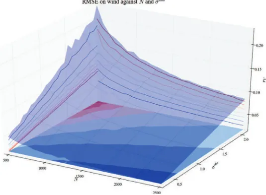
because of interactions, the 2-by-2 experiments will be fully exploited here. Three 2-by-2 experiments are required to completely visualize the influence and the interactions of these three main inputs. The figure 7.5 (respectively 7.6 ; 7.7) shows the variations of the wind RMSE when only N and σadd (repectively N and σobs ; σadd and σobs) are moving.
In the figure 7.5, one can see the wind RMSE steadily decreases with N, whatever the value of σadd. The theorem 5.1 predicts a 1/√N decrease of r
V, which look confirmed here,
independently from σadd. The effect of σaddis to increase the RMSE. But one can see that this
increase is not linear. As long as σadd< 0.5, the RMSE does not increase and then increases
rapidly (the increasing speed depends on N). The 0.5 threshold is interesting because it is the nominal value of σobs.
In the figure 7.6, one can see the effect of N is the same as in figure 7.5. The effect of
σobs is interesting. It shows a minimum around the value σobs = 0.5 which corresponds to
the nominal value of σadd. It sustains that the reconstruction is performing the best when
σobs = σadd.
Figure 7.7 crosses the effects of σobsand σaddalready observed. Two areas are to consider:
Figure 7.5 – Evolution of rV when only N and σadd vary.
the RMSE and σobs makes it increase linearly. When σobs > σadd, the evolution of the wind
RMSE is much more complex. It fastly increases with σadd. The effect of σobs is in two stages:
for very small σobs the RMSE increases and reaches a maximum and then decreases up to
the point where σobs = σadd (after what it increases again, as mentioned previously). In any
case, there is a low on the line σobs= σadd.
The best choice for σobs is thus to be equal to σadd. We have seen this can be obtained
quite safely by the tuning with the wind spectrum slope. Once this setting has been made, one can see the evolution of wind RMSE against σadd and N in figure 7.8. The RMSE increases
linearly with the observation noise and decreases as 1/√N , as the regressions in figure 7.9
show. Hence the wind RMSE can be approached by the relation (7.6) when the input σobs is
correctly set.
rV = K
σadd
√
N (7.6)
The constant K is estimated by ordinary least squares on the points of the surface 7.8 The resulting value is K = 2.33. One can see in the figure 7.9 that the wind RMSE is always lower that the input σadd, even for very low N. For example, if one has a lidar making a
error σadd = 1.19 m·s−1 (middle line in figure 7.9), the error on the wind at the output of the filter is below 0.2 m·s−1, even with only 500 particles. It reduces the noise about 83% for the lowest N tested and rate raises up to 93% with N = 2500. It shows the efficiency of the wind retrieval with the reconstruction. Even for an instrument quite noisy, the filter lessens strongly the inaccuracy on the wind.
Figure 7.6 – Evolution of rV when only N and σobs vary.
Figure 7.8 – Well set case: evolution of rV when only N and σobs vary with σobs = σadd.
Figure 7.9 – Evolution of rV with N when σobs = σadd. Regressions (dashed lines) show the
7.2.3 Effect of N on the execution time
The number of particles is the only parameter to have an influence on the execution time
Texe. The 2-by-2 experiments confirm this claim (see the results for Texe in the appendix,
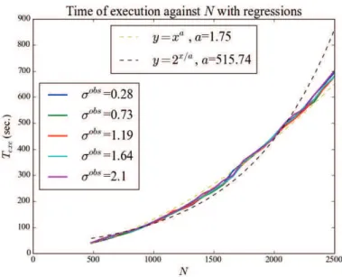
page 361). By regression, as shown in the figure 7.10, the rate of increase seems to be a power law:
Texe= Na (7.7)
The parameter a is estimated by ordinary least squares is a = 1.75. According to this relation, twice the number of particles multiply by 3.36 the execution time. The other regression tested is exponential (Texe = 2N/a), but it seems less in agreement with the observations.
Nevertheless, according to the exponential relationship, the time of execution should double each 515 particles. They are key figures to dimension numerical experiments.
Figure 7.10 – Evolution of Texe with N for different values of σobs. Regressions (dashed lines)
show the best fit is a power function.
7.2.4 Tuning strategy for the reconstruction
The best wind retrieval is thus obtained with the following three inputs values: • σadd the smallest,
• σobs equal to σadd, • N the highest.
Although σadd is fixed by the instrument, this result helps to assess which precision is
afford-able for a given instrument. Even for inaccurate instrument, the resulting error is much lower 212
than the raw error. The number of particles is bounded by the affordable time of execution. Examining these results, the following tuning strategy seems to be the most appropriate:
1. Set N to a low value, such that Texe is really small.
2. For σobs ranging around the a priori accuracy of the instrument, calculate the wind
spectrum slope b.
3. Set σobs to the value which gives b the closest to -5/3. σobs is then almost equal to σadd.
4. Set N to the maximum affordable value. The error on wind retrieval is now minimum, estimated by Kσobs
√
7.3 Other interesting results
7.3.1 On the bad construction of the score rk
After the sensitivity analysis, the output rk (TKE RMSE) have been shown to have very
complicated behaviour, including high order interactions. As a consequence, it cannot be used to tune the output. We will see at the examination of the 2-by-2 experiments that the interpretation of the score rk itself is also complex, which makes it an irrelevant score.
Figure 7.11 depicts the surface response when only ℓ and σadd vary. σadd is the most
influential input. Although its interaction with ℓ does not have a high Sobol index, one can see in the figure 7.11 that they are clearly interacting. The effect of σadddepends on the value
of ℓ. The shape of the response surface is complex and no clear interpretation can explain it. When ℓ is large, the local average is no longer local and converges to a spatial average. When ℓ is large, the RMSE rk reaches a minimum when σadd= 0.9. The value of σadd where
this minimum is reached increases when ℓ decreases. One of the unclear interpretations about this could be that RMSE on TKE is the lowest when the instrument has a variance of error comparable to the ambient turbulence. This could be checked by changing the reference wind in the system, but it has not been done here. The effect of ℓ is due to the local average used to compute the TKE. By using another TKE estimator, for example the STKE defined in the section 1.4, one should retrie the same evolution as ℓ is maximum.
Figure 7.11 – Evolution of rk when only ℓ and σadd vary.
Figure 7.12 is the response surface when only N and τ vary. Both have quite small Sobol 214
indices, but τ showed an asymmetric influence on the cobweb plot 6.25. In the figure 7.12 one can see that τ does have an influence, while N has no influence at all. The non influence of N is retrieved in the others 2-by-2 experiments in the appendix. The weird effect of τ is confirmed as well by others 2-by-2 experiments in the appendix. This effect is due to the construction of the score rk. The time average operator introduce some threshold effect that
is visible here. This effect makes difficult the interpretation of the score.
Figure 7.12 – Evolution of rk when only N and τ vary.
Finally, the figure 7.13 shows the response surface rkagainst σaddand σobs. rkis minimum
when σadd= 1.6 and σobs is not too small. When σobs is not too small, this minimum
disap-pears. There is no low on the line σobs = σadd, as for the wind RMSE. It tells that knowing
perfectly the instrument error does not help to improve rk. Whatever, is the guess of the
instrument error σobs, if the real σadd is not at the good value (related to ℓ as seen in 7.11
and probably related to the ambient turbulence), the TKE retrieval will not work. This is a very bad issue for this score because it depends on arbitrary parameters (ℓ) or uncontrollable (ambient turbulence) or unknown (if the previous reasoning are wrong). In any case, this output is hardly useful in practice.
The 2-by-2 experiments give more insight about the variations of rk. But they are complex
and there is no satisfying interpretations for them. Unverified interpretations could be that the score rk depends on the balance between the instrument error σadd and the ambient
turbulence, and not on the balance between σadd and its guess σobs. Hence, the conclusion
of this analysis is that the score rk is not well constructed and is not very informative about
Figure 7.13 – Evolution of rk when only σadd and σobs vary.
7.3.2 Influence of C0 and C1
The inputs C0 and C1 have been put in the second group of influence in the last chapter. They have a notable influence but the interaction share was the argument to put them out of the first group. Another argument was that turbulence modelling provide estimation of them. In particular, Pope (1994) proposes the relationship C1 = 12 +34C0 with the value C0 = 2.1. Nevertheless, the 2-by-2 experiments can give more insight about their influence and check if such relationship is visible in the outputs.
On the output b (wind spectrum slope) they were mentioned to be influential. Figure 7.14 shows the evolution of b when only C0 and C1 vary. One can see the response surface crosses the -5/3 value around the thick line, which has for equation C1 = 12C0. The dashed line has the equation suggested by Pope C1 = 12 +34C0. The black dot is where the nominal values have been chosen. The equation suggested by Pope looks wrong in this figure because it has been designed for 3D flows while this one is only 1D. The nominal values are close to optimal line.
On the output NG0 (number of null potential), C0 and C1 were spot as influential
(re-spectively second and third total Sobol index in figure 6.3). In the figure 7.15 is displayed the evolution of NG0 against C0 and C1. Although the sensitivity analysis let think that NG0
has complex variations when C0and C1 vary (because of interactions), the response surface is 216
Figure 7.14 – Evolution of wind spectrum slope when only C0 and C1 vary. The black dotted line are the points where C1 = 12C0. The dashed line has for equation C1 = 12 + 34C0. The dot denote the nominal values.
very smooth. One can see that a range of values are admissible (they give no null potential) and another is not. The same lines as in the previous figures are plotted (C1 = 12 + 34C0, Pope’s result, is the dashed line ; C1 = 12C0, the convenient equation for the wind spectrum, is solid dotted). The line that was admissible for the wind spectrum (C1 = 12C0, solid dotted)
is admissible here too. The line given by Pope for 3D flows (C1 = 12 +34C0, dashed) is not very convenient according to this score neither. The nominal values (C0 = 2.1, C1 = 0.9) are in the admissible area too, close to the dotted line.
On the output rV (wind RMSE), they are also in good position in figure 6.21. The figure
7.16 displays the evolution of wind RMSE when only C0 and C1 vary. The same lines as in the two previous figures are plotted. As for the two previous figures, the line C1 = 12C0 is admissible (it gives low RMSE) while the line C1 = 12 + 34C0 is not. The results are thus consistent among the 3 exploitable outputs. One more thing about the figure 7.16: it shows the extreme value C1 = 0 always gives the lowest RMSE, which is strange, because it suggests the model is better without the fluctuation term.
On the output rk the inputs C0 and C1 have a contrary effect, as shows the figure 7.17.
The line C1 = 12C0 gives the highest TKE RMSE, while the line C1 = 12 +34C0 gives lower values (still not minimum). The influence of C0 and C1 on rk is antagonist to the influence
on rV. But the sensitivity analysis raised many questions on the reliability of the score rk. It
Figure 7.15 – Evolution of NG0 when only C0 and C1 vary. The black dotted line are the
points where C1 = 12C0. The dashed line has for equation C1 = 12+34C0. The bullet denotes
the nominal values.
to C0 and C1 is not as broad as other inputs can give. Hence, to set C0 and C1, the choice is made to choose the effect on rV rather than the effect on rk.
Further examination of the influence of parameters C0 and C1 with 2-by-2 experiments confirm the influence that was suspected with Sobol indices. The response surfaces are smoother than what was expected according the interactions in which they are involved. The wind spectrum gives the sharpest criterion to choose C0 and C1. By visual examination, the relation C1 = 12C0should be fulfilled to have a -5/3 spectrum slope. This criterion is valid for the output NG0 and rV too. However, it appears to be the worst choice for the output
rk. But this output suffers from many weakness in its construction. Hence, the effect of rk
is ignored. Thus, the 2-by-2 experiment concludes that C0 and C1 must fulfil the relation
C1 = 12C0 to be well set. The nominal point (C0 = 2.1, C1 = 0.9) does not fulfil exactly, it should be improved easily.
Figure 7.16 – Evolution of wind RMSE when only C0 and C1 vary. The black dotted line are the points where C1 = 12C0. The dashed line has for equation C1 = 12 +34C0. The bullet denotes the nominal values.
Figure 7.17 – Evolution of TKE RMSE when only C0 and C1 vary. The black dotted line are the points where C1 = 12C0. The dashed line has for equation C1 = 12 +34C0. The bullet denotes the nominal values.
7.3.3 Retrieval of known variations of NG0
Figure 7.18 – Evolution of NG0 when only N and σadd vary.
The influence of N, although not visible in the Sobol indices (both in figures 6.3 and 6.41), is quite clear in figures 7.18 and 7.19. It shows a regular decrease of NG0 as N is rising. We
retrieve the behaviour predicted by the theorem 5.2 which states an exponential decrease of
NG0 with N.
The influence of σadd and σobs is described by the theorem 5.3. This theorem gives an
upper bound for the average number of null potential. This upper bound is displayed in figure 7.21. One can see this bound is very low in a large corner of the figure. The actual number of null potential, obtained when only σadd and σobs vary, is displayed in figure 7.20. One can
Figure 7.19 – Evolution of NG0 with N. Regressions show an exponential decrease.
Figure 7.20 – Evolution of NG0 when only
σadd and σobs vary. Figure 7.21 – Theoretical average for the Noutput against σadd and σobs. G0
7.4 Conclusion
So-called 2-by-2 experiments are the computation of the surface response when only 2 inputs vary and the others are kept to their nominal values. It allows visualizations of the surface response which are not possible in higher dimensions and thus help to find the shape of the response function f. Such visualizations have been used to confirm the tuning strategy coming out of the sensitivity analysis. Only few 2-by-2 experiments are necessary, thanks to the ranking of importance made by the sensitivity analysis. The surface response of wind spectrum slope and wind RMSE have been commented and confirm the following tuning strategy:
1. Set N to a low value, such that Texe is really small.
2. For σobs ranging around the a priori accuracy of the instrument, calculate the wind
spectrum slope b.
3. Set σobs to the value which gives b the closest to -5/3. σobs is then almost equal to σadd.
4. Set N to the maximum affordable value. The error on wind retrieval is now minimum, estimated by Kσobs
√
N with K = 2.33.
Beside, some results of the 2-by-2 experiments have been used to check remarkable points. From these additional examinations, it comes out that
• The score rk has been shown to be not very well constructed because it is not very
informative on the system.
• The inputs C0 and C1 have been left apart from the tuning strategy, they are explored with 2-by-2 experiments. It yields that the setting fulfilling the relation C1= 12C0 gives the best results.
• The influence of N on NG0 is in agreement with the theorem 5.2, although not visible
in the Sobol indices.
The full results of 2-by-2 experiments have not been commented all, but they are let available to the curious reader in the appendix C, page 301.
Chapter 8
Penalised regression to estimate the
Sobol indices
Contents
8.1 Sobol indices estimated by regression . . . 225
8.1.1 Motivation . . . 225 8.1.2 Linear model statement . . . 226
8.2 Properties and links among estimators . . . 228
8.2.1 The least squares estimator . . . 229 8.2.2 Lasso versus least square . . . 230 8.2.3 Best subset versus least square . . . 231 8.2.4 Lasso versus best subset . . . 232
8.3 Choice of penalty by cross-validation . . . 234
8.3.1 General principle of cross-validation . . . 234 8.3.2 Uncertainty of prediction and uncertainty of estimation . . . 235 8.3.3 Application to Sobol indices estimation . . . 236 8.3.4 Results of numerical experiments . . . 237
8.4 Conclusion . . . 241
8.1 Sobol indices estimated by regression
8.1.1 Motivation
In the chapter 4, several estimators for Sobol indices have been presented. They are all based on a different way to estimate the average operator in the Sobol index. For example, Sobol (2001) compares 2 estimators (though denoted λ and µ in the paper, here the notations of the previous chapter are kept):
ä Du M C1 = 1 N N Ø i=1 f (Xi)f (Zui, Xui¯)− A 1 N N Ø i=1 f (Xi) B2 (8.1)
ä Du M C2 = 1 N N Ø i=1 1 f (Xi)− f(Zui, Xui¯)22 (8.2) He shows that äDu M C2
has a smaller variance to estimate total Sobol indices, while äDu
M C1
has a smaller variance to estimate main effect Sobol indices. Moreover, äDu
M C2
is always positive, which avoid the estimation to be negative when indices are small. Saltelli et al. (2010) makes a broader comparison focused on the estimation of first order Sobol indices, and proposes another Monte Carlo estimator:
ä Du M C3 = 1 N N Ø i=1 f (Xi)1f (Zi)− f(Zui, Xu¯i) 2 (8.3) Owen (2013) also makes a comparison of several estimation strategies and proposes a new estimator with the concern of improving the estimation of small Sobol indices.
Among all these estimators, the estimation method of V (E [Y |Xu]) is modified to improve
its efficiency (smaller variance, more efficient calculation) or to retrieve valuable properties (positivity, asymptotic normality). In this section, we present another type of estimation, based on a linear regression. When sensitivity analysis comes to the user, a complete set of Sobol indices is not always informative. The interpretation of the highlighted sensitivity is the final result of the sensitivity analysis. Only few coefficients are relevant to describe the contribution of variance. Poorly influential groups are not taken into account in the interpretation of the Sobol indices, even though their Sobol index is not exactly zero. Using a linear regression opens to all feature selection techniques and makes the final result easier to interpret. It also gives an alternative way to get estimators with good properties. In addition, the optimisation formulation of regression takes profit of many efficient off-the-shelves algorithms to make the minimization. Three estimators are presented and compared:
• The least squares estimator : Sãu
ls
• The Lasso estimator : Sãu
l1
• The best subset estimator : Sãu
l0
First, the Sobol index estimation with regression is stated in a general way. Then, the prop-erties and the relationship among the three considered estimators are reviewed. A strategy to set the penalty is also given. Next, a small scale numerical experiment is carried out on the case of turbulent medium reconstruction.
8.1.2 Linear model statement
The notation will be the same as in the chapter 4: 226
• [[1, p]] = {1, . . . , p}
• I is the collection of all subset of [[1, p]] (thus of cardinal 2p).
• u is an element of I.
• | · | the cardinal of the set "·". For example, |u| is the number of indices in u ; and |I| is the number of groups of indices in I (|I| = 2p).
• I′ ⊂ I is the number of subsets considered. d = |I′| 6 2p is its cardinal. For example,
if one is interested in first and second order Sobol indices only, one will have I′ = [[1, p]]∪ {(i, j) ∈ [[1, p]]2}.
• For all u ∈ I, it is denoted ¯u = [[1, p]] \ u = {i ∈ [[1, p]], i /∈ u}
• X = (X1, ..., Xp) is the vector of random inputs (inputs are assumed independent).
• Z = (Z1, ..., Zp) is an independent copy of X.
• Y = f(X) = (X1, ..., Xp) is the output (also random).
• Xu= (Xi)i∈u is the vector of random inputs in u. • Zu = (Zi)i∈u is an independent copy of Xu.
• Yu= f (Zu, Xu¯) is the output when the inputs in u are taken from another independent realisation.
The aim is to estimate Su =
cov(Y,Yu)
V(Y ) . It is the coefficient of the slope of the linear
regression between Y and Yu:
Lemme 8.1. For any set u of indices (u ∈ I′), when (au, bu) = arg min (a,b) î Eè(Y − aYu− b)2é+ Eè(Y u− aY − b)2 éï (8.4) then au= Su
Proof is in the appendix B.3.1.
The lemma 8.1 shows the best coefficient to predict the total variance from the predictor
Yu is the Sobol index Su. The coefficient au in the linear model of the lemma is equal to the
Sobol index even if E [Y ] Ó= 0. The bu coefficient is not interesting to interpret the variance.
Hence, in the following, we will suppose that the output Y is centred: E [Y ] = 0. The variance of the output can be explained with the linear model (8.5).
The statistical model (8.5) answers the following question: if the output Y has to be explained with Yu(the same code with the input parameters Xufrozen), how much variance is it possible
to explain? The best approximation of Y as a function of Yuis E [Y |Yu] (it can be seen as the
projection of Y onto Yu). The assumption stated by the linear model is that E [Y |Yu] = auYu.
As a consequence, the error ǫ of such model is a centred and the coefficient au is chosen to
minimize its variance. The variance of ǫu when it is minimum is denoted σ0u2 .
The statistical model (8.5) can be used to estimate only the Sobol index Su. The aim is to
get all Sobol indices at once. The vector of all slopes is denoted a = (au, u∈ I′). The vector
of all Sobol indices is denoted S = (Su, u ∈ I′). These vectors are of dimension d = |I′|.
Finally, the minimization problem (8.4) is changed into (8.6). Sls= arg min a Ø u∈I′ Eè(Y − auYu)2é+ Eè(Y u− auY )2 é (8.6)
The minimization of (8.6) benefits then from the advances in linear regression. In partic-ular, we will focus on two penalties to select the most relevant coefficients: the L1 penalty (problem 8.7, Lasso method) and the L0 penalty (problem 8.8, best subset method).
Sl1 = arg min a Ø u∈I′ Eè(Y − auYu)2é+ Eè(Y u− auY )2 é + λëaë1 (8.7)
with the L1 norm ëaë1 =q
u∈I′|au|. Sl0 = arg min a Ø u∈I′ Eè(Y − auYu)2é+ Eè(Y u− auY )2 é + λëaë0 (8.8)
with the L0 norm ëaë0 =q
u∈I′1auÓ=0 =|{u, auÓ= 0}|.
8.2 Properties and links among estimators
The theoretical Sobol indices from penalized regression have been defined: least squares (8.6), Lasso (8.7), best subset (8.8). Now we focus on their estimation. The problem is to find an estimation of the coefficients in the linear model (8.5) from the following data:
Y = y1 ... yN Yu = yu1 ... yN u for all u ∈ I′. The samples Y and Y
u are denoted the same way as the random variables Y
and Yu they are sampling.
Moreover, the random variables Y and Yu are assumed centred: E [Y ] = E [Yu] = 0 which
has for consequenceqN
i=1yi=qNi=1yui = 0. Since the random variables Y and Yu follow the
same law, we have E#Y2$ = E#Yu2$ = σ2 and so qNi=1(yi)2 = qNi=1(yui)2 = ˆσ2 ≃ σ2. The variance of the noise in the linear model (8.5) is denoted σ2
0u = V (Y − auYu).
8.2.1 The least squares estimator
The coefficients of the linear model (8.5) can be estimated with ordinary least squares. The problem to solve in theory (8.6). In estimation, it is (8.9):
â Sls= arg min a Ø u∈I′ ëY − auYuë22+ëYu− auYë22 (8.9)
For any u ∈ I′, the solution is given by (8.10): â Suls= (YuTYu)−1YuTY = qN i=1yiyiu qN i=1(yiu)2 (8.10) The least squares estimator is known to be the BLUE: Best Linear Unbiased Estimator. Its bias is zero and its variance is minimum among all estimators of the form AY with A ∈ Rd×N (Gauss-Markov theorem, (Saporta, 2006) section 17.2).
EèSâulsé= Su (8.11) V1Sâuls|Yu 2 = (YuTYu)−1σ20 = σ02 σ2 (8.12)
Its expression is the same as the Monte Carlo estimator Däu
M C1
. Janon et al. (2014) already pointed out the equality of such estimators (remark 1.3 of the paper) and they proved their asymptotic normality (proposition 2.2 of the paper). Moreover, the asymptotic variance of the estimator given by Janon (denoted σ2
M C1) and the variance given by Gauss-Markov theorem
(equation (8.12)) are the same. Indeed, when Y is centred, σ2
M C1 is written
σ2M C1 = V (Y (Yu− SuY ))
V (Y )2 From Janon et al. (2014)
= V (Yu− SuY )
V (Y ) because E [Yu− SuY ] = E [Y ] = 0 and (Yu, Y ) = (Y, Yu)
= σ
2 0
σ2
In conclusion, the least squares method gives the same estimator as crude Monte Carlo. This estimator is unbiased but asymptotically Gaussian: if the samples Y and Yu are too
8.2.2 Lasso versus least square
The Lasso method (Least Absolute Shrinkage and Selection Operator) aims to solve a least squares problem while pushing some coefficients to be exactly 0. It is thus a valuable tool when the vector of coefficient is sparse (van de Geer, 2016). Having several coefficients equal to zero makes the statistical model more informative and more easily interpreted: predictors with a coefficient to 0 are dismissed. The Lasso method was first introduced by Tibshirani (1996). The principle is to solve the least square problem with a L1-penalty in the function to minimize.
The use of a L1-penalty is what make some coefficients to be exactly zero. Indeed, the admissible area has a very different shape with the L1norm and the L2norm. This is visible in the figure 8.1: an illustration with p = 2 is presented. On the right hand side, the admissible area for the L2norm is a circle. On the left hand side, the admissible area for the L1norm is a square with angle on the axis. The solution of the unconstrained problem (8.6) is denotedβâLS
in the figure 8.1 and the lines of equal cost are drawn in red. The solution of the constrained problem is the point in the admissible area the closest to βâLS according to the cost lines in red. For the L2 norm (right panel), the solution is on a circle. Both coefficients are likely to be non-zero. For the L1 norm (left panel), the solution is likely on one of the corner of the square. On any corner, one the coefficient will be exactly zero.
Figure 8.1 – Illustration of admissible area with L1 and L2 norms. The extreme points are located on an axis for the L1 norm, thus one of the coefficient is null.
Credit: Par LaBaguette — Travail personnel, CC BY-SA 4.0,
https://commons.wikimedia.org/w/index.php?curid=48816401
The Lasso is written only for the Sobol indices estimation problem. The problem to solve 230
is (8.13) and the solution is given by the proposition (8.1). â Sl1= arg min a Ø u∈I′
ëY − auYuë22+ëYu− auYë22+ λ1ëaë1
(8.13)
Proposition 8.1. For any u ∈ I′, the Lasso and least squares estimators are related according
to the following formula:
â
Sul1= max1Sâuls− ε1, 02 with ε1= 2σλ12.
Proof is in the appendix B.3.2, page 296.
The Lasso method gives an estimator that has a direct relationship with the least squares estimator. To get the Lasso estimator, the least square estimator is shrunk of ε1 = λ1/(2σ2). When the least squares estimator is smaller that the shrunk, the Lasso estimator is exactly zero.
From a Bayesian point of view, the penalty is equivalent to give a prior distribution to the coefficients a. The L1-penalty imposes an absolute exponential prior distribution: ∀a ∈ a, P (a) ∝ exp(−λ1|a|). Maximizing the likelihood gives the least squares estimator. Maximizing the posterior probability with an absolute exponential prior gives the Lasso esti-mator.
The hard part to take profit of the Lasso is to correctly set the penalty λ1. When λ1 → 0, the estimator tends to the ordinary least squares estimator and there is no benefit to use the Lasso. When λ1→ +∞, the penalty unrealistically shrinks the coefficients to estimate. Good predictors will be dismissed, leading to too simple models.
8.2.3 Best subset versus least square
The so-called best subset method (mentioned in (Tibshirani, 1996; Breiman, 1995; Lin et al., 2010)) adds a L0 penalty to the least square problem (equation (8.8)):
â Sl0= arg min a Ø u∈I′
ëY − auYuë22+ëYu− auYë22+ λ0ëaë0 with the L0 norm ëaë0 =|{i, a
Proposition 8.2. For any u ∈ I′, the best subset and least squares estimators are related
according to the following formula:
â Sul0 =Sâuls1Sâls u>ε0 with ε0= ñ λ0 σ2.
Proof is in the appendix B.3.3, page 298.
The best subset estimator gives also an estimator directly linked with the least square estimator. When the least square estimator is smaller than the threshold ε0 =√λ0/σ, the best subset estimator is exactly zero. Otherwise, least square and best subset estimators are equal. The shrinkage is not systematic, conversely to the Lasso. As for the Lasso, the difficulty is to correctly choose the penalty λ0.
The best subset estimator is optimal in terms of information loss. Indeed, it minimizes the Akaike information criterion. The Akaike information criterion (AIC) is a metric of the information loss due to the model (original publication in 1973, republished in the collection (Akaike, 1998)). The model Y = auYu+ ǫu is imperfect and the AIC quantifies the benefit
of adding a new predictor. It is defined by
AIC = 2k− 2 log(L(a))
where k is the number of coefficients to estimate and L is the likelihood function. In our case,
k is the number of non-zero Sobol indices and the likelihood function is given by
log(L(a)) = log(P (Y|a)) ∝Ø
u∈I
ëY − auYuë22
Hence, the AIC for our problem is exactly the function of a to minimize in the best subset problem (8.8).
Unfortunately, the minimization with a L0 penalty is a NP-hard problem (Natarajan, 1995). As a consequence, only greedy algorithms can perform the minimisation of (8.8). For example, in (Tibshirani, 1996), they are estimated using the so-called leaps and bounds procedure (Furnival and Wilson, 1974).
8.2.4 Lasso versus best subset
Lasso and best subset estimators are both related to the least squares estimator. Transitively, they are related to each other. The property 8.1 tells the Lasso is soft threshold of the least square estimator, while property 8.2 tells the best subset is a hard threshold of the least square estimator. The threshold of Lasso is said soft because it is continuous, while the hard threshold is not. Shapes of both threshold functions are displayed in figures (8.2) and (8.3).
Figure 8.2 – Soft threshold: link between the Lasso estimator and the least square estima-tor.
Figure 8.3 – Hard threshold: link between the best subset estimator and the least square estimator.
To have the same threshold ε = ε1 = ε0, we need to have the following relation between the penalty:
λ1 = 2σ ð
λ0 (8.14)
In this case, the relationship between Sâl0
u and Sâul1 is easy to write and valid everywhere but
at the discontinuity (when Sâuls= ε). â Sul0= Sâ ls u â Sls u − ε â Sul1 (8.15)
When the thresholds are different, one need to distinguish the case ε1 < ε0 and ε1 > ε0 and then the sub-cases Sâuls < min(ε1, ε0), Sâuls ∈]ε1, ε0[ and Sâuls > max(ε1, ε0). The final result does not feed the comment. One can see that Sâl0
u → Sâul1 either when ε → 0 (both converge
toward Sâuls when the penalty decreases) either whenSâuls→ +∞. It highlights that the use of
L1 or L0 penalty is only relevant for small Sobol indices. For large Sobol indices,Sâuls has the
advantage to be unbiased.
Even with an expression of Sâul0 and Sâul1 as a function of Sâuls, for which the asymptotic
behaviour is known, the asymptotic law of the penalized estimators are not straightforward. The Delta method does not apply because neither soft nor hard threshold functions are differentiable.
Lin et al. (2010, 2008) argue in favour of the L0penalty. They compare L1and L0penalties according to the predictive risk function R(β,β) = Eâ èëXβ − Xβâë22é and show that the risk
ratio of L0 over L1 is bounded while the risk ratio of L1 over L0 is not. The final estimate of L0 is better, but the algorithm to get it are not efficient. Indeed, Natarajan (1995) proved that the L0-penalized least squares is a NP-hard problem. Hence, even if the L0 estimate is better, more efficient algorithms exist for the L1 estimate.
8.3 Choice of penalty by cross-validation
8.3.1 General principle of cross-validation
Given a linear model Y = Xβ + ǫ, one wants to estimate β and the uncertainty on the estimation. The principle of cross-validation is to split the sample X in two part: a part dedicated to the estimation of the coefficient in the regression, another part dedicated to the prediction of the model with the estimated sample. On the part dedicated to the prediction, one has both the reference value (given in the sample) and the predicted value. Hence, one can have a score of error on the model.
The sample (Y, X) where Y ∈ RN and X ∈ RN×d is divided into one sample (Y
A, A) used
for the estimation of the coefficient (the training sample), and a sample (YB, B) used for the
prediction and error estimation (the testing sample). We denote NA the size of the learning
sample.
The training phase provides the estimated coefficients β in the linear model Y = βX + ǫ.â The regression (with or without penalty) is performed on the sample (YA, A). For instance,
for the ordinary least squares, we have the formula â
β = (ATA)−1ATYA
Using this estimated coefficient, the output is predicted with the predictors of the second sample. The comparison with the observed output provides an estimation of the uncertainty of prediction:
ǫ≃ YB− Bβâ
In particular, one can check the bias, variance and mean squared error. In our case, we are interested in the uncertainty of estimation. The uncertainty of estimation has to be derived from the uncertainty of prediction.
8.3.2 Uncertainty of prediction and uncertainty of estimation
The uncertainty on prediction quantifies the error made by the model when it is applied on new data. The uncertainty on estimation quantifies the error made in the estimation by comparing to a new dataset. By splitting the sample into a training sample and a testing sample, one can access the uncertainty of prediction. But the uncertainty of estimation is not directly accessible and has to be derived from the uncertainty of prediction. If we consider a linear model Y = Xβ + ǫ, with Y ∈ R, X ∈ Rd, β ∈ Rdand we assume we have an estimation
â
β of the coefficient which is independent of X.
The uncertainty of the prediction Y = Xâ β of the variable Y is described by its bias,â
variance, and mean-squared error (MSE).
BiY = EèYâ − Yé (8.16)
VarY = V1Yâ2= Eè(Yâ − EèYâé)2é (8.17)
MSEY = Eè(Yâ − Y )2é (8.18)
These statistics describe the uncertainty of prediction. But for this application, we are more interested on the error of estimation: bias, variance and MSE for the estimated coeffi-cients β.
Biβ = Eèβâé− β (8.19)
Varβ = V1βâ2= Eè(βâ− Eèβâé)(βâ− Eèβâé)Té (8.20)
MSEβ = Eè(βâ− β)T(βâ− β)é (8.21)
Note that they all are of different dimensions: Biβ ∈ Rd, Varβ ∈ Rd×d and MSEβ ∈ R.
Although, they are linked by the following relation:
MSEβ = BiTβBiβ + tr(Varβ) (8.22)
where tr(·) is the trace operator.
The uncertainty of prediction and estimation are linked with the following relations when â β is independent from X: BiY = E [X] Biβ (8.23) VarY = EèXVarβXTé+ V1XEèβâé2 (8.24) MSEY = BiT βE è XTXéBiβ+ Eètr(XVarβXT)é+ σ2 0 (8.25)
Proof is in the appendix B.3.4.
In the case of the Lasso method, the cross-validation is repeated for different values of penalty. As the estimator given by the ordinary least squares is unbiased, the bias of
esti-mation should decrease with the penalty. Conversely, a large penalty shrinks the coefficients and thus reduces the variance of the estimator but its bias grows. In the middle, we expect the mean squared error to reach a minimum.
lim
λ→0
Biβ(λ) = 0 and lim
λ→+∞
Varβ(λ) = 0
With the testing sample, one can estimate the bias, variance and mean squared error of prediction (equations (8.16),(8.17),(8.18)). They can be linked to the same statistics for es-timation (equations (8.19),(8.20),(8.21)) through the formulae (8.23), (8.24) and (8.25). The penalty is then chosen to minimise the error of prediction MSEY(λ). When this minimum
is reached, the chosen penalty makes a good comprise between bias and variance of estimation.
8.3.3 Application to Sobol indices estimation
For our particular problem, the linear model is not of the form Y = Xβ + ǫ. Instead, we have d linear models of the form Y = auYu+ ǫu. There is only one predictor which verifies
E [Yu] = 0 and E#Yu2
$
= σ2, for any u. The error ǫu has no reason to be the same for each
model: E [ǫu] = 0 and E#ǫ2u
$ = σ2
0u. Applying the formulae (8.23), (8.24) and (8.25) we have:
BiuY = =0 ú ýü û E [Yu]Biua = 0 (8.26) Varu Y = σ2(Varua + E [aãu]2) (8.27) MSEu
Y = σ2(Biua)2+ σ2Varua + σ0u2 = σ2MSEua+ σ20u(1− σ2) (8.28) In practice, the estimators of bias, variance and mean squared error of prediction are accessible through the formulae:
ä Biu Y = 1 N N Ø i=1 (yuiaãu− yi) (8.29) [ Varu Y = 1 N− 1 N Ø i=1 A yuiaãu− 1 N N Ø i=1 yuiaãu B2 (8.30) \ MSEu Y = 1 N N Ø i=1 (yi− yuiaãu)2 (8.31)
On the two last series of equation, one can see that the estimator for the bias is useless. Indeed, despite the link (8.23) between bias of prediction and bias of estimation, despite the fact that Bia(λ) is expected to increase with λ, the estimator (8.29) cannot be used to retrieve
that trend because of the relation (8.26).
For the variance and mean-squared error, we would rather have a score for all the coeffi-cients, not one for each u. Applying the definition of the MSE for any vector of parameters
β (equation 8.21) to the case β = a and β = (auYu+ ǫu, u∈ I′), the relevant global MSE is
the sum of MSE for each u.
MSEY = Ø u∈I′ MSEu Y and MSEa= Ø u∈I′ MSEu a tr(VarY) = Ø u∈I′ Varu Y and tr(Vara) = Ø u∈I′ Varu a Finally, tr(VarY) = σ2 tr(Vara) + Ø u∈I′ E [aãu]2 MSEY = σ2MSEa+ (1− σ2) Ø u∈I′ σ0u2
In the equation of variance, the terms E [aãu]2 vary with penalty (they are linked to the bias
which is not accessible). The variations of tr(VarY) against λ are thus not equal to the
variations of tr(Vara). In the equation of MSE, σ2 = V (Y ) is a constant, σ20u = V (ǫu) is the
minimum variance of the least squares problem. It is also a constant (it depends only on u). The variations of MSEY are the same as MSEa. Hence, the error of estimation is minimum
when the error of prediction is minimum.
In conclusion, the penalty will be chosen to minimize the error of prediction. In the par-ticular case of centred design, the bias of prediction is longer linked to the bias of estimation. The variance of prediction rely on additional terms that are still to be estimated to complete the link between prediction and estimation. As a consequence, only mean-squared error plot will be used.
8.3.4 Results of numerical experiments
The three estimators presented in the last section will be experimented on the application case of turbulence reconstruction. The sample of inputs X and Z are generated with latin hypercubes. For both X and Z, 4000 values of each input are generated. The split between samples for cross-validation have been made randomly, with a proportion of 65% for the training sample (2400 values) and 35% for the test sample (1600 values). Once the sample has been split, the random state of the splitting is saved in case the experiment is repeated in the same conditions. The experiment have been carried out with the meta-model of the output rV (the root-mean squared error on the wind) because it is easy to interpret. The
algo-rithm used to minimize the cost functions (least squares and Lasso) is the conjugated gradient. The figures (8.4) and (8.5) show the evolution of the estimated mean-squared error \MSEY of the Lasso for different penalty values. On the left (figure 8.4) the Lasso estimate have
calculated from the Monte-Carlo estimate, on which the soft-threshold function has been applied, using the proposition 8.1. On the right (figure 8.5) the Lasso estimate have calculated by the minimization of the cost function defined by (8.7) (L1 penalized least squares). One can see a clear minimum on both. Although, the slope is much more regular when the soft threshold is applied. Indeed, it avoids the weaknesses of the minimization: do not reach the exact minimum but something close enough, get stuck at a local minimum... Overall, the comparison of both figures corroborates the minimization is trustworthy. But in the objective to apply another minimum finder to such curve, the soft threshold one is recommended. Moreover, the soft threshold one is much faster to compute.
As a conclusion, to find the good penalty value by cross-validation, we recommend to do first an ordinary least squares regression on the training sample, then to get the Lasso estimate by soft thresholding for all the penalty values and eventually to compute the mean squared error on the testing sample. This recommendation holds only for problems which have a result similar to the proposition 8.1.
Figure 8.4 – Estimated mean squared error against the penalty in Lasso estimation. Ob-tained with soft thresholding of the Monte Carlo estimate.
Figure 8.5 – Estimated mean squared error against the penalty in Lasso estimation. Ob-tained with the minimization of the cost func-tion.
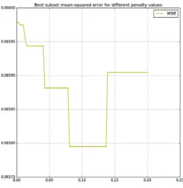
This methodology can be extended to the L0 penalty. The best subset estimator resulting from L0 penalized regression has been shown to be accessible through a hard thresholding of the least squares estimator (proposition 8.2). This was the only method of estimation tested here since only greedy algorithm can solve the L0 penalized minimization. As a consequence, the parameter to check will not be the penalty λ0 but the threshold ε0 =
ñ
λ0
σ2. The Monte
Carlo estimate is calculated on the training sample. For each threshold value, the mean squared error is estimated on the testing sample. It results the curve in figure 8.6.
One can see the step-like shape of the curve: the threshold does not have influence until it reaches the next coefficient value. As a consequence, the minimum is not unique. For this example, it is reached for a threshold around 0.1, which a large value. It let only two non-zero indices. It points out the method of selection is not perfect and might be too selective. In (Fruth et al., 2011) the value of 0.02 is used to threshold second order Sobol indices (figure 2 in the 2011 version on HAL). This value will be used here as well.
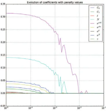
Figure 8.6 – Estimated mean squared error against the threshold in best subset estimation. The figure 8.7 shows the evolution of the coefficients with the penalty. On the x-axis is the value of the penalty in logarithmic scale. On the y-axis is the value of the estimated coefficients. One can see that for a penalty almost null, the coefficients are all non-zeros. Actually they are equal to their ordinary least squares estimate. For a very large penalty, all coefficients are null. When the penalty decreases, they raise one after another. The introduc-tion of a new coefficient can sometimes influence the curve of another coefficient. This is the sign of a correlation between them (as in (Hesterberg et al., 2008), figure 2). No such feature is visible in the figure. This is not surprising since the inputs of the sensitivity analysis have been simulated independently. Although it is good to be confirmed by this observation.
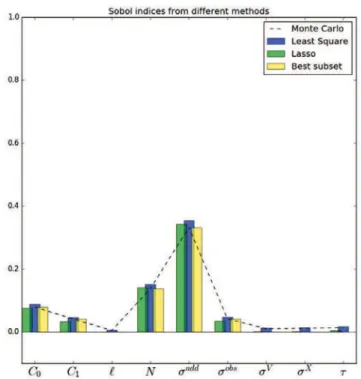
Four estimators have been tested: the straightforward Monte Carlo, the ordinary least squares, the Lasso and the best subset. They are displayed in figure (8.8). As expected, the least squares (blue) and the Monte Carlo (black dashed line) are two realisations of the same
Figure 8.7 – Value of the coefficients estimated by Lasso regression against the penalty (in log-scale). The coefficients are all at 0 for large penalty and raise in order of importance up to their value as obtained with ordinary least square.
estimator. The Lasso (green) shrinks all the coefficients up to 0. It results that only the main indices are kept non-zero and the negative estimation of small indices are filtered. The best subset (yellow) also selects the major coefficients, but it does not shrink them. The hard threshold was set to the value ε0 = 0.02.
Figure 8.8 – Three estimators ensuing from regression (coloured bars) are compared to the Monte Carlo estimator (black dashed line). One can see that the ordinary least square (blue) gives the same estimation (more or less some randomness due to estimation). The best subset is exactly equal to the Monte Carlo, excepted for indices smaller than the threshold, which are 0. The Lasso estimator gives a shrunk estimation bounded to 0.
8.4 Conclusion
Sobol indices summarize the influence of a group of parameters with a real number in [0, 1]. But the number of groups grows exponentially with the number of parameters (if the code has p parameters, there are 2p groups of parameters). In practice, only few of them are really
influencing the code. Moreover, the interpretation of the Sobol indices will focus only on the main ones. That is to say, a good estimation of Sobol indices is not necessarily an unbiased estimation.
Penalized regressions offer biased estimators with lower variance such that the total error is lower. From the initial remark that Sobol indices can be seen as the estimated parameter in a linear model, three regression types have been tested. The ordinary least squares give the same estimate as with Monte Carlo. The L1 penalized least squares give the Lasso estimate. The L0penalized least squares give the best subset estimate. The Lasso shrinks all coefficients and set the smallest ones to exactly zero. The best subset does not shrink the coefficients but set the smallest ones to exactly zero. They are linked to the least squares estimate with a soft threshold and a hard threshold, respectively.
To set the penalty objectively, a cross-validation has been carried out for each penalty value in a given set. The penalty which gives the lowest mean squared error is chosen to
perform the final estimation. The application of this methodology on a single example has shown good results, but more experimentations are needed to assess if it can be repeated and trusted.