RESEARCH OUTPUTS / RÉSULTATS DE RECHERCHE
Author(s) - Auteur(s) :
Publication date - Date de publication :
Permanent link - Permalien :
Rights / License - Licence de droit d’auteur :
Dépôt Institutionnel - Portail de la Recherche
researchportal.unamur.be
University of Namur
High-resolution gridded population datasets for Latin America and the Caribbean in
2010, 2015, and 2020
Sorichetta, Alessandro; Hornby, Graeme M; Stevens, Forrest R; Gaughan, Andrea E; Linard,
Catherine; Tatem, Andrew J
Published in:
Journal on Data Semantics DOI:
10.1038/sdata.2015.45
Publication date: 2015
Document Version
Publisher's PDF, also known as Version of record
Link to publication
Citation for pulished version (HARVARD):
Sorichetta, A, Hornby, GM, Stevens, FR, Gaughan, AE, Linard, C & Tatem, AJ 2015, 'High-resolution gridded population datasets for Latin America and the Caribbean in 2010, 2015, and 2020', Journal on Data Semantics, vol. 2, pp. 150045. https://doi.org/10.1038/sdata.2015.45
General rights
Copyright and moral rights for the publications made accessible in the public portal are retained by the authors and/or other copyright owners and it is a condition of accessing publications that users recognise and abide by the legal requirements associated with these rights. • Users may download and print one copy of any publication from the public portal for the purpose of private study or research. • You may not further distribute the material or use it for any profit-making activity or commercial gain
• You may freely distribute the URL identifying the publication in the public portal ?
Take down policy
If you believe that this document breaches copyright please contact us providing details, and we will remove access to the work immediately and investigate your claim.
High-resolution gridded population
datasets for Latin America and the
Caribbean in 2010, 2015, and 2020
Alessandro Sorichetta1,2, Graeme M. Hornby3, Forrest R. Stevens4, Andrea E. Gaughan4, Catherine Linard5,6& Andrew J. Tatem1,7,8
The Latin America and the Caribbean region is one of the most urbanized regions in the world, with a total population of around 630 million that is expected to increase by 25% by 2050. In this context, detailed and contemporary datasets accurately describing the distribution of residential population in the region are required for measuring the impacts of population growth, monitoring changes, supporting environmental and health applications, and planning interventions. To support these needs, an open access archive of high-resolution gridded population datasets was created through disaggregation of the most recent official population count data available for 28 countries located in the region. These datasets are described here along with the approach and methods used to create and validate them. For each country, population distribution datasets, having a resolution of 3 arc seconds (approximately 100 m at the equator), were produced for the population count year, as well as for 2010, 2015, and 2020. All these products are available both through the WorldPop Project website and the WorldPop Dataverse Repository.
Design Type(s) data integration objective • database creation objective • time series design Measurement Type(s) population
Technology Type(s) census Factor Type(s)
Sample Characteristic(s)
Homo sapiens • Antigua and Barbuda • anthropogenic habitat • Argentina
• Belize • Bolivia • Brazil • Chile • Colombia • Costa Rica • Cuba •
Dominican Republic • Ecuador • El Salvador • French Guiana Region •
Guatemala • Guyana • Haiti • Honduras • Jamaica • Mexico •
Nicaragua • Panama • Paraguay • Peru • Puerto Rico • Suriname • Trinidad and Tobago • Uruguay • Venezuela
1Geography and Environment, University of Southampton, Highfield Campus, Southampton SO17 1BJ, UK. 2Institute for Life Sciences, University of Southampton, Highfield Campus, Southampton SO17 1BJ, UK.3GeoData, University of Southampton, Highfield Campus, Southampton SO17 1BJ, UK. 4Department of Geography and Geosciences, University of Louisville, Louisville, KY 40292, USA.5Lutte biologique et Ecologie spatiale (LUBIES), Université Libre de Bruxelles, CP 160/12, 50 Avenue F.D. Roosevelt, Bruxelles B-1050, Belgium.6Fonds National de la Recherche Scientifique, 5 rue d'Egmont, Bruxelles B-1000, Belgium. 7Fogarty International Center, National Institutes of Health, 16 Center Drive, Bethesda, MD 20892, USA. 8Flowminder Foundation, Roslagsgatan 17 SE-11355, Stockholm, Sweden. Correspondence and requests for materials should be addressed to A.S. (email: [email protected]).
OPEN
SUBJECT CATEGORIES » Geography » Malaria » Sustainability » Environmental sciences Received: 16 June 2015 Accepted: 07 August 2015 Published: 01 September 2015Background & Summary
The Latin America and the Caribbean region has a population of around 630 million and is one of the most urbanized regions in the world, with 80% of its population currently living in urban areas. Its population, which increased by 1.5 times over the last 25 years, is expected to grow by another 25% and further urbanize by 2050, with 86% living in urban areas1.
According to the Pan American Health Organization2, health and demographic indicators highlight that, although with significant variation from country to country and to a far lower degree than Africa and central Asia, the region is characterized by relatively high maternal and infant mortality rates, and a lack of access to health facilities and services for a large part of its population. In addition, many endemic infectious diseases are also present and include malaria, dengue, chikungunya, chagas, and leishmaniasis3,4. Furthermore, low and middle income countries located in the region are highly vulnerable to and affected by natural and man-made disasters5and, according to the Fifth Assessment Report of the Intergovernmental Panel on Climate Change6, the frequency and intensity of weather- and water-related hazards are expected to rise in the upcoming decades, both globally and regionally, as a consequence of climate change. Finally, the rapid development of the region and its ongoing urbanization is expected to further exacerbate problems related to the rapid land-use change and deforestation in rural areas7and the growth of informal settlements in urban areas8.
In this context, contemporary, spatially detailed, and comparable datasets that accurately depict the distribution of the residential human population are a fundamental prerequisite for measuring the impacts of population growth9, monitoring changes10, supporting environmental and health applications11,12, and planning interventions13. Nevertheless, for the majority of these countries, and especially for those most severely and disproportionately affected by both natural disaster and infectious disease morbidity, contemporary, spatially detailed, consistent, and open data on population distribution are often unavailable or difficult to obtain.
For these reasons, since the mid-1990s, there has been an increasing effort to create spatially-explicit population datasets by using a range of approaches, assumptions, and input data to disaggregate administrative unit-based population counts to a regular grid of fixed spatial resolution14. Current global gridded datasets depicting the distribution of human population across the Latin America and the Caribbean region include various versions of the Gridded Population of the World (GPW)15–18, the Global Rural-Urban Mapping Project (GRUMP)19, the Oak Ridge National Laboratory's LandScan20, and the United Nation Environment Programme Latin American and Caribbean Population Database21. However, these datasets present certain limitations due to their spatial resolution ranging between 30 and 150 arc seconds (approximately 1 and 5 km at the equator, respectively), the age and coarse spatial detail of the input population count data, or the lack of details on the input data and modelling approach used to produce them22,23.
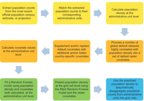
In the framework of the WorldPop Project (www.worldpop.org), an open access archive of high-resolution gridded population distribution datasets for the Latin America and the Caribbean region has been created using the most recent and finest level census and official population estimate data available at the time of writing, along with a range of ancillary geospatial datasets depicting factors known to relate to human population presence and densities. Following the Random Forest (RF)-based dasymetric mapping approach developed by Stevens et al.24(Fig. 1), population count data and ancillary datasets for 28 countries (Tables 1 and 2) were identified, collected, assembled, and exploited in order to produce gridded population datasets with a spatial resolution of 3 arc seconds (approximately 100 m at the equator). These datasets were produced for the population count year, as well as for 2010, 2015, and 2020 using the United Nations Population Division (UNPD) rural and urban growth rates25; with national totals for 2010, 2015, and 2020 both remaining unadjusted and being adjusted to match UNPD estimates25.
Methods
Random forest-based dasymetric population mapping approach
The dasymetric disaggregation of population counts from administrative units into grid cells was undertaken using a population density weighting layer generated by a RF algorithm. RF is a non-linear and non-parametric ensemble learning method that generates a large collection of unpruned decision tree models and aggregates their predictions. Each tree is independently generated by bagging (i.e., by bootstrapping with replacement)26, and each node of each tree is split using the optimal split among a randomly selected subset of covariates27. Outputs of all tree models are then aggregated by calculating either their mode or average, depending on whether the decision trees are used for classification or regression.
The RF method is robust to overfitting27and not very sensitive, in terms of affecting prediction accuracy, to the three parameters required to be set for fitting the model28, namely (i) the number of covariates to be randomly selected at each node, (ii) the number of observations in the terminal nodes of each trees, and (iii) the number of trees in the forest. Furthermore, it is possible to accurately estimate the prediction error of the RF model. This can be done by averaging all mean squared errors calculated using the ‘out-of-bag’ (OOB) data that represent one third of the observations withheld from the bagging iteration process for each tree in the forest27. The OOB error can be also used to evaluate the importance of each covariate by considering how much the OOB error increases when only the OOB data for that given covariate are permuted28,29.
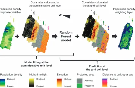
In the RF-based dasymetric population mapping approach developed by Stevens et al.24, a RF algorithm is used to generate gridded population density estimates that are subsequently used to dasymetrically disaggregate population counts from administrative units into grid cells. The same approach was used to produce the WorldPop Americas datasets described in this article. Initially, a population density response variable and a suite of covariates were calculated at the administrative unit level, and then used to fit a RF model for predicting population density at the grid cell level (i.e., to generate the dasymetric weighting layer) with those raster-based covariates having a spatial resolution of 100 m (Fig. 2).
To reduce processing time during the prediction phase, the multi-stage RF estimation technique developed by Stevens et al.24was used. This technique first fits a model using all available covariates and the (log) population density of each administrative unit as the response. Then, a very conservative covariate selection process is performed to reduce the number of covariates that will be used for both the RF model fitting and prediction. To do this the ‘variable’ importance of each covariate27is extracted and each covariate that has a score equal to zero is removed before re-fitting the RF model. This process is then iterated until only covariates with positive scores remain and thus results in the elimination of both redundant covariates and covariates that could negatively impact the prediction.
As in Stevens et al.24, the RF model fitting was performed by generating 500 trees in the forest and setting the number of observations in the terminal nodes equal to one. The fitted RF model was then used to predict population density using only the same reduced set of covariates. For each grid cell, each regression tree in the forest was used to predict a population density value and the average of all predictions was assigned to it as its estimated population density value. If there were not enough observations (i.e., not enough administrative unit population counts) to fit a RF model for a given country, another country located in the same ecozone30was identified and used to fit an appropriate RF model for predicting population density at the grid cell level31.
Subsequently, in both cases, the population density weighting layer was used to dasymetrically disaggregate the administrative unit-based population counts32and produce two gridded population datasets depicting the estimated number of people per grid square and per hectare for the population count year. These datasets were then projected to 2010 (Fig. 3), 2015, and 2020 using UNPD rural and urban growth rates25and also adjusted to match the most recent UNPD estimates at the time of writing25. All tasks described above were entirely performed using the WordPop-RF code (Data Citation 1) described in the Code availability section below and publicly available through the figshare repository. In particular, the code relies on the R statistical environment (version 2.15) and the randomForest package (version 4.6–7) for fitting the RF model at the administrative unit level and predict at the grid cell level, and on the Python programming language (version 2.6; www.python.org) and ArcGIS 10.1 arcpy package for performing the Geographic Information System (GIS)-specific spatial operations required for
Extract population counts from the most recent official population census, estimate, or projection
Match the extracted population counts to their
corresponding administrative units
Calculate population density at the administrative unit level
Process a number of global default datasets
highly correlated with population density into a
set of default raster covariates Supplement and/or replace
default covariates with additional and/or better country-specific covariates Calculate covariate values
at the administrative unit level
Fit a Random Forests model using population density and covariates both calculated at the administrative unit level
Predict population density at the grid cell level using the fitted Random Forests model and the raster
covariates
Use the predicted population density to
dasymetrically disaggregate population counts from administrative
units into grid cells
Figure 1. Schematic overview of the Random Forest (RF)-based dasymetric mapping approach used to
produce the WorldPop Americas datasets (modified from Stevens et al.24). The preparation of the response
variable and covariates is described in the yellow and orange panels, respectively, the RF modelling steps are outlined in in the green panels, and the disaggregation of the input population counts from administrative units into grid cells is described in the blue panel.
dasymetrically disaggregating the population data, projecting them to 2010, 2015 and 2020, and adjusting them to match UNPD estimates (refer to the Supplementary File 1 for a technical description of how the GIS-specific spatial operations are implemented).
Data collection
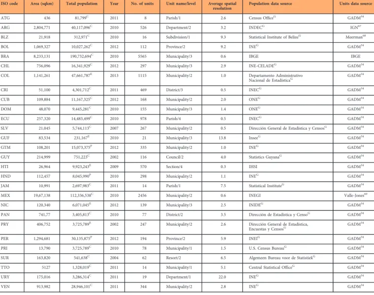
For each country listed in Table 1, population counts were extracted from the most detailed and recent official population count data and matched to their corresponding administrative units in a GIS environment. Both population counts and the corresponding administrative units were either publicly available (e.g., from GeoHive33and GADM34, respectively) or contributed by National Statistical Offices such as the Instituto Brasileiro de Geografia e Estatística (IBGE). Table 1 also provides summary information about the input population count data and administrative unit datasets used to produce the WorldPop Americas datasets.
It is well known that human population density is highly correlated with environmental and physical factors35that can plausibly impact the spatial distribution of population and/or be related to it. These may include continuous variables such as intensity of night-time lights36, energy productivity of plants37, topographic elevation and slope38,39, and climatic factors40, as well as categorical variables such as land-cover type41and presence/absence of roads42, waterways and waterbodies43, human settlements and
ISO code Area (sqkm) Total population Year No. of units Unit name/level Average spatial
resolution Population data source Units data source ATG 436 81,799C 2011 8 Parish/1 2.6 Census OfficeG GADM34
ARG 2,804,771 40,117,096C 2010 526 Department/2 3.2 INDECG IGN67
BLZ 21,918 312,971C 2010 16 Subdivision/1 9.3 Statistical Institute of BelizeG Meerman68
BOL 1,069,327 10,027,262C 2012 112 Province/2 9.2 INEG GADM34
BRA 8,233,131 190,732,694C 2010 5565 Municipality/3 0.6 IBGE IBGE
CHL 756,096 16,341,929C 2012 297 Municipality/3 2.9 INE-CELADEG GADM34
COL 1,141,261 47,661,787E 2013 1115 Municipality/2 1.0 Departamento Administrativo
Nacional de EstadísticaG GADM 34
CRI 51,100 4,301,712C 2011 469 District/3 0.5 INECG GADM34
CUB 109,884 11,167,325C 2012 168 Municipality/2 2.0 ONEG GADM34
DOM 48,070 9,445,281C 2010 155 Municipality/3 1.4 ONEG GADM34
ECU 257,320 14,483,499C 2010 978 Parish/4 0.5 INECG GADM34
SLV 21,045 5,744,113C 2007 267 Municipality/2 0.5 Dirección General de Estadística y CensosG GADM34
GUF 83,534 231,167E 2010 21 Municipality/3 13.8 InseeG GADM34
GTM 108,201 15,073,375P 2012 335 Municipality/2 1.0 INEG GADM34
GUY 214,999 751,223C 2002 116 Council/2 4.0 Statistics GuyanaG GADM34
HTI 26,964 9,923,243E 2009 570 Section/4 0.3 IHSI GADM34
HND 112,457 8,045,990P 2010 298 Municipality/2 1.1 INEG GADM34
JAM 10,991 2,697,983C 2011 14 Parish/1 7.5 Statistical InstituteG GADM34
MEX 19,67,138 112,336,538C 2010 2456 Municipality/2 0.6 INEGI Valle-Jones69
NIC 120,340 6,071,045E 2012 139 Municipality/3 2.5 INIDEG GADM34
PAN 741,77 3,405,813C 2010 77 District/2 3.5 Dirección de Estadística y CensoG GADM34
PRY 406,752 3,725,789E 2002 247 Municipality/2 2.6 Dirección General de Estadística,
Encuestas y CensosG GADM 34
PER 1,294,681 30,135,875P 2012 194 Province/2 5.9 INEIG GADM34
PRI 13,790 3,725,789C 2010 78 Municipality/1 1.5 U.S. Census BureauG GADM34
SUR 163,820 541,638C 2004 62 Resort/2 6.5 Algemeen Bureau voor de StatistiekG GADM34
TTO 5127 1,328,019C 2011 14 Municipality/1 5.1 Central Statistical OfficeG GADM34
URY 175,016 3,286,314C 2011 19 Department/1 22.0 INEG GADM34
VEN 913,982 28,946,101C 2011 344 Municipality/2 2.8 INEG GADM34 Table 1. Summary information about population count data and administrative unit datasets used to produce the WorldPop Americas datasets. For each country (identified by its ISO country code in the 1st column), the Average Spatial Resolution was calculated as the square root of its surface area divided by the number of administrative units and represents the effective resolution of the latter (i.e., the cell size of administrative units
if all units were square of equal size)14. Superscripts ‘C’, ‘E’, and ‘P’, in the 2nd column, indicate whether the
population counts were obtained from either official census, estimates, or projections, respectively. Superscript
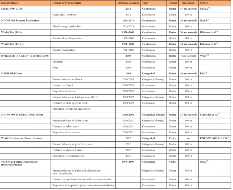
urban areas44, and protected areas45. Thus, twelve global raster and vector datasets (described below) were identified, collected, assembled, and processed into a set of default covariates (Table 2) used for model fitting and prediction.
The spatial variation of factors related to population distribution, such as night-light intensity and plant energy productivity, was measured using the NOAA Suomi National Polar-orbiting Partnership Visible Infrared Imaging Radiometer Suite (VIIRS)46,47and the NASA TERRA/Moderate Resolution Imaging Spectroradiometer (MODIS) Net Primary Productivity (NPP)48,49raster dataset, respectively. The spatial variation of climatic factors affecting population distribution was considered by including the WorldClim Annual Mean Temperature (BIO1) and Annual Precipitation (BIO12) raster datasets50,51. The World Wildlife Fund (WWF) HydroSheds raster dataset52,53, based on the NASA’s Shuttle Radar Topography Mission (SRTM) Digital Elevation Model54, was used to represent the spatial variation of elevation and slope. The European Space Agency (ESA) ENVISAT/MERIS-based GlobCover raster dataset55,56, and the MODIS 500-m map of global urban extent57,58were used to identify different land-cover types and distinguish between urban and rural areas. Finally, the World Database on Protected Areas (WDPA)59was used to obtain vector polygons representing protected areas, while the National
Default dataset Default derived covariate Temporal coverage Type Format Resolution Source Suomi NPP-VIIRS 2012 Continuous Raster 15 arc seconds NOAA46
Night-lights’ intensity 2012 Continuous Raster 100 m
MODIS Net Primary Production 2014/2015 Continuous Raster 30 arc seconds NASA48
Plants’ energy productivity 2014/2015 Continuous Raster 100 m
WorldClim (BIO1) 1950–2000 Continuous Raster 30 arc seconds Hijmans et al.50
Annual Mean Temperature 1950–2000 Continuous Raster 100 m
WorldClim (BIO12) 1950–2000 Continuous Raster 30 arc seconds Hijmans et al.50.
Annual Precipitation 1950–2000 Continuous Raster 100 m
HydroSheds (3 s GRID: Void-filled DEM) 2000 Continuous Raster 3 arc seconds WWF52
Elevation 2000 Continuous Raster 100 m Slope 2000 Continuous Raster 100 m MERIS GlobCover 2009 Categorical Raster 10 arc seconds ESA55
Presence/absence of class # 2000/2009 Categorical (binary) Raster 100 m Distance to class # 2000/2009 Continuous Raster 100 m Proportion of class # 2000/2009 Continuous Raster 100 m Presence/absence of built-up areas (BLT) 2000/2009 Categorical (binary) Raster 100 m Distance to built-up areas (BLT) 2000/2009 Continuous Raster 100 m Proportion of built-up area (BLT)
MODIS 500 m Global Urban Extent 2000/2001 Categorical (binary) Raster 15 arc seconds Schneider et al.57
Presence/absence of urban areas 2000/2001 Categorical (binary) Raster 100 m Distance to urban areas 2000/2001 Continuous Raster 100 m Proportion of urban area 2000/2001 Continuous Raster 100 m
World Database on Protected Areas 2012 Categorical Vector — UNEP-WCMC & IUCN59
Presence/absence of protected areas 2012 Categorical (binary) Raster 100 m Distance to protected areas 2012 Continuous Raster 100 m Proportion of protected area 2012 Continuous Raster 100 m VMAP0 populated places/roads/
rivers/waterbodies 1979–1999 Categorical Vector — NGA
60
Presence/absence of populated places/roads/
rivers/waterbodies Categorical (binary) Raster 100 m Distance to populated places/roads/rivers/waterbodies Continuous Raster 100 m Proportion of populated places/roads/rivers/waterbodies Continuous Raster 100 m
Table 2. Summary information on the twelve default datasets and the derived default covariates used for input to the RF method. Continuous raster datasets were resampled for being used as covariates, while both categorical raster and rasterized vector data sets were firstly resampled and then processed into ‘presence/ absence’, ‘distance to’, and ‘proportion of’ raster covariates. ‘Class #’, in the 2nd column, refers to the WorlPop Americas classes described in Supplementary Table 1. Refer to the Data preparation sub-section below for a more detailed description of how default covariates were processed.
Geospatial-Intelligence Agency (NGA) Vector Map Level 0 (VMAP0) dataset60was used to obtain features representing populated places, roads, rivers, and waterbodies.
Where available, additional country-specific datasets were used to integrate and/or replace the default datasets outlined above and the corresponding default covariates in the analysis. For example, for most of the countries, the Landsat TM-based EarthSat GeoCover-LC raster dataset61,62was combined with the GlobCover raster dataset to refine the extent of urban areas and identify rural settlements. Similarly, OpenStreetMap (OSM) vector datasets63were regularly used to integrate the VMAP0 settlement dataset and account for land-use types, building sites, and locations of points of interest that may be strongly correlated with population presence (e.g., health clinics, schools, and police stations). Furthermore, OSM road and river data were often deemed to be more complete than the corresponding VMAP0 data and, thus, were used to increase the precision and accuracy of the gridded population outputs64.
For each country, all assembled vector and raster datasets, including the country specific ones, are described in the metadata file accompanying the corresponding gridded population datasets and viewable in any web-browser (refer to the Data Record section below for a more detailed description of the metadata file content).
Data preparation
For each country, the vector dataset representing its administrative units, used to match to population counts, was projected using the most appropriate country-specific projected coordinate system that minimized linear and areal distortion. It was then buffered by 10 km, and rasterized at a spatial resolution of 100 m. This was done in order to (i) generate a dataset representing the population density response variable, (ii) obtain a raster dataset, representing the study area, for co-registering all raster covariates, and (iii) produce a number of raster ‘distance to’ covariates that were unaffected by edge effects due to the fact that the study area is artificially bounded while spatial processes are not65. The population density response variable was obtained through dividing population counts by the area of the corresponding administrative units, and log-transforming the results to normalize the response variable distribution.
Covariates for input to the RF method were derived as follows. First, a continuous raster dataset representing the spatial variation of topographic slope was derived from the USGS HydroSheds dataset (Table 2). Then, all raster datasets representing continuous variables, including the latter, were projected, resampled to 100 m resolution, co-registered and matched to the rasterized buffered study area. For all covariates, ‘NoData’ grid cells overlapping the rasterized buffered study area were filled with the values of the nearest neighbours (using the Nibble tool available in ArcGIS 10.1). All vector and raster datasets representing categorical variables were projected, rasterized to or resampled to 100 m resolution, co-registered, matched to the rasterized buffered study area, and converted into a number of binary raster covariates, representing presence/absence of a given feature, that were subsequently used to produce continuous ‘distance to’ and ‘proportion of’ raster covariates (Table 2); with the latter representing, within a 500 m buffer from each grid cell, the proportion of grid cells where the given feature is present. A special case of a categorical raster dataset is the land-cover data. Indeed, in this case land-cover classes must be aggregated (if needed) and recoded to match the ten WorlPop Americas classes derived
Random Forest model Population density response variable Covariates calculated at
the administrative unit level Covariates calculatedthe at grid cell level
Population density weighting layer
Model fitting at the
administrative unit level Prediction at the grid cell level
Population density Night-time light Elevation Protected area Distance to built-up areas
Highest Brightest Highest Absence Farthest Lowest Darkest Lowest Presence Closest
Figure 2. Schematic overview of the procedure used to generate population density weighting layers. For illustrative purpose, only 4 out of the 74 covariates considered for Puerto Rico are shown here (the uninhabited Puerto Rican islands of Mona, Monito, and Desecheo are not shown).
from the GlobCover dataset (i.e., from class 11 to 230 in the 4th column of Supplementary Table 1). By default, the recoded GlobCover dataset was ‘Nibbled’, to fill in any missing grid cell, and then mosaicked with the MODIS 500 m Global Urban Extent dataset to delineate the extent of urban and non-urban built-up areas (i.e., class 190 and 240 respectively in Supplementary Table 1). When using the GeoCover-LC dataset, it was first recoded and mosaicked with the GlobCover dataset, to fill missing grid cell, and with the MODIS 500 m Global Urban Extent dataset. Similarly to the other raster datasets representing categorical variables, the processed land-cover raster dataset obtained as described above was projected, resampled to 100 m resolution, co-registered, matched to the rasterized buffered study area, and converted into twelve binary raster covariates including the combined built-up areas class (BLT) obtained by combining classes 190 and 240. Binary raster covariates were subsequently used to produce continuous ‘distance to’ and ‘proportion of’ raster covariates (Table 2). Finally, average and modal values for continuous and binary covariates, respectively, were calculated for each administrative unit and used for fitting the RF model.
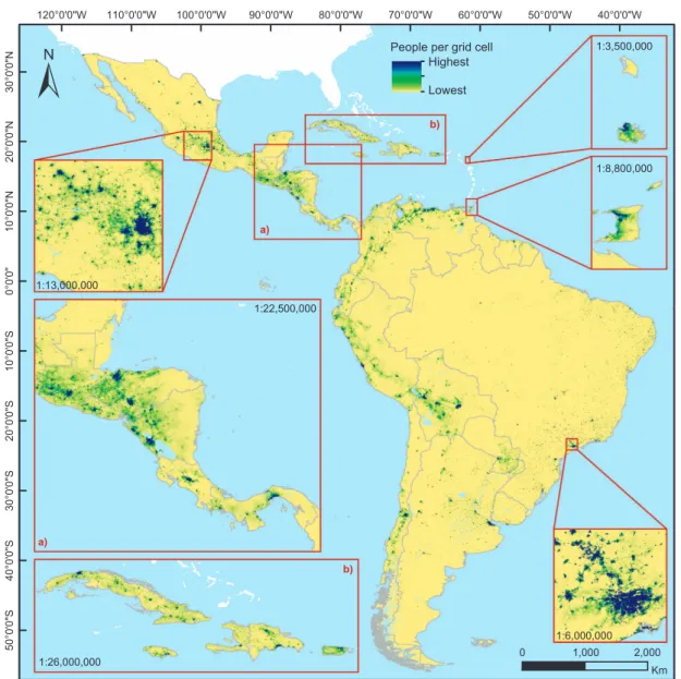
a) b) 30°0'0"N 20°0'0"N 10°0'0"N 0°0'0" 10°0'0"S 20°0'0"S 30°0'0"S 40°0'0"S 50°0'0"S 40°0'0"W 50°0'0"W 60°0'0"W 70°0'0"W 80°0'0"W 90°0'0"W 100°0'0"W 110°0'0"W 120°0'0"W
People per grid cell Highest Lowest 1:8,800,000 1:3,500,000 b) a) 1:13,000,000 1:22,500,000 1:26,000,000 0 1,000 2,000Km 1:6,000,000
Figure 3. Estimated people per grid cell for Latin America and the Caribbean in 2010 (excluding Guadalupe, Martinique, Bahamas, Barbados, Saint Lucia, Curaçao, Aruba, Saint Vincent and The Grenadines, US and British Virgin Islands, Grenada, Dominica, Cayman Islands, Saint Kitts and Nevis, Sint Maarten, Turks and Caicos Islands, Saint Martin, Caribbean Netherlands, Anguilla, Saint Barthélemy, and Montserrat). The grid cell resolution is 3 arc seconds (approximately 100 m at the equator) and coordinates refer to GCS WGS 1984. For illustrative purpose, the color ranges used are country-specific.
The preparation of the population density response variable and raster covariates was entirely performed using the WordPop-RF code (Data Citation 1) described in the Code availability section below and publicly available through the figshare repository. In particular, the code relies on the Python programming language (version 2.6; www.python.org) and ArcGIS 10.1 arcpy package for performing the GIS-specific spatial operations required for preparing both the response variable and raster covariates (refer to the Supplementary File 1 for a technical description of how the GIS-specific spatial operations are implemented). For each country, all derived covariates are listed in the metadata file accompanying the corresponding gridded population datasets (refer to the Data Record section below for a more detailed description of the metadata file contents).
Code availability
The WordPop-RF code (Data Citation 1), used to produce the WorldPop Americas datasets, as well as the metadata and the KML files associated with them (refer to the Data Records section for a description of the latter), is publicly available through the figshare repository. The code consists of two Python (version 2.6; www.python.org) and four R (version 2.15.3) programming language scripts that must be run sequentially in the following order: 1) 01.0—Configuration.py.R; 2) Metadata.R; 3) 01.1—Data Preparation, R.r; 4) 01.2—Data Preparation, Python.py; 5) 01.3—More Complex Random Forest Regression, Full Covariate Set and Data Preparation.r; 6) 01.4—Process Density Weights to Population Maps.py; 7) 01.5—Generate KML.r; 8) 01.6—Generate Metadata Report.r. Each script is also internally documented in order to both explaining its purpose (including a detailed description of the GIS-specific spatial operations that it performs) and, when required, guiding the user through its customization.
Data Records
The high-resolution WorldPop Americas datasets described in this article referring to the 28 countries listed in Table 1, are publicly and freely available both through the WorldPop Dataverse Repository (Data Citation 2) and the WorldPop project website (http://www.worldpop.org.uk/data/). However, while the WorldPop Americas datasets stored in the Dataverse Repository represent a static version of the datasets produced at the time of writing and will be preserved stably in their published form, the datasets stored in the project website (Supplementary Table 2) will be expanded by including additional countries located in the region and updated as better and more recent official population count data and covariates become available.
Both through the Dataverse Repository and the project website, the WorldPop Americas can be download as 7-Zip archives (7-Zip.org) containing the population distribution datasets of the country it is associated with for the population count year, as well as for 2010, 2015, and 2020, and a RF model metadata report (Table 3).
Additionally, from the Data Availability page available on the WorldPop project website (http://www. worldpop.org.uk/data/data_sources/) it is also possible to browse the 7-Zip archives described above, download individual GeoTIFF datasets from them, and view the HTML files containing the RF model
Name Description (resolution) Format ISO_ppp_v2b_YEAR.tif Estimated people per grid cell for the year the official population count data refer to (3 arc seconds) GeoTIFF ISO_ppp_v2b_2010.tif Projected estimated people per grid cell for 2010 (3 arc seconds) GeoTIFF ISO_ppp_v2b_2010_UNadj.tif Projected estimated people per grid cell for 2010 adjusted to match UNPD estimates (3 arc seconds) GeoTIFF ISO_ppp_v2b_2015.tif Projected estimated people per grid cell for 2015 (3 arc seconds) GeoTIFF ISO_ppp_v2b_2015_UNadj.tif Projected estimated people per grid cell for 2015 adjusted to match UNPD estimates (3 arc seconds) GeoTIFF ISO_ppp_v2b_2020.tif Projected estimated people per grid cell for 2020 (3 arc seconds) GeoTIFF ISO_ppp_v2b_2020_UNadj.tif Projected estimated people per grid cell for 2020 adjusted to match UNPD estimates (3 arc seconds) GeoTIFF ISO_pph_v2b_YEAR.tif Estimated people per hectare for the year the official population count data refer to (3 arc seconds) GeoTIFF ISO_pph_v2b_2010.tif Projected estimated people per hectare for 2010 GeoTIFF ISO_pph_v2b_2010_UNadj.tif Projected estimated people per hectare for 2010 adjusted to match UNPD estimates (3 arc seconds) GeoTIFF ISO_pph_v2b_2015.tif Projected estimated people per hectare for 2015 GeoTIFF ISO_pph_v2b_2015_UNadj.tif Projected estimated people per hectare for 2015 adjusted to match UNPD estimates (3 arc seconds) GeoTIFF ISO_pph_v2b_2020.tif Projected estimated people per hectare for 2020 (3 arc seconds) GeoTIFF ISO_pph_v2b_2020_UNadj.tif Projected estimated people per hectare for 2020 adjusted to match UNPD estimates (3 arc seconds) GeoTIFF
ISO_ppp_v2b_YEAR.kmz Estimated people per grid cell for the year the official census/population counts refer to Keyhole Markup Language (Zipped) ISO_metadata.html Metadata report for the Random Forest model HyperText Markup Language
Table 3. Name (ISO and YEAR represent the ISO country code and the population count year, respectively), description, and format of all files contained in each 7-Zip archive associated with the 28 countries listed in Table 1.
metadata reports. For each country, the metadata report illustrates the datasets and the related derived covariates used as input in the RF model, the population density response variable, the gridded population density dataset used to dasymetrically disaggregate the population from administrative unit to grid cell level, and basic information about the RF model that includes (i) the country on which it is
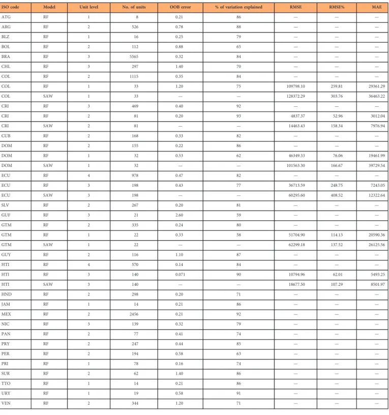
ISO code Model Unit level No. of units OOB error % of variation explained RMSE RMSE% MAE
ATG RF 1 8 0.21 86 — — — ARG RF 2 526 0.78 88 — — — BLZ RF 1 16 0.25 79 — — — BOL RF 2 112 0.88 65 — — — BRA RF 3 5565 0.32 84 — — — CHL RF 3 297 1.40 70 — — — COL RF 2 1115 0.35 84 — — — COL RF 1 33 1.20 75 109798.10 259.81 29361.29 COL SAW 1 33 — — 128372.29 303.76 36463.22 CRI RF 3 469 0.40 92 — — — CRI RF 2 81 0.20 93 4837.37 52.96 3012.04 CRI SAW 2 81 — — 14463.43 158.34 7976.94 CUB RF 2 168 0.33 82 — — — DOM RF 2 155 0.22 86 — — — DOM RF 1 32 0.53 62 46349.33 76.06 19461.99 DOM SAW 1 32 — — 101563.30 166.67 39729.54 ECU RF 4 978 0.47 82 — — — ECU RF 3 198 0.43 77 36713.59 248.75 7243.05 ECU SAW 3 198 — — 60295.60 408.52 12322.64 SLV RF 2 267 0.20 81 — — — GUF RF 3 21 2.60 59 — — — GTM RF 2 335 0.24 80 — — — GTM RF 1 22 0.33 58 51704.90 114.13 20590.36 GTM SAW 1 22 — — 62299.18 137.52 26125.56 GUY RF 2 116 1.10 87 — — — HTI RF 4 570 0.14 84 — — — HTI RF 3 140 0.071 90 10794.96 62.01 5493.25 HTI SAW 3 140 — — 18677.50 107.29 8501.97 HND RF 2 298 0.20 71 — — — JAM RF 1 14 0.21 86 — — — MEX RF 2 2456 0.21 92 — — — NIC RF 3 139 0.32 79 — — — PAN RF 2 77 0.41 74 — — — PRY RF 2 247 0.44 85 — — — PER RF 2 194 0.58 63 — — — PRI RF 1 78 0.16 74 — — — SUR RF 2 62 1.40 86 — — — TTO RF 1 14 0.21 86 — — — URY RF 1 19 0.58 91 — — — VEN RF 2 344 1.20 71 — — —
Table 4. Prediction accuracy of the RF model used to generate the dasymetric weighting layers and accuracy assessment of the RF-based dasymetric mapping approach compared to the simple areal-weighting (SAW) mapping approach. The OOB error and the percentage of variance explained are provided for all 28 countries while the RMSE, the %RMSE, and the MAE values are provided for six countries. ‘RF’ and ‘SAW’, in the 2nd column, indicate that, for that specific country, the population counts at the administrative unit level were disaggregated using the RF-based dasymetric mapping approach and the simple areal-weighting approach, respectively.
based, (ii) its prediction error, (iii) the relative importance of each covariate, (iv) the prediction intervals using the OOB data (refer to the Methods section for additional information about the latter features).
Technical Validation
Root mean square error (RMSE) and mean absolute error (MAE)
Six countries, located in different parts of the Latin American and the Caribbean region were selected to assess the increased accuracy of the RF-based dasymetric mapping approach with respect to a simple areal-weighting (SAW) approach66 (Table 4). For each selected country, population counts were aggregated within the next coarser administrative level boundary than the finest for which they were available (e.g., if admin level 4 population count data were available, these were aggregated to admin level 3). The coarser, aggregated population counts were then used to produce gridded population count datasets, with a resolution of 100 m, using both the SAW and the RF approach outlined here. Finally, the two different population estimates produced using these approaches within each of the finest administrative unit were calculated, and compared with observed population figure referring to the same higher resolution unit.
Results, summarized in Table 4, show how both the RMSE, the %RMSE (RMSE expressed as a percentage of the average population of the finest administrative unit level), and the MAE values (5th, 6th, and 7th column of Table 4, respectively) calculated using the RF-based outputs are consistently lower than the corresponding values calculated for the SAW outputs. These statistics can be used to compare the accuracy of the two approaches when downscaling the estimates.
Out-of-bag (OOB) error estimation
The OOB error estimate (3rd column of Table 4), as already briefly described in the Methods section, is internally calculated during the RF model fitting and can be considered a robust and unbiased measurement of the prediction accuracy of the model itself27.
Nevertheless, it is important to note that since the RF model is fitted at the administrative unit level and then is used to predict at the grid cell level, the OOB error estimate should not be interpreted as the prediction error at the grid cell level. Similarly, it does not represent the prediction error that could be expected to be observed at the administrative unit level by summing all final grid cell values within each administrative unit and comparing it to the observed population count referring to the same administrative unit. However, referring to the six countries mentioned in the previous section, by comparing the OOB error estimates calculated at the aggregate lower administrative unit level than the highest available (3rd column of Table 4) with the corresponding RMSE and MAE values (5th and 7th column of Table 3, respectively), it is reasonable to expect that higher accuracy of predicted values at the administrative unit level results in a higher accuracy of the final gridded population distribution datasets24.
Usage Notes
The WorldPop Americas datasets can be used both to support applications for planning interventions, measuring progress, and to predict response variables intrinsically dependent on the population distribution. However, considering that they represent modelling outputs generated using ancillary covariate datasets in the disaggregation process, to avoid circularity, they should not be used to make predictions or explore relationships about any of these ancillary datasets14. Thus, before using WorldPop Americas datasets in correlation analyses against factors which are included in the process of their construction (e.g., correlating population distribution with land-cover), ideally the population modelling process should be re-run using the WordPop-RF code (Data Citation 1) with the covariate of interest being removed to avoid issues relating to endogeneity.
References
1. United Nations, Department of Economic and Social Affairs, Population Division (UNPD). World Urbanization Prospects: The 2014 Revision, Highlights. (United Nations, 2014).
2. Pan American Health Organization (PAHO). Health in the Americas, 2012 Edition: Regional Volume, http://www2.paho.org/ saludenlasamericas/dmdocuments/hia-2012-chapter-4.pdf (2012).
3. World Health Organisation (WHO). The Global Burden of Disease: 2004 Update. (World Health Organisation, 2008). 4. World Health Organisation (WHO). The World Health Report 2013: Research for Universal Health Coverage. (World Health
Organisation, 2013).
5. International Federation of Red Cross and Red Crescent Societies (IFRC). World Disaster Report 2014: Focus on Culture and Risk. (Imprimerie Chirat, 2014).
6. Intergovernmental Panel on Climate Change (IPCC). Climate Change 2014: Synthesis Report. Contribution of Working Groups I, II and III to the Fifth Assessment Report of the Intergovernmental Panel on Climate Change. (IPCC, 2014).
7. Grau, H. R. & Aide, M. Globalization and land-use transitions in Latin America. Ecology and Society 13, 16 (2008). 8. United Nations Human Settlements Programme (UN-Habitat). State of the world’s cities 2012/2013: Prosperity of cities.
(Routledge, 2012).
9. McDonald, R. I. et al. Urban growth, climate change, and freshwater availability. Proc. Natl. Acad. Sci 108, 6312–6317 (2011). 10. Brown, M. L., Donovan, T. M., Schwenk, W. S. & Theobald, D. M. Predicting impacts of future human population growth and
development on occupancy rates of forest-dependent birds. Biol. Conser 170, 311–320 (2014).
11. McGranahan, G., Balk, D. & Anderson, B. The rising tide: assessing the risks of climate change and human settlements in low elevation coastal zones. Environ. Urban. 19, 17–37 (2007).
12. Tatem, A. J., Campiz, N., Gething, P. W., Snow, R. W. & Linard, C. The effects of spatial population dataset choice on estimates of population at risk of disease. Population Health Metrics 9, 4 (2011).
13. Taramelli, A., Melelli, L., Pasqui, M. & Sorichetta, A. Modelling risk hurricane elements in potentially affected areas by a GIS system. Geomatics, Natural Hazards and Risk 1, 349–373 (2010).
14. Balk, D. L., Deichmann, U., Yetman, G., Pozzi, F., Hay, S. I. & Nelson, A. Determining Global Population Distribution: Methods, Applications and Data. Adv. Parasit 62, 119–156 (2006).
15. Tobler, W., Deichmann, U., Gottsegen, J. & Maloy, K. World population in a grid of spherical quadrilaterals. International Journal of Population Geography 3, 203–225 (1997).
16. Deichmann, U., Balk, D. & Yetman, G. Transforming Population Data for Interdisciplinary Usages: From Census to Grid http://sedac.ciesin.org/gpw-v2/GPWdocumentation.pdf (Center for International Earth Science Information Network (CIESIN), Columbia University, 2001).
17. Balk, D. & Yetman, G. The Global Distribution of Population: Evaluating the gains in resolution refinement
http://sedac.ciesin.columbia.edu/downloads/docs/gpw-v3/gpw3_documentation_final.pdf (Center for International Earth Science Information Network (CIESIN), Columbia University, 2004).
18. Doxsey-Whitfield, E. et al. Taking Advantage of the Improved Availability of Census Data: A First Look at the Gridded Population of the World, Version 4. Papers in Applied Geography 1, 226–234 (2015).
19. Balk, D., Pozzi, F., Yetman, G., Deichmann, U. & Nelson, A. The distribution of people and the dimension of place: methodologies to improve the global estimation of urban extents. In Proc. of 2005 Urban Remote Sensing Conference ftp://ftp.ecn.purdue.edu/jshan/proceedings/URBAN_URS05/balk-etal.pdf (2005).
20. Dobson, J. E., Bright, E. A., Coleman, P. R., Durfee, R. C. & Worley, B. A. LandScan: a global population database for estimating populations at risk. Photogramm. Eng. Rem. S 66, 849–857 (2000).
21. Centro Internacional de Agricultura Tropical (CIAT)United Nations Environment Program (UNEP) Center for International Earth Science Information Network (CIESIN) Columbia Universitythe World Bank. Latin America and the Caribbean Population Database http://gisweb.ciat.cgiar.org/population/download/report.pdf (CIAT, 2000).
22. Linard, C., Gilbert, M., Snow, R. W., Noor, A. M. & Tatem, A. J. Population Distribution, Settlement Patterns and Accessibility across Africa in 2010. PLoS ONE 7, e31743 (2012).
23. Gaughan, A. E., Stevens, F. R., Linard, C., Jia, P. & Tatem, A. J. High Resolution Population Distribution Maps for Southeast Asia in 2010 and 2015. PLoS ONE 8, e55882 (2013).
24. Stevens, F. R., Gaughan, A. E., Linard, C. & Tatem, A. J. Disaggregating Census Data for Population Mapping Using Random Forests with Remotely-Sensed and Ancillary Data. PLoS ONE 10, e0107042 (2015).
25. United NationsDepartment of Economic and Social AffairsPopulation Division (UNPD). World Urbanization Prospects: The 2014 Revision. CD-ROM Editionhttp://esa.un.org/unpd/wup/CD-ROM/ (2014).
26. Breiman, L. Bagging predictors. Mach. Learn. 24, 123–140 (1996). 27. Breiman, L. Random forests. Mach. Learn. 45, 5–32 (2001).
28. Liaw, A. & Wiener, M. Classification and Regression by randomForest. R News 2, 18–22 (2002).
29. Breiman, L. Manual on setting up, using, and understanding random forests v3.1 http://www.stat.berkeley.edu/~breiman/ Using_random_forests_V3.1.pdf (2002).
30. Kottek, M., Grieser, J., Beck, C., Rudolf., B. & Rubel, F. World map of the Koppen-Geiger climate classification updated. Meteorol. Z. 15, 259–263 (2006).
31. Gaughan, A. E., Stevens, F. R., Linard, C., Patel, N. N. & Tatem, A. J. Exploring nationally and regionally defined models for large area population mapping. Int. J. Digit. Earth.doi:10.1080/17538947.2014.965761 (2014).
32. Mennis, J. Generating Surface Models of Population Using Dasymetric Mapping. The Professional Geographer 55, 31–42 (2003). 33. GEOHIVE. Global Population Statistics http://www.geohive.com/cntry/ (2014).
34. GADM. Database of Global Administrative Areas http://www.gadm.org/ (2012).
35. Nagle, N. N., Buttenfield, B. P., Leyk, S. & Spielman, S. Dasymetric Modeling and Uncertainty. Ann. Assoc. Am. Geogr 104, 80–95 (2014).
36. Briggs, D. J., Gulliver, J., Fecht, D. & Vienneau, D. M. Dasymetric modelling of small-area population distribution using land cover and light emissions data. Remote Sens. Environ. 108, 451–466 (2007).
37. Luck, J. W. The relationships between net primary productivity, human population density and species conservation. J. Biogeogr. 34, 201–212 (2007).
38. Cohen, J. E. & Small, C. Hypsographic demography: The distribution of human population by altitude. Proc. Natl. Acad. Sci 95, 14009–14014 (1998).
39. Schumacher, J. V., Redmond, R. L., Hart, M. M. & Jensen, M. E. Mapping patterns of human use and potential resource conflicts on public lands. Environ. Monit. Assess. 64, 127–137 (2000).
40. Small, C. & Cohen, J. E. Continental physiography, climate, and the global distribution of human population. Curr. Anthropol. 45, 269–277 (2004).
41. Linard, C., Gilbert, M. & Tatem, A. J. Assessing the use of global land cover data for guiding large area population distribution modelling. GeoJ 76, 525–538 (2011).
42. Reibel, M. & Bufalino, M. E. Street-weighted interpolation techniques for demographic count estimation in incompatible zone systems. Environ. Plann. A 27, 127–139 (2005).
43. Kummu, M., de Moel, H., Ward, P. J. & Varis, O. How Close Do We Live to Water? A Global Analysis of Population Distance to Freshwater Bodies. PLoS ONE 6, e20578 (2011).
44. Tatem, A. J., Noor, A. M., von Hagen, C., Di Gregorio, A. & Hay, S. I. High Resolution Population Maps for Low Income Nations: Combining Land Cover and Census in East Africa. PLoS ONE 2, e1298 (2007).
45. Luck, G. W. A review of the relationships between human population density and biodiversity. Biol. Rev. 82, 607–645 (2007). 46. National Oceanic and Atmospheric Administration (NOAA). Visible Infrared Imaging Radiometer Suite (VIIRS) Nighttime
Lights-2012 (Two months composite) http://ngdc.noaa.gov/eog/viirs/download_viirs_ntl.html (2013).
47. Elvidge, C. D., Baugh, K. E., Zhizhi, M. & Hsu, F.-C. Why VIIRS data are superior to DMSP for mapping nighttime lights. Proc. Asia Pac. Adv. Netw 35, 62–19 (2013).
48. National Aeronautics and Space Administration (NASA). Terra/MODIS Net Primary Production Yearly L4 Global 1 km MOD17A3 https://lpdaac.usgs.gov/dataset_discovery/modis/modis_products_table/mod17a3 (2015).
49. Turner, D. P. et al. Evaluation of MODIS NPP and GPP products across multiple biomes. Remote Sens. Environ. 102, 282–292 (2006).
50. Hijmans, R. J., Cameron, S. E., Parra, J. L., Jones, P. G., Jarvis, A. & Richardson, K. WorldClim Annual Mean Temperature (BIO1) and Annual Precipitation (BIO12) 30 arc-seconds (~1 km) http://www.worldclim.org/current (2005).
51. Hijmans, R. J., Cameron, S. E., Parra, J. L., Jones, P. G. & Jarvis, A. Very high resolution interpolated climate surfaces for global land areas. Internat. J. Climatol. 25, 1965–1978 (2005).
53. Lehner, B., Verdin, K. & Jarvis, A. New Global Hydrography Derived From Spaceborne Elevation Data. Eos Trans. AGU 89, 93–94 (2008).
54. Farr, T. G. et al. The shuttle radar topography mission. Rev. Geophys. 45 doi:10.1029/2005RG000183 (2007).
55. European Space Agency (ESA). GlobCover 2009 (Global Land Cover Map) http://due.esrin.esa.int/page_globcover.php (2010). 56. Bontemps, S., Defourny, P., van Bogaert, E., Kalogirou, V. & Arino, O. GlobCover 2009: Products description and
validation report http://due.esrin.esa.int/files/GLOBCOVER2009_Validation_Report_2.2.pdf (2011).
57. Schneider, A., Friedl, M. A. & Potere, D. Mapping global urban areas using MODIS 500-m data: New methods and datasets based on ‘urban ecoregions’. Remote Sens. Environ. 114, 1733–1746 (2010).
58. Schneider, A., Friedl, M. A. & Potere, D. A new map of global urban extent from MODIS satellite data. Environ. Res. Lett. 4, 044003 (2009).
59. United Nations Environment Programme's World Conservation Monitoring Centre (UNEP-WCMC) & International Union for Conservation of Nature (IUCN). World Database on Protected Areas (WDPA) http://www.protectedplanet.net/ (2012). 60. National Geospatial-Intelligence Agency (NGA). VMAP0
http://geoengine.nga.mil/geospatial/SW_TOOLS/NIMAMUSE/webin-ter/rast_roam.html (2005).
61. MDA Federal Inc. EarthSat GeoCover-LC Year 2000 http://www.mdafederal.com/geocover (2005).
62. Cunningham, D., Melican, J. E., Wemmelmann, E. & Jones, T. B. GeoCover LC-A moderate resolution global land cover database. In Proc. of 2002 Esri International User Conference http://proceedings.esri.com/library/userconf/proc02/pap0811/p0811.htm (2002).
63. OpenStreetMap contributors. OpenStreetMap http://www.openstreetmap.org/ (2014).
64. Linard, C. et al. Use of active and passive VGI data for population distribution modelling: experience from the WorldPop project. In Proc. of the Eighth International Conference on Geographic Information Science https://web.ornl.gov/registration_resumes/ CFP_VGI%20Workshop_Linard.pdf (2014).
65. Fotheringham, A. S. & Rogerson, P. A. GIS and spatial analytical problems. Int. J. Geogr. Inf. Syst 7, 3–19 (1993). 66. Flowerdew, R. & Green, M. Areal interpolation and types of data. Spatial analysis and GIS (Taylor and Francis Ltd., 1994). 67. Instituto Geográfico Nacional de la República Argentina (IGN). Departamentos http://www.ign.gob.ar/NuestasActividades/sigign
(2013).
68. Meerman, J. Belize Basemap (boundaries, districts) http://www.biodiversity.bz/mapping/warehouse/ (2010).
69. Valle-Jones, D. Shapefiles of Mexico (AGEBs, Manzanas, etc) https://blog.diegovalle.net/2013/06/shapefiles-of-mexico-agebs-manzanas-etc.html (2013).
Data Citations
1. Stevens, F. R. et al. WorldPop-RF, Version 2b.1.1. figshare http://dx.doi.org/10.6084/m9.figshare.1491490 (2015).
2. Sorichetta, A., Hornby, G. M., Stevens, F. R., Gaughan, A. E., Linard, C. & Tatem, A. J. Americas Datasets, V1. Harvard Dataverse http://dx.doi.org/10.7910/DVN/PUGPVR (2015).
Acknowledgements
A.S. is supported by funding from the Bill & Melinda Gates Foundation (OPP1106427, 1032350). A.J.T. is supported by funding from NIH/NIAID (U19AI089674), the Bill & Melinda Gates Foundation (OPP1106427, 1032350), and the RAPIDD program of the Science and Technology Directorate, Department of Homeland Security, and the Fogarty International Center, National Institutes of Health. This work forms part of the WorldPop Project (www.worldpop.org). The funders had no role in study design, data collection and analysis, decision to publish, and preparation of the manuscript.
Author Contributions
A.S. drafted the manuscript. A.S., G.M.H., and F.R.S. undertook data collection, assembly, and analyses, produced the datasets, and performed their technical validation. F.R.S. developed the Random Forests-based dasymetric mapping approach and the multi-stage Random Forests estimation technique used for producing the datasets. G.M.H., F.R.S., A.E.G., and C.L. edited the manuscript. A.E.G. and C.L. aided with data collection. A.J.T. conceived the study, aided with data collection and drafting the manuscript. All authors read and approved the final version of the manuscript.
Additional Information
Supplementary Information accompanies this paper at http://www.nature.com/sdata
Competing financial interests: The Authors declare that they have no competing financial interests that might have influenced the presentation of the WorldPop Americas datasets and the description of the methods used to produce and assess them.
How to cite this article: Sorichetta, A. et al. High-resolution gridded population datasets for Latin America and the Caribbean in 2010, 2015, and 2020. Sci. Data 2:150045 doi: 10.1038/sdata.2015.45 (2015).
This work is licensed under a Creative Commons Attribution 4.0 International License. The images or other third party material in this article are included in the article’s Creative Commons license, unless indicated otherwise in the credit line; if the material is not included under the Creative Commons license, users will need to obtain permission from the license holder to reproduce the material. To view a copy of this license, visit http://creativecommons.org/licenses/by/4.0
Metadata associated with this Data Descriptor is available at http://www.nature.com/sdata/ and is released under the CC0 waiver to maximize reuse.