HAL Id: hal-01218283
https://hal.archives-ouvertes.fr/hal-01218283
Submitted on 20 Oct 2015
HAL is a multi-disciplinary open access
archive for the deposit and dissemination of
sci-entific research documents, whether they are
pub-lished or not. The documents may come from
teaching and research institutions in France or
abroad, or from public or private research centers.
L’archive ouverte pluridisciplinaire HAL, est
destinée au dépôt et à la diffusion de documents
scientifiques de niveau recherche, publiés ou non,
émanant des établissements d’enseignement et de
recherche français ou étrangers, des laboratoires
publics ou privés.
mouse ([i]Rhabdomys[/i] sp.) : inference from its current
distribution in Southern Africa
Christine Meynard, Neville Pillay, Manon Perrigault, Pierre Caminade, Guila
Ganem
To cite this version:
Christine Meynard, Neville Pillay, Manon Perrigault, Pierre Caminade, Guila Ganem. Evidence of
environmental differentiation in the striped mouse ([i]Rhabdomys[/i] sp.) : inference from its current
distribution in Southern Africa. Ecology and Evolution, Wiley Open Access, 2012, 2 (5), pp.1008-1023.
�10.1002/ece3.219�. �hal-01218283�
striped mouse (Rhabdomys sp.): inference from its current
distribution in southern Africa
Christine N. Meynard1, Neville Pillay2, Manon Perrigault3, Pierre Caminade3& Guila Ganem2,3
1INRA, UMR CBGP (INRA/IRD/Cirad/Montpellier SupAgro), Campus international de Baillarguet, CS 30016, F-34988 Montferrier-sur-Lez cedex, France 2School of Animal, Plant and Environmental Sciences, University of the Witwatersrand, Private Bag 3, WITS 2050, South Africa
3Institut des Sciences de l’Evolution, UMR 5554, Universit ´e Montpellier 2, C.C. 065, Montpellier cedex 5 34095, France
Keywords
MAXENT, niche differentiation, OMI, radiation, Rhabdomys, rodents, southern Africa, speciation, species distribution modelling.
Correspondence
Christine N. Meynard, INRA, UMR CBGP (INRA/IRD/Cirad/Montpellier SupAgro), Campus international de Baillarguet, CS 30016, F-34988 Montferrier-sur-Lez cedex, France. Tel: +33-4 30 63 04 29;
Fax: (33) 4 99 62 33 45;
E-mail: Christine.Meynard@supagro.inra.fr This study is part of an international program of scientific collaboration financed by the NRF (South Africa) and the CNRS (France): PICS n◦4841. We have also benefited from financial
and scientific support from the GDRI 191 and the University of the Witwatersrand. Received: 3 February 2012; Accepted: 3 February 2012
Ecology and Evolution 2012; 2(5):
1008–1023
doi: 10.1002/ece3.219
Abstract
The aim of this study was to characterize environmental differentiation of lineages within Rhabdomys and provide hypotheses regarding potential areas of contact between them in the Southern African subregion, including the Republic of South Africa, Lesotho, and Namibia. Records of Rhabdomys taxa across the study region were compiled and georeferenced from the literature, museum records, and field expeditions. Presence records were summarized within a 10× 10 km grid covering the study area. Environmental information regarding climate, topography, land use, and vegetation productivity was gathered at the same resolution. Multivariate statistics were used to characterize the current environmental niche and distribution of the whole genus as well as of three mitochondrial lineages known to occur in southern Africa. Distribution modeling was carried out using MAXENT in order to generate hypotheses regarding current distribution of each taxa and their potential contact zones. Results indicate that the two species within Rhabdomys appear to have differentiated across the precipitation/temperature gradient present in the region from east to west. R. dilectus occupies the wettest areas in eastern southern Africa, while R. pumilio occupies the warmer and drier regions in the west, but also penetrates in the more mesic central part of the region. We provide further evidence of environmental differentiation within two lineages of R. dilectus. Contact zones between lineages appear to occur in areas of strong environmental gradients and topographic complexity, such as the transition zones between major biomes and the escarpment area where a sharp altitudinal gradient separates coastal and plateau areas, but also within more homogeneous areas such as within grassland and savannah biomes. Our results indicate that Rhabdomys may be more specialized than previously thought when considering current knowledge regarding mitochondrial lineages. The genus appears to have differentiated along two major environmental axes in the study region, but results also suggest dispersal limitations and biological interactions having a role in limiting current distribution boundaries. Furthermore, the projection of the potential geographic distribution of the different lineages suggests several contact zones that may be interesting study fields for understanding the interplay between ecological and evolutionary processes during speciation.
Introduction
The factors that determine species distributions have a long standing interest for ecologists (MacArthur 1982; Begon et al. 1996; Gaston 2003; Franklin 2009). Species
distribu-tions at large scales have traditionally been linked to cli-matic tolerances and broad-scale environmental conditions (MacArthur 1982; Guisan and Thuiller 2005). Variables such as mean and maximum temperatures have commonly been linked to physiological constraints that limit animal ranges
at high latitudes or high altitudes (Graham et al. 2010; Rowe et al. 2010; Chen et al. 2011). Other commonly cited envi-ronmental variables include precipitation during the harshest months of the year, for example, the driest periods in desert habitats or the coldest periods in subpolar regions (Franklin 2009; Graham et al. 2010). Vegetation productivity, incorpo-rated either through the use of satellite-derived vegetation indices or through an interaction between temperature and precipitation, has also been used frequently to model ani-mal distributions because it can greatly affect resource avail-ability and cover for mobile species (Buckley 2008; Franklin 2009). Finally, various environmental characteristics derived from altitude have been used to represent topographic hetero-geneity that may be an important limiting factor to disper-sal and persistence in vertebrate populations (Franklin 2009; Rissler and Smith 2010; Rowe et al. 2010). Overall, the use of these multiple large-scale environmental predictors to project potential species distributions has proven highly successful in a variety of contexts (Graham et al. 2004; Guisan and Thuiller 2005; Elith and Leathwick 2009).
However, historic climate fluctuations are also known to influence the current geographical distribution of organisms, potentially leading to disjoint distribution patterns (Cruzan and Templeton 2000), reduced gene flow, and speciation because of diverging stochastic and selective pressures. Ro-dents rely on vegetation for food and cover, so by influ-encing the distribution of vegetation types, climate changes probably have had a major influence on their distribution (Frey 1992; Denys 1999). For example, Russo et al. (2010) explained the current patterns of diversification of the Na-maqua rock mouse (Micaelamys namaquensis), a southern African rodent, through a series of arid periods associated with grassland expansions and savannas contractions during the Miocene and Pliocene (DeMenocal 2004). Drier periods fragmented species ranges into several small refuges, creating the opportunity for reproductive isolation and differentia-tion (Russo et al. 2010). Wetter periods allowed secondary contact between populations, generating the opportunity for either divergent selection or remixing of previously differ-entiated populations (Rundle and Nosil 2005; Rissler and Smith 2010). Similar explanations have been invoked to ex-plain patterns of diversification among a variety of taxonomic groups and biogeographic regions such as the diversification of South American Ctenomys species (Mirol et al. 2010) and of South American birds (Fjeldsa et al. 1999; Herzog et al. 2005; Porzecanski and Cracraft 2005). Importantly, understanding current biogeographic patterns requires both taxonomic and range information to be available for a wide variety of taxa in a given geographic area. For example, the identification of suture zones, that is, areas in which several secondary con-tact zones overlap within a taxonomic group, has provided important evidence that mountain ranges can act as bio-diversity drivers in periods of climate change (Moritz et al.
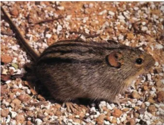
Figure 1. African striped mouse.
2009; Rissler and Smith 2010). However, identifying such ar-eas presupposes the existence of current distribution maps and taxonomic definitions for the taxonomic group under scrutiny.
Many African rodents are believed to have radiated around 3 million years ago, possibly filling newly emerging habi-tats in a period of major environmental changes (Lecompte et al. 2008). Among them, many were traditionally consid-ered as monospecific but were recently shown to display cryp-tic molecular divergence (Rambau et al. 2003; Nicolas 2006; Russo et al. 2010). However, the distribution ranges of these newly described lineages are often poorly known as well as their ecological characteristics and the mechanisms involved in their diversification. The African striped mouse (Fig. 1) belonging to the genus Rhabdomys exemplifies this problem. Rhabdomys belongs to the family Muridae, one of the most diverse rodent families for which southern Africa represents an important centre of endemism (Lecompte et al. 2008). Historically, Rhabdomys was regarded as monospecific, com-prised only of the species R. pumilio (De Graaff 1981). How-ever, recent mitochondrial DNA investigations have indicated the existence of two well-differentiated lineages leading the authors to propose two species names: R. pumilio described in the western (semi arid to arid) part of southern Africa, and R. dilectus described in the eastern part (mesic to hu-mid) (Rambau et al. 2003). These authors also suggested further subdivisions within R. dilectus, with R. d. dilectus in the north and R. d. chakae in the south (Rambau et al. 2003). More recently, preliminary reports from ongoing studies have suggested even more subdivisions within the genus (Castiglia et al. 2011), indicating that the taxonomy of the genus needs revision. Moreover, laboratory crosses showing reduced fer-tility between these proposed species and subspecies (Pillay 2000) as well as evidence of diverging sexual recognition
signals (Pillay et al. 2006) tends to validate these new taxo-nomic subdivisions.
Despite the fact that some differences in social systems and behavioural characteristics have been described within the genus (Schradin and Pillay 2005a; Pillay et al. 2006), envi-ronmental differentiation between the three taxa described above has not been previously formalized. The genus Rhab-domys is still described as a generalist clade because it occupies a variety of habitats, ranging from wet tropical areas to drier semiarid regions (Skinner and Chimimba 2005). However, the description of several lineages within Rhabdomys, and a better knowledge of their distribution create the possibility that the lineages might be specialized to different types of environments, and that the generalist label may therefore be questionable.
The specific aims of this study were to assess whether envi-ronmental differentiation parallels taxonomic diversification within Rhabdomys in southern Africa, to generate hypothe-ses regarding the potential distributions and contact zones between these taxa, and to discuss these results in the context of current climate and biogeography. We would expect the different taxa to differentiate along the major humidity and seasonality gradients present in southern Africa from east to west and from deserts to grasslands to savannas. Further-more, based on dates of divergence provided in Rambau et al. (2003) and paleoclimatic information (DeMenocal 2004), we expect lineages of R. pumilio to have diverged in the arid west-ern part of the southwest-ern African region and R. dilectus in the more humid eastern part of the southern African region. Here, we used multivariate statistics to relate the occurrence of lineages of genetically identified individuals with current environmental conditions. Furthermore, we produced spa-tial hypotheses of potenspa-tial ranges for each lineage by using species distribution modeling in order to identify potential secondary contact zones and discuss these results in the con-text of past and present environmental conditions. Most im-portantly, this study allows for a first assessment of the poten-tial environmental requirements of each taxon, and whether they are distinct enough to allow hypotheses on ecological radiation to be tested.
Materials and Methods
Study area
Our study area comprised the southern African subregion in-cluding the Republic of South Africa, Namibia, and Lesotho (Fig. 2). This region includes several biomes in an environ-ment mainly characterized by an east-to-west rainfall gra-dient, resulting in the arid, semiarid western region, and temperate grassland hinterland and coastal forests on the extreme southeastern coast. Most of the Republic of South Africa experiences summer rainfall, except for winter rainfall in the southwestern Cape region that has a Mediterranean
climate, and the west coast that is semiarid. Temperature and precipitation vary according to geography, with the moun-tainous Drakensberg and Cape mountain regions experi-encing lows of –6◦C in winter and parts in the northern areas exceeding 40◦C in summer (South African Weather Services: http://www.weathersa.co.za). Namibia is character-ized mainly by desert and semidesert environments. The cold Benguela current along the coast creates fog but in-hibits rainfall in the western regions. Rainfall is lower in the central plateau, and occurs during the summer months from November to February. There are two rainy seasons in the interior: a short rainy season between October and December and a longer rainy season from January to April. Summer temperatures range from 20◦C to 40◦C during the day, but drops sharply at night. Average minimum winter temperatures range between 6◦C and 10◦C, but can reach highs of between 18◦C and 22◦C (Namibia Meteorological Service; http://www.meteona.com). Finally, the Kingdom of Lesotho is a mountainous country, and comprises alpine and subalpine climate and vegetation. Temperature and precip-itation are highly variable throughout the year. Winters are dry and cold, with mean minimum temperatures ranging from –6.3◦C in the lowlands to 5.1◦C in the highlands, al-though minimum temperatures can drop as low as –21◦C. Snow is the main form of precipitation in winter. Sum-mers are hot and humid, with mean maximum temperature ranging from 15◦C to 32◦C, but temperatures can drop to around 0◦C. Thundershowers and hailstorms are common in summer, accompanied by strong winds. Annual precip-itation ranges from 500 to 1200 mm, occurring mostly as rain during summer from October to April. Frost is common from late autumn to early spring (Lesotho Meteorological Services; http://www.lesmet.org.ls/climate of lesotho.htm). Overall, these three countries include the main distribution range of the genus Rhabdomys and also represent a wide range of environmental conditions.
Rhabdomys records
Records of Rhabdomys were obtained from museum collec-tions and published papers (Appendix 1). While some stud-ies reported geographic coordinates resulting from a GPS (Global Positioning System) measurement, others (e.g., mu-seum records) were referenced only by the trapping locality. In these cases, we obtained the geographic coordinates of those localities using Google Maps and different online ge-ographic gazetteers. This resulted in 6083 records for our area of study. Considering the variable spatial error in this process (GPS measurements are usually more precise than a gazetteer search), we chose a large resolution of analysis that would likely absorb these errors. We divided the southern African subregion into an equal-area grid of 10× 10 km. Any presence of Rhabdomys within a grid cell was recorded
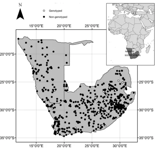
Figure 2. Geographic location of Rhabdomys occurrence records used in the analysis. Black dots indicate records of Rhabdomys obtained from various
sources (see Appendix 1) whereas open circles indicate genotyped individuals.
as a presence within a cell, whereas absence of any records was recorded as an absence. All environmental data were subse-quently processed to reflect this resolution. Aggregating these individual records into present records at the 10-km grid reso-lution resulted in 520 presence records for all Rhabdomys taxa. Among these records, 120 striped mice were assigned to a mitochondrial lineage based on published information of genotyped individuals (Rambau et al. 2003; Ganem et al. In Press). The numbers of presence records within the 10-km grid used in the analysis are shown in Table 1, and their spatial distribution in Figure 2.
Environmental data
Climate data and altitude were downloaded from the freely available Woldclim database (http://worldclim.org/). These data include climatic variables related to mean temperature and precipitation, as well as seasonality (see Appendix 1 for details), and were downloaded at a 30 arc-sec resolution (ap-proximately 1 km). The data were then converted to a 10-km resolution by using ArcGIS 9.2 focal mean functions.
A vegetation productivity index, the Enhanced Vegetation Index (EVI), as well as a land cover layer were downloaded from the Modis Terra website (http://modis.gsfc.nasa.gov/). Both layers were available at a 30 arc-sec resolution (ap-proximately 1 km). EVI is calculated by combining the near
Table 1. Number of grid cell records for the Rhabdomys lineages used in the statistical analysis. These correspond to the occurrences for
Rhabdomys (n= 6083) and the genotyped individuals (n = 120, taken from Rambau et al. 2003 and Ganem et al. In Press) summarized within each 10× 10 km grid cell as a presence (any number of records within the grid cell) or an absence (no records within that grid cell).
Clade Number of occurrences
Rhabdomys sp.* 520
Rhabdomys dilectus 21
Rhabdomys pumilio 30
Rhabdomys dilectus chakae 12
Rhabdomys dilectus dilectus 10
*Includes all striped mice identified morphologically as belonging to the genus.
infrared and red reflectance properties of vegetation to dis-criminate vegetation from other objects, and by reducing the influence of soil and atmospheric noise in the vegetation in-dex, generating a more reliable vegetation productivity index as compared for example to NDVI (Sims et al. 2006). Since EVI was available monthly, we downloaded 1 month repre-senting each austral season in 2004 (January, April, July, and October) and calculated the mean EVI values for each grid cell. We chose 2004 because data on land use were available for the same year, and this was an average year (no major heat wave or other extreme environmental event recorded). EVI was upscaled to 10-km resolution by using focal mean statistics.
Land use data were downloaded from the same source and processed using ArcGIS 9.2 to calculate the percent of each land use category in each 10× 10 km grid cell: in each 10-km grid cell, we calculated the percent covered by ever-green, deciduous, and mixed forests, closed and open shrub-land, woody and nonwoody savannas, grasslands, croplands, mixed crops and natural vegetation, urban areas, and barren or scarcely vegetated soil. The mean and range of all environ-mental variables considered are shown in Appendix 1. Statistical analysis
Characterization of environmental occupancy
All statistical analyses were carried out using R v2.8.1 (R Development Core Team 2005). In a first step, we needed to compare the actual occurrences of Rhabdomys and all lin-eages with the overall available information on the environ-ment in the study area. Since the number of grid cells without any records of Rhabdomys was much larger (roughly 19,500 grid cells) than the number of occupied cells in the study area (n= 520), doing so with the full dataset would have artifi-cially weighted absence records. Furthermore, those absences were both the result of no recorded individuals in a grid cell and the lack of visits to these areas. While different strate-gies to choose these pseudoabsences have been proposed in the literature (Phillips et al. 2009; VanDerWal et al. 2009; Warton and Shepherd 2010), we had to choose a pragmatic approach. Furthermore, species prevalence at around 50% has often been shown to produce better results in statisti-cal modeling (Fielding and Bell 1997; Reese et al. 2005). We therefore generated a dataset that contained all grid cells with records of Rhabdomys (n= 520), plus an equal number of randomly chosen grid cells with no records of Rhabdomys, and used this for the remainder of the statistical analysis. The dataset for the following statistical analyses therefore con-sisted of these 1040 grid cells, half of which contain presence records for the genus. The added pseudoabsences can be seen more appropriately as background data that will sample all the available environmental space rather than just the sites where Rhabdomys have been recorded (Phillips et al. 2009).
To characterize the environmental occupancy of each lin-eage, we carried out an Outlying Mean Index analysis (OMI) (Doledec et al. 2000). This is a multivariate analysis designed to study niche separation along environmental gradients and that has the advantage of considering linear as well as uni-modal relationships between species occurrence and environ-mental gradients (Doledec et al. 2000; Thuiller et al. 2004). The environmental gradients are summarized through an or-dination technique that looks for the optimal combination of environmental variables that separate species occurrences. We therefore carried out the OMI analysis in order to find the environmental gradients that best separate lineages in terms of their occurrence (Doledec et al. 2000), and we cal-culated the niche position (mean environmental conditions of occurrence) and niche breadth (variance around the niche position) of each lineage along each of the ordination axes (Thuiller et al. 2004). In order to test whether niche posi-tion and breadth for each lineage were significantly differ-ent from random, we randomly shuffled lineage occurrences within the environment and calculated the same statistics 1000 times. If the observed value of niche position and niche breadth was within the 2.5% lower or upper quantiles of dis-tribution of the randomizations (bootstrap two-tailed test), the observed value was considered as significantly different from random (Thuiller et al. 2004). We repeated the OMI analysis 10 times using different random samples to repre-sent the background environmental gradients, always finding consistent results. For simplicity, we only show results from one of those analyses.
Projecting potential distributions for each taxon
Since the number of occurrences in each taxon is fairly lim-ited, we could not use conventional statistical methods to project geographically the potential distributions of each clade. Instead, we used MAXENT (Phillips et al. 2006), a maximum entropy algorithm that has been shown to per-form fairly well even with a limited number of occurrences, and that can use presence-only data to project species poten-tial distributions (Elith et al. 2006). We therefore used this algorithm, along with the same environmental variables de-scribed above, in order to obtain potential distribution maps for Rhabdomys as a whole, as well as for the two species separately (R. pumilio and R. dilectus) and for each one of the proposed subspecies: R. d. chakae and R. d. dilectus. MAXENT results are presented as a relative suitability in-dex, where a higher value indicates a higher probability of occurrence of the species. To select a threshold above which the species will be considered as present, we used two dif-ferent methods: the Kappa maximization method and the maximization of the difference between sensitivity and speci-ficity, also known as Maximum Difference Threshold (MDT)
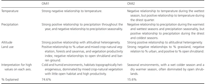
Table 2. Outlying Marginality Index (OMI) axes and their interpretation (details in Appendix 3). The general relationship to the environmental variables
used in the analysis are provided by category, then an overall interpretation of each axis is given, as well as the corresponding % variance explained by each axis.
OMI1 OMI2
Temperature Strong negative relationship to temperature. Negative relationship to temperature during the wettest season, but positive relationship to temperature during the driest quarter.
Precipitation Strong positive relationship to precipitation throughout the year, and negative relationship to precipitation seasonality.
Negative relationship to precipitation during the warmest and wettest seasons and precipitation seasonality, but positive relationship to precipitation during the driest and coldest seasons.
Altitude Strong positive relationship with altitudinal heterogeneity. Strong positive relationship to altitudinal heterogeneity. Land use Positive relationship to % urban and mixed crop-natural
veg-etation, forests and savannas, and vegetation productivity index; negative relationships to open shrubland and bar-ren ground.
Strong negative relationships to % grassland, negative relation to % urban, and positive to % open shrubland.
Interpretation for high values on each axis.
Cold and humid environments, habitats topographically het-erogeneous, dominated by mixed crop-natural vegetation with little open habitat and high productivity.
Seasonal environments, with a wet colder season and a dry warmer season, often dominated by open shrub-lands.
% Explained 74.6% 15.6%
(Liu et al. 2005; Jimenez-Valverde and Lobo 2007). These statistics were calculated on the random subset described above for the statistical analysis (n= 1040, including all pres-ences of Rhabdomys and a random subsample of abspres-ences where Rhabdomys prevalence was forced to be 50%). Perfor-mance of each model and each strategy are given in terms of sensitivity (success rate in predicting presences), specificity (success rate in predicting absences), and in terms of the Area Under the receiving operator Curve (AUC) that is indepen-dent of the threshold chosen and considers both presence and absence classification success rates (Fielding and Bell 1997).
Results
Characterization of environmental occupancy
The first two ordination axes, hereafter referred to as OMI1 and OMI2 respectively, explained 90 % of the niche separa-tion between taxa (Table 2 and Appendix 2). These ordinasepara-tion axes correspond to a combination of environmental variables that maximize the observed difference in the lineages’ oc-currences. The first axis represents the main environmental gradient explaining differentiation within Rhabdomys going from warm and dry habitats with low vegetation produc-tivity, to colder and more humid habitats with high vege-tation productivity although topographically heterogeneous (Table 2). The other ordination axis explained a lower pro-portion of the niche differentiation between lineages but still >15% (Table 2). OMI2 represents a gradient from less to more seasonal environments with a wet colder season and a
dry warmer season, and from grassland to open shrubland (Table 2 and Appendix 2).
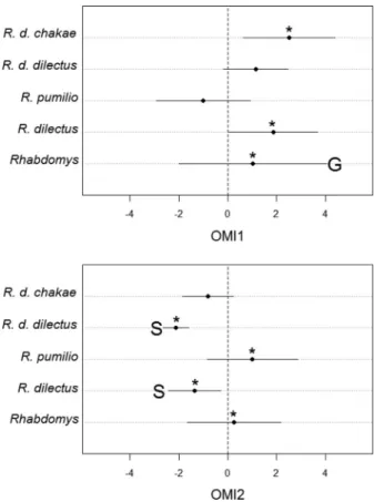
Rhabdomys as a genus shows a significantly wider niche breadth than expected by chance in the first OMI axis, and its niche is significantly different from 0 (i.e., differ-ent from mean available environmdiffer-ental conditions) in both axes (Fig. 3). Considering each species separately reveals dif-ferent occupancy requirements and patterns of specializa-tion within the genus. Rhabdomys dilectus shows significant positive values in niche position along OMI1 and both sig-nificant negative position and a narrower niche breath than expected by chance in OMI2 (Fig. 3). The two R. dilectus subspecies show only small differences: R. d. chakae, but not R. d. dilectus, shows a significantly positive niche position along OMI1, while R. d. dilectus, but not R. d. chakae, shows a significantly positive position and narrow niche breadth along OMI2. Rhabdomys pumilio niche position along OMI1 is negative but not significantly different from 0, while its position on OMI2 is significantly positive (Fig. 3).
Taken together these patterns support the idea that R. dilectus occurs in wet and relatively cold environments with a hot rainy season and a drier colder season supporting mixed crop-natural vegetation and grassland with little open habitat and high productivity (Table 2 and Fig. 3). On the other hand R. d. chakae occurs in more humid and colder environments than R. d. dilectus, the latter being found in warmer and more stable environments characterized by grassland-type vegeta-tion. In contrast to R. dilectus, environments occupied by R. pumilio appear to be more seasonal with a dry warm sea-son and a wet colder seasea-son, the vegetation being scarcer and more patchily distributed than where R. dilectus occurs.
Figure 3. Niche position and breadth along the first three
environmen-tal Outlying Mean Index (OMI) axes for each Rhabdomys lineage. Val-ues near 0 indicate environmental conditions near the available average conditions for that environmental gradient, whereas values far from this origin indicate marginal environments, that is, environments that are far from the environmental mean conditions. The asterisk indicates that the niche position is significantly different than that expected by random placement of the same number of occurrences (bootstrap two-tailed test, P< 0.05). S indicates that the niche breadth is significantly
nar-rower than expected by chance (S= specialist); G indicates that the taxon shows a significantly wider niche breath than expected by chance (G= generalist) (bootstrap two-tailed test, P < 0.05).
Projecting potential distributions for each taxon
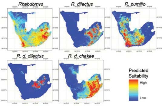
All projections show fairly high predictive success rates, with AUC often>0.9, the only exception being the projections for Rhabdomys as a genus (Table 3). Suitability maps pro-duced using MAXENT result in differential distributions for all taxa (Fig. 4). Using Kappa Maximizing Threshold (KMT) to determine the threshold for presence–absence predictions usually results in an excellent specificity (i.e., little error rate in absence predictions) but sometimes a poor sensitivity (i.e., a poor error rate in presence predictions) (Table 3). We there-fore present occurrence predictions based on MDT (Fig. 5), which resulted in a more balanced sensitivity and specificity (Table 3). Occurrence maps based on the KMT strategy are provided in Appendix 3. Under our prediction, R. pumilio presents the largest range as it occurs in the western (drier) part of the distribution range, but also penetrates further into the central part of southern Africa. While R. dilectus range appears to cover the eastern (wettest) part of southern Africa, with R. d. chakae occupying a larger area than R. d. dilectus, the latter being restricted to the northeastern part of our study area. Zones of overlap are predicted between the three taxa (Fig. 6).
Discussion
Museum collections provide a plethora of species occurrence data resulting from heterogeneous and often unknown sam-pling schemes. In parallel, accurate environmental data for large geographical areas are now available, providing pow-erful opportunities for zoologists aiming to gain a broader view on the distribution and ecological characteristics of their model taxa (Graham et al. 2004; Elith and Leathwick 2007). The present study has used these tools to assess environmental predictors of Rhabdomys distribution, to test whether envi-ronmental niche differentiation has occurred in a genus long
Table 3. Summary of model performance predicting species occurrences of Rhabdomys. Results are shown according to the threshold used to
determine species presence or absence from the suitability predicted by MAXENT. AUC, performance index; KMT, kappa maximizing threshold; MDT, maximum difference threshold. Notice that while AUC is threshold independent, sensitivity (presence prediction success rate) and specificity (absence prediction success rate) depend on the threshold chosen to predict occurrence from the continuous suitability index.
Threshold values KMT MDT
Taxon AUC KMT MDT Sensitivity Specificity Sensitivity Specificity
Rhabdomys 0.83 0.34 0.39 0.84 0.66 0.73 0.74
Rhabdomys dilectus 0.97 0.84 0.38 0.43 0.99 0.95 0.93
Rhabdomys pumilio 0.93 0.70 0.41 0.53 0.98 0.83 0.84
Rhabdomys dilectus chakae 0.91 0.78 0.57 0.17 0.99 0.92 0.86
Figure 4. Predicted suitability maps using MAXENT for all lineages of Rhabdomys.
Figure 5. Predicted distribution maps using MAXENT for all lineages of Rhabdomys based on maximum difference threshold (MDT) threshold (see
Methods for details and Appendix 3 for distribution maps based on KMT thresholds).
thought to be monospecific, and to predict where contact zones between its different taxa may occur. Patterns of envi-ronmental occupancy of Rhabdomys, as revealed in our study, indicate that historical considerations of the genus as a gener-alist (e.g., Skinner and Chimimba 2005) most probably result
from this rodent being a complex of taxa with different eco-logical characteristics. Furthermore, the two prerequisites for identifying secondary contact zones are (1) knowledge about the taxonomic identity of the taxa, and (2) characterization of the distribution range of each taxonomic entity. While
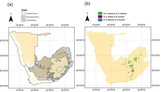
Figure 6. Predicted contact zones between lineages. Panel (a) shows the major biomes at the interface of contact zones in South Africa, as well as
the 900-m contour (yellow background) that constitutes an approximate limit for the escarpment area; panel (b) shows the actual predicted contact zones. These were drawn based on areas of overlap between the different lineages using MAXENT projections and a maximum difference threshold (MDT) to predict lineages occurrences (see Methods).
Rambau et al. (2003) and Castiglia et al. (2011) provided important taxonomic clarifications for Rhabdomys, we pro-vided here a thorough environmental characterization of the genus occupancy range that has not been attempted before, except at the much smaller scale of the Free State Province (Ganem et al. In Press). We therefore discuss these potential contact zones in more detail below.
Our results reveal at least two interesting aspects of the environmental occupancy patterns of Rhabdomys. First, dif-ferent taxa occupy difdif-ferent portions in the available envi-ronmental gradients. Only two envienvi-ronmental axes related to temperature and precipitation, and environmental vari-ability gradients (Table 2) explained a large portion of envi-ronmental differentiation between Rhabdomys taxa. These environmental variables have played a major role in the radiation of the genus (Rambau et al. 2003), and mirror previous suggestions that major biomes such as savannah and grasslands, which are greatly dependent on precipita-tion and temperature regimes, had major influences on the diversification of South Africa through their repeated ex-pansion and contraction during the Miocene and Pliocene (e.g., Daniels et al. 2006, 2009; Willows-Munro and Matthee 2011). This is also consistent with the Pliocene being a period of multiple episodes of aridification, resulting in landscape discontinuities over southern Africa (DeMenocal 2004), and which effected species diversification (Frey 1992; Lecompte
et al. 2008; Mirol et al. 2010; Russo et al. 2010). Second, environmental divergence within Rhabdomys parallels phy-logeny as the two species appear to be more distinct than the two subspecies. Rhabdomys pumilio occupies warmer, drier, and more seasonal environments and appears to be able to thrive in habitats with less cover and lower produc-tivity (e.g., the semidesert succulent Karoo) than R. dilectus. The two R. dilectus are always found in the same side of the environmental axes. Our results indicate that habitats where R. d. dilectus is found are characterized by grassland-type veg-etation and are warmer and less seasonal (e.g., Kwazulu-Natal midlands) than those of R.d. chakae that is characterised by both grassland and mixed crop-natural vegetation with high productivity index (e.g., northern parts of South Africa, ex-tending into Zimbabwe).
Fossil and paleoclimate information may help us pic-ture the original habitat of Rhabdomys ancestors. The ear-liest known Rhabdomys fossil was found in the southwestern coast of South Africa about 5 million years ago (Denys 1999 and references therein), suggesting that Rhabdomys ancestors thrived in a region where populations of R. pumilio still oc-cur today. Further, isotopic (δ13C) investigations in the fossil
site of Langebaanweg (Western Cape, SA) indicated that the region was probably a winter rainfall area characterized by a C3-type vegetation at that time (Segalen et al. 2007), as op-posed to C4-grassland-type vegetation in a mosaic landscape
of woodland patches described at an earlier period (4.0– 3.5 Ma) in the Free State (de Ruiter et al. 2010). The an-cestral habitat of Rhabdomys could therefore resemble that of the western range of the actual R. pumilio: a winter-fall region (WFR) mainly characterized by arid open-shrubland-type vegetation. Rhabdomys would have colonised the central and eastern regions only secondarily (unlike suggested by Rambau et al. 2003), possibly at a period when these re-gions had a different climate. Divergence within Rhabdomys occurred at dates similar to other rodents, such as the Namaqua rock mouse (Russo et al. 2010), and some inverte-brates (Daniels et al. 2006), supporting the links to climate cy-cles and consequent biome expansions and retractions lead-ing to population fragmentations and differentiation.
The distribution maps generated in this study reveal sev-eral potential contact zones and potential areas of localized sympatry along the sharp altitudinal gradient found in the southern tip of South Africa and the escarpment (e.g., the Cape Fynbos), in the grassland biome, as well as near its lim-its with the Nama Karoo and the savanna biome in the central part of South Africa (e.g., the Free State Province) (Fig. 6). As expected, given their relatively similar environmental charac-teristics, contact zones between the two R. dilectus subspecies, are predicted to cover large areas, mainly within the grass-land biome, with the only visible barrier being large urban areas of the Gauteng province, for example. However, sev-eral sites within this potential contact zone were visited and trapped and yielded only one or the other subspecies to date (Pillay et al. 2006 and subsequent unpubl. ms.). Further stud-ies are needed to confirm the absence of contact zones and disentangle the factors involved. Competition may be an im-portant ecological driver of species range boundaries in these areas where no obvious dispersal or habitat barrier exist and where the environment seems suitable for two subspecies but only one of them has been observed. Based on its pattern of mitochondrial divergence, Rambau et al. (2003) proposed that this subspecies show signs of recent expansion. It would therefore be interesting to use the contact zones map pro-duced here to investigate whether these areas are actually occupied by a single subspecies, possibly R. d. chakae, which would suggest that competitive replacement may occur be-tween the two subspecies.
Potential contacts between R. pumilio and the two R. dilec-tus subspecies occur mainly along a north to south axis near longitude 27◦E, with predictions of contact between the three taxa in the north of South Africa in edge regions of both the savannah and grassland biomes (Fig. 6). The contact zone between R. d. chakae and R. pumilio is also predicted to occur partly within the grassland biome, although in a region of important altitudinal heterogeneity close to the western part of the Drakensberg mountain range (Free State Province), the southern part of the escarpment, and down to the coastal area of Eastern Cape. In the southern part of this potential
con-tact zone, the Zuurberg Mountains could be separating these forms, with an additional change in vegetation from Nama Karoo to bushveld thicket. For the contact zone between R. d. dilectus and R. pumilio, there is no obvious physical bar-rier (as R. pumilio seems to have crossed the Orange River). The maps shown here predict this contact zone to occur within the grassland biome, which was confirmed by recent field work (Ganem et al. In Press).
Contact zones constitute candidate regions where future studies could investigate the extent of ecological divergence between the taxa (Fig. 6) (Rundle and Nosil 2005; Rissler and Smith 2010). Candidate areas of contact between the different lineages of Rhabdomys pinpointed in our study will allow effective targeting of field sites for further studies, al-lowing study of the current interplay between evolutionary and ecological mechanisms underlying speciation. For exam-ple, genetic divergence within Rhabdomys is also associated with behavioral divergence: high levels of aggression between lineages (Pillay 2000), divergence of the mate recognition system (Pillay et al. 2006), and regional differences in social organisation and reproduction (Schradin and Pillay, 2005b; Krug 2007). Differences in the behavior and ecology of the two main lineages described by Rambau et al. (2003) seem to be related to differences in population density, food availabil-ity (Schradin and Pillay 2005b; Schradin et al. 2010), and low nocturnal temperatures, resulting in the need for huddling in the desert (Scantlebury et al. 2006), factors that could all be influenced by prevailing climatic conditions and expected climate change. Overall, climate-dependent flexibility of be-havior could have been a key characteristic in the radiation of this genus (Schradin et al. 2011). Therefore, the study of these social and behavioral characteristics within and among the different lineages throughout their distribution range may help us understand the potential effects of future rapid envi-ronmental and climate change on these populations.
The maps of potential distributions for each taxon pro-posed here (Figs. 4 and 5; Appendix 3) can only be viewed as spatially explicit hypotheses of the distribution of each taxon. Indeed, the modeling effort carried out here presents some shortcomings linked to the limited number of occurrences used in the modeling process (Table 1). A minimum num-ber of 20–30 species occurrences has generally been recom-mended for use with MAXENT (Franklin 2009) and 50–70 occurrences are more generally recommended for species dis-tribution modeling (Stockwell and Peterson 2002; Wisz et al. 2008). However, MAXENT has been tested previously with very low occurrence numbers comparable to those used here, generating reasonably good distribution maps (Elith et al. 2006; Hernandez et al. 2006; Graham et al. 2010), and has generally been accepted as an appropriate tool for modeling species distributions when presence-only data are available (Elith et al. 2006). The lowest number of occurrences used here corresponds to R. d. dilectus, and is within the range of
occurrence records tested in Hernandez et al. (2006), sug-gesting that even under these circumstances, our predictions can be useful hypotheses of the distribution of the taxa.
Overall, our study pinpoints the urgent need to clarify the taxonomic status and distribution regarding different African taxonomic groups. Understanding the interplay between en-vironmental and ecological factors shaping large scale di-versity patterns requires a joint effort of this kind and is fundamental to providing realistic scenarios of biodiversity threats under climate change. We have provided here some hypotheses regarding the diversification of one rodent genus, Rhabdomys. However, our hypotheses could be validated if evidence from a diversity of taxonomic groups in the study region shows similar patterns. The identification of potential contact zones between the different taxa will also allow us to target future field and experimental work in order to tease apart the roles of ecological forces, such as competition, at in-terplay with evolutionary mechanisms, such as gene flow and hybridization between recently differentiated clades, in shap-ing species distribution boundaries, and in the maintenance of biodiversity.
Acknowledgments
We thank all the museums listed in Appendix 1 for sharing kindly their data with us. We thank Terri Bird for sharing Ar-cGIS shapefiles. This study is part of an international program of scientific collaboration financed by the NRF (South Africa) and the CNRS (France): PICS n◦4841. We have also benefited from financial and scientific support from the GDRI 191 and the University of the Witwatersrand. This is publication num-ber ISEM 2012-018.
References
Begon, M., J. L. Harper, and C. R. Townsend. 1996. Ecology, 3rd ed. Blackwell Science, Oxford, U.K.
Buckley, L. B. 2008. Linking traits to energetics and population dynamics to predict lizard ranges in changing environments. Am. Nat. 171:E1–E19.
Castiglia, R., E. Solano, R. H. Makundi, J. Hulselmans, E. Verheyen, and P. Colangelo. 2012. Rapid chromosomal evolution in the mesic four-striped grass rat Rhabdomys dilectus (Rodentia, Muridae) evaluated by mtDNA phylogeographic analysis. J. Zool. Syst. Evol. Res. DOI: 10.1111/j.1439-0469.2011.00627.x
Chen, I. C., J. K. Hill, H. J. Shiu, J. D. Holloway, S. Benedick, V. K. Chey, H. S. Barlow, and C. D. Thomas. 2011. Asymmetric boundary shifts of tropical montane Lepidoptera over four decades of climate warming. Global Ecol. Biogeogr. 20:34–45. Cruzan, M. B., and A. R. Templeton. 2000. Paleoecology and
coalescence: phylogeographic analysis of hypotheses from the fossil record. Trends Ecol. Evol. 15:491–496.
Daniels, S. R., G. Gouws, and K. A. Crandall. 2006. Phylogeographic patterning in a freshwater crab species (Decapoda: Potamonautidae: Potamonautes) reveals the signature of historical climatic oscillations. J. Biogeogr. 33:1538–1549.
Daniels, S. R., M. D. Picker, R. M. Cowlin, and M. L. Hamer. 2009. Unravelling evolutionary lineages among South African velvet worms (Onychophora: Peripatopsis) provides evidence for widespread cryptic speciation. Biol. J. Linn. Soc.
97:200–216.
De Graaff, G. 1981. The rodents of southern Africa. Butterworths, Pretoria, South Africa.
de Ruiter, D. J., J. K. Brophy, P. J. Lewis, A. M. Kennedy, T. A. Stidham, K. B. Carlson, and P. J. Hancox. 2010. Preliminary investigation of Matjhabeng, a Pliocene fossil locality in the Free State of South Africa. Palaeontol. Afr. 45: 11–22.
DeMenocal, P. B. 2004. African climate change and faunal evolution during the Pliocene-Pleistocene. Earth Planet. Sci. Lett. 220:3–24.
Denys, C. 1999. Of mice and men. Pp. 226–252 in T. G. Bromage and F. Schrenk, eds. African biogeography, climate change, and human evolution. Oxford Univ. Press, Oxford, U.K.
Doledec, S., D. Chessel, and C. Gimaret-Carpentier. 2000. Niche separation in community analysis: a new method. Ecology 81:2914–2927.
Elith, J., and J. Leathwick. 2007. Predicting species distributions from museum and herbarium records using multiresponse models fitted with multivariate adaptive regression splines. Diversity Distrib. 13:265–275.
Elith, J., and J. R. Leathwick. 2009. Species distribution models: ecological explanation and prediction across space and time. Annu. Rev. Ecol. Evol. Syst. 40:677–697.
Elith, J., C. H. Graham, R. P. Anderson, M. Dudik, S. Ferrier, A. Guisan, R. J. Hijmans, F. Huettmann, J. R. Leathwick, A. Lehmann, et al. 2006. Novel methods improve prediction of species’ distributions from occurrence data. Ecography 29:129–151.
Fielding, A. H., and J. F. Bell. 1997. A review of methods for the assessment of prediction errors in conservation
presence/absence models. Environ. Conserv. 24:38–49. Fjeldsa, J., E. Lambin, and B. Mertens. 1999. Correlation between
endemism and local ecoclimatic stability documented by comparing Andean bird distributions and remotely sensed land surface data. Ecography 22:63–78.
Franklin, J. 2009. Mapping species distributions: spatial inference and prediction. Cambridge Univ. Press, Cambridge, U.K.
Frey, J. K. 1992. Response of a mammalian faunal element to climatic changes. J. Mammal. 73:43–50.
Ganem, G., C. N. Meynard, M. Perigault, J. Lancaster, S. Edwards, P. Caminade, J. Watson, and N. Pillay. In Press. Presence of three mitochondrial lineages of striped mice (Rhabdomys) in the Free-State (South Africa): factors that may
promote their co-occurrence. Acta Oecol. DOI: 10.1111/j.1439-0469.2011.00627.x
Gaston, K. 2003. The structure and dynamics of geographic ranges, 1st ed. Oxford Univ. Press, Oxford, U.K.
Graham, C. H., S. Ferrier, F. Huettman, C. Moritz, and A. T. Peterson. 2004. New developments in museum-based informatics and applications in biodiversity analysis. Trends Ecol. Evol. 19:497–503.
Graham, C. H., N. Silva, and J. Velasquez-Tibata. 2010. Evaluating the potential causes of range limits of birds of the Colombian Andes. J. Biogeogr. 37:1863–1875.
Guisan, A., and W. Thuiller. 2005. Predicting species distribution: offering more than simple habitat models. Ecol. Lett.
8:993–1009.
Hernandez, P. A., C. H. Graham, L. L. Master, and D. L. Albert. 2006. The effect of sample size and species characteristics on performance of different species distribution modeling methods. Ecography 29:773–785.
Herzog, S. K., M. Kessler, and K. Bach. 2005. The elevational gradient in Andean bird species richness at the local scale: a foothill peak and a high-elevation plateau. Ecography 28:209–222.
Hijmans, R. J., S. E. Cameron, J. L. Parra, P. G. Jones, and A. Jarvis. 2005. Very high resolution interpolated climate surfaces for global land areas. Int. J. Climatol. 25:1965–1978.
Jimenez-Valverde, A., and J. M. Lobo. 2007. Threshold criteria for conversion of probability of species presence to either-or presence-absence. Acta Oecol.-Int. J. Ecol. 31:361– 369.
Krug, C. B. 2007. Reproduction of Rhabdomys pumilio in the Namib desert: pattern and possible control. Basic Appl. Dryland Res. 1:67–85.
Lecompte, E., K. Aplin, C. Denys, F. Catzeflis, M. Chades, and P. Chevret. 2008. Phylogeny and biogeography of African Murinae based on mitochondrial and nuclear gene sequences, with a new tribal classification of the subfamily. BMC Evol. Biol. 8:199.
Liu, C. R., P. M. Berry, T. P. Dawson, and R. G. Pearson. 2005. Selecting thresholds of occurrence in the prediction of species distributions. Ecography 28:385–393.
MacArthur, R. H. 1982. Geographical ecology: patterns in the distribution of species, 2nd ed. Princeton Univ. Press, Oxford, U.K.
Mirol, P., M. D. Gimenez, J. B. Searle, C. J. Bidau, and C. G. Faulkes. 2010. Population and species boundaries in the South American subterranean rodent Ctenomys in a dynamic environment. Biol. J. Linn. Soc. 100:368–383.
Moritz, C., C. J. Hoskin, J. B. MacKenzie, B. L. Phillips, M. Tonione, N. Silva, J. VanDerWal, S. E. Williams, and C. H. Graham. 2009. Identification and dynamics of a cryptic suture zone in tropical rainforest. Proc. R. Soc. B Biol. Sci.
276:1235–1244.
Nicolas, V. 2006. Mitochondrial phylogeny of African wood mice, genus Hylomyscus (Rodentia, Muridae): implications for their
taxonomy and biogeography. Mol. Phylogenet. Evol. 38:779–793.
Phillips, S. J., R. P. Anderson, and R. E. Schapire. 2006. Maximum entropy modeling of species geographic distributions. Ecol. Model. 190:231–259.
Phillips, S. J., M. Dudik, J. Elith, C. H. Graham, A. Lehmann, J. Leathwick, and S. Ferrier. 2009. Sample selection bias and presence-only distribution models: implications for background and pseudo-absence data. Ecol. Appl. 19:181– 197.
Pillay, N. 2000. Reproductive isolation in three populations of the striped mouse Rhabdomys pumilio (Rodentia, Muridae): interpopulation breeding studies. Mammalia 64:461–470. Pillay, N., J. Eborall, and G. Ganem. 2006. Divergence of mate
recognition in the African striped mouse (Rhabdomys). Behav. Ecol. 17:757–764.
Porzecanski, A. L., and J. Cracraft. 2005. Cladistic analysis of distributions and endemism (CADE): using raw distributions of birds to unravel the biogeography of the South American aridlands. J. Biogeogr. 32:261–275.
R Development Core Team. 2011. R: a language and environment for statistical computing. R Foundation for Statistical Computing. Vienna, Austria.
Rambau, R. V., T. J. Robinson, and R. Stanyon. 2003. Molecular genetics of Rhabdomys pumilio subspecies boundaries: mtDNA phylogeography and karyotypic analysis by fluorescence in situ hybridization. Mol. Phylogenet. Evol. 28:564–575.
Reese, G. C., K. R. Wilson, J. A. Hoeting, and C. H. Flather. 2005. Factors affecting species distribution predictions: a simulation modeling experiment. Ecol. Appl. 15:554–564.
Rissler, L. J., and W. H. Smith. 2010. Mapping amphibian contact zones and phylogeographical break hotspots across the United States. Mol. Ecol. 19:5404–5416.
Rowe, R. J., J. A. Finarelli, and E. A. Rickart. 2010. Range dynamics of small mammals along an elevational gradient over an 80-year interval. Global Change Biol. 16:2930–2943. Rundle, H. D., and P. Nosil. 2005. Ecological speciation. Ecol.
Lett. 8:336–352.
Russo, I. R. M., C. T. Chimimba, and P. Bloomer. 2010. Bioregion heterogeneity correlates with extensive mitochondrial DNA diversity in the Namaqua rock mouse, Micaelamys namaquensis (Rodentia: Muridae) from southern Africa – evidence for a species complex. BMC Evol. Biol. 10:307. Scantlebury, M., N. C. Bennett, J. R. Speakman, N. Pillay, and C.
Schradin. 2006. Huddling in groups leads to daily energy savings in free-living African four-striped grass mice
Rhabdomys pumilio. Funct. Eco. 20:166–173.
Schradin, C., and N. Pillay. 2005a. Intraspecific variation in the spatial and social organization of the african striped mouse. J. Mammal. 86:99–107.
Schradin, C., and N. Pillay. 2005b. Demography of the striped mouse (Rhabdomys pumilio) in the succulent karoo. Mammal. Biol. 70:84–92.
Schradin, C., B. K¨onig, and N. Pillay. 2010. Reproductive competition favours solitary living while ecological constraints impose group-living in African striped mice. J. Anim. Ecol. 79:515–521.
Segalen, L., J. A. Lee-Thorp, and T. Cerling. 2007. Timing of C-4 grass expansion across sub-Saharan Africa. J. Human Evol. 53:549–559.
Sims, D. A., A. F. Rahman, V. D. Cordova, B. Z. El-Masri, D. D. Baldocchi, L. B. Flanagan, A. H. Goldstein, D. Y. Hollinger, L. Misson, R. K. Monson, et al. 2006. On the use of MODIS EVI to assess gross primary productivity of North American ecosystems. J. Geophys. Res.-Biogeosci. 111:G04015. Skinner, J., and C. Chimimba. 2005. The mammals of the
southern African subregion. Cambridge Univ. Press, Cambridge, U.K.
Stockwell, D. R. B., and A. T. Peterson. 2002. Effects of sample size on accuracy of species distribution models. Ecol. Model. 148:1–13.
Thuiller, W., S. Lavorel, G. Midgley, S. Lavergne, and T. Rebelo. 2004. Relating plant traits and species distributions along bioclimatic gradients for 88 Leucadendron taxa. Ecology 85:1688–1699.
VanDerWal, J., L. P. Shoo, C. Graham, and S. E. William. 2009. Selecting pseudo-absence data for presence-only distribution modeling: how far should you stray from what you know? Ecol. Model. 220:589–594.
Warton, D. I., and L. C. Shepherd. 2010. Poisson point process models solve the "pseudo-absence problem" for presence-only data in ecology. Ann. Appl. Stat. 4:1383–1402.
Willows-Munro, S., and C. A. Matthee. 2011. Linking lineage diversification to climate and habitat heterogeneity: phylogeography of the southern African shrew Myosorex varius. J. Biogeogr. 38:1976–1991.
Wisz, M. S., R. J. Hijmans, J. Li, A. T. Peterson, C. H. Graham, and A. Guisan. 2008. Effects of sample size on the performance of species distribution models. Diversity Distrib. 14:763–773.
Appendix 1
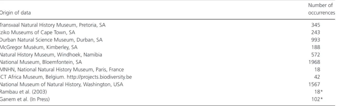
Summary of data used for the statistical analysis.Table A1 provides a summary of the various sources used to compile and georeference Rhabdomys records, while Table A2 provides a summary of environmental conditions in the study region including all environmental variables used as well as their mean and ranges.
Table A1. Summary of various sources used to georeference records of Rhabdomys sp.
Number of
Origin of data occurrences
Transvaal Natural History Museum, Pretoria, SA 345
Iziko Museums of Cape Town, SA 243
Durban Natural Science Museum, Durban, SA 993
McGregor Mus ´eum, Kimberley, SA 188
Natural History Museum, Windhoek, Namibia 572
National Museum, Bloemfontein, SA 1968
MNHN, National Natural History Museum, Paris, France 18 ICT Africa Museum, Belgium. http://projects.biodiversity.be 42 National Museum of Natural History, Washington, USA 1567
Rambau et al. (2003) 18*
Ganem et al. (In Press) 102*
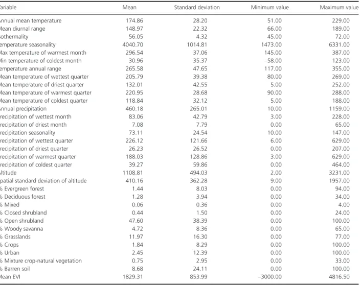
Table A2. Detailed description of environmental variables used in the statistical analysis for the distribution of Rhabdomys. Climatic variables were
downloaded from the freely available database Worldclim (www.worldclim.org). Climatic variable descriptions can be found in (Hijmans et al. 2005), and correspond to interpolated minimum, maximum, and mean values of temperature and precipitation gathered between 1950 and 2000. Notice that temperature is represented as temperature in◦C× 10, temperature seasonality corresponds to standard deviation of monthly data × 10, isothermality
corresponds to the ratio between diurnal and annual temperature range, and precipitation seasonality corresponds to the coefficient of variation of the monthly data. A vegetation productivity index, the Enhanced Vegetation Index (EVI), as well as land use were downloaded from Modis Terra. Land use categories were further transformed into percentage of each category within each 10× 10 km grid in our analysis.
Variable Mean Standard deviation Minimum value Maximum value Annual mean temperature 174.86 28.20 51.00 229.00 Mean diurnal range 148.97 22.32 66.00 189.00
Isothermality 56.05 4.32 45.00 72.00
Temperature seasonality 4040.70 1014.81 1473.00 6331.00 Max temperature of warmest month 296.54 37.06 145.00 387.00
Min temperature of coldest month 30.96 35.37 –58.00 123.00
Temperature annual range 265.58 47.65 117.00 355.00 Mean temperature of wettest quarter 205.79 39.38 80.00 269.00
Mean temperature of driest quarter 132.01 42.55 5.00 252.00
Mean temperature of warmest quarter 220.95 28.68 90.00 288.00
Mean temperature of coldest quarter 118.84 32.12 5.00 188.00
Annual precipitation 460.18 265.01 10.00 1159.00
Precipitation of wettest month 83.06 42.79 3.00 228.00
Precipitation of driest month 7.08 7.79 0.00 65.00 Precipitation seasonality 73.11 24.54 10.00 147.00
Precipitation of wettest quarter 226.12 121.66 6.00 629.00
Precipitation of driest quarter 26.23 26.52 0.00 207.00 Precipitation of warmest quarter 188.03 128.86 3.00 629.00
Precipitation of coldest quarter 39.27 59.86 0.00 464.00
Altitude 1108.81 494.03 2.00 3231.00
Spatial standard deviation of altitude 410.16 362.28 9.00 1957.00
% Evergreen forest 1.44 8.03 0.00 94.00 % Deciduous forest 1.28 3.94 0.00 34.00 % Mixed 0.06 0.36 0.00 4.00 % Closed shrubland 0.44 1.50 0.00 24.00 % Open shrubland 47.60 38.39 0.00 100.00 % Woody savanna 4.72 8.36 0.00 65.00 % Grasslands 11.97 16.30 0.00 77.00 % Crops 1.84 8.29 0.00 100.00 % Urban 2.45 12.39 0.00 100.00
% Mixture crop-natural vegetation 0.75 2.95 0.00 33.00
% Barren soil 8.68 24.11 0.00 100.00
Appendix 2
Details of Outlying Mean Index (OMI) analysis loadings. Each column represents the coefficients, that is, relative influence, of each variable for each OMI axis.
Variable OMI1 OMI2
Annual mean temperature −0.29 −0.06
Mean diurnal range −0.15 −0.05
Isothermality −0.10 −0.03
Temperature seasonality 0.00 0.00
Max temperature of warmest month −0.29 0.00
Min temperature of coldest month −0.20 0.04
Temperature annual range −0.08 −0.03
Mean temperature of wettest quarter −0.20 −0.15
Mean temperature of driest quarter −0.20 0.10
Mean temperature of warmest quarter −0.28 −0.03 Mean temperature of coldest quarter −0.25 −0.04
Annual precipitation 0.32 −0.07
Precipitation of wettest month 0.22 −0.12
Precipitation of driest month 0.26 0.09
Precipitation seasonality −0.24 −0.11
Precipitation of wettest quarter 0.23 −0.11
Precipitation of driest quarter 0.27 0.09
Precipitation of warmest quarter 0.29 −0.13
Precipitation of coldest quarter 0.15 0.15
Altitude 0.10 −0.10
Spatial standard deviation of altitude 0.20 0.17
% Evergreen forest 0.11 0.06 % Deciduous forest 0.10 0.03 % Mixed 0.07 0.03 % Closed shrubland 0.06 0.05 % Open shrubland −0.19 0.12 % Woody savanna 0.09 −0.04 % Grasslands 0.07 −0.18 % Crops 0.10 0.07 % Urban 0.21 −0.12
% Mixture crop-natural vegetation 0.17 −0.03
% Barren soil −0.11 0.04
Appendix 3
Distribution maps generated using the maximum kappa (KMT) threshold criteria for the different lineages of Rhabdomys (see Methods).