HAL Id: hal-00297666
https://hal.archives-ouvertes.fr/hal-00297666
Submitted on 28 Jan 2008
HAL is a multi-disciplinary open access
archive for the deposit and dissemination of
sci-entific research documents, whether they are
pub-lished or not. The documents may come from
teaching and research institutions in France or
abroad, or from public or private research centers.
L’archive ouverte pluridisciplinaire HAL, est
destinée au dépôt et à la diffusion de documents
scientifiques de niveau recherche, publiés ou non,
émanant des établissements d’enseignement et de
recherche français ou étrangers, des laboratoires
publics ou privés.
with a mechanistic model to estimate nitrogen and
carbon losses from arable soils in Europe
A. Leip, G. Marchi, R. Koeble, M. Kempen, W. Britz, C. Li
To cite this version:
A. Leip, G. Marchi, R. Koeble, M. Kempen, W. Britz, et al.. Linking an economic model for European
agriculture with a mechanistic model to estimate nitrogen and carbon losses from arable soils in
Europe. Biogeosciences, European Geosciences Union, 2008, 5 (1), pp.73-94. �hal-00297666�
www.biogeosciences.net/5/73/2008/ © Author(s) 2008. This work is licensed under a Creative Commons License.
Biogeosciences
Linking an economic model for European agriculture with a
mechanistic model to estimate nitrogen and carbon losses from
arable soils in Europe
A. Leip1, G. Marchi1, R. Koeble1,*, M. Kempen2, W. Britz2,1, and C. Li3
1European Commission – DG Joint Research Centre, Institute for Environment and Sustainability, Ispra, Italy
2University of Bonn, Institute for Food and Resource Economics, Bonn, Germany
3Institute for the Study of Earth, Oceans, and Space, University of New Hampshire, Durham, NH 03824, USA
*now at: Institute of Energy Economics and the Rational Use of Energy, Department of Technology Assessment and
Environment, Stuttgart, Germany
Received: 23 May 2007 – Published in Biogeosciences Discuss.: 5 July 2007
Revised: 10 October 2007 – Accepted: 2 December 2007 – Published: 28 January 2008
Abstract. A comprehensive assessment of policy impact on greenhouse gas (GHG) emissions from agricultural soils re-quires careful consideration of both socio-economic aspects and the environmental heterogeneity of the landscape. We developed a modelling framework that links the large-scale economic model for agriculture CAPRI (Common Agricul-tural Policy Regional Impact assessment) with the biogeo-chemistry model DNDC (DeNitrification DeComposition) to simulate GHG fluxes, carbon stock changes and the nitrogen budget of agricultural soils in Europe. The framework allows the ex-ante simulation of agricultural or agri-environmental policy impacts on a wide range of environmental problems such as climate change (GHG emissions), air pollution and groundwater pollution. Those environmental impacts can be analyzed in the context of economic and social indicators as calculated by the economic model. The methodology con-sists of four steps: (i) definition of appropriate calculation units that can be considered as homogeneous in terms of eco-nomic behaviour and environmental response; (ii) downscal-ing of regional agricultural statistics and farm management information from a CAPRI simulation run into the spatial calculation units; (iii) designing environmental model sce-narios and model runs; and finally (iv) aggregating results for interpretation. We show the first results of the nitrogen bud-get in croplands in fourteen countries of the European Union and discuss possibilities to improve the detailed assessment of nitrogen and carbon fluxes from European arable soils.
Correspondence to: A. Leip (adrian.leip@jrc.it)
1 Introduction
Agricultural activity is responsible for environmental con-cern, causing among others elevated nitrate concentrations in water, emitting ammonia into the atmosphere and contribut-ing to increase GHG concentrations in the atmosphere. The source strength of these pollutants must be assessed both un-der international obligations and European legislation. Rec-ommended procedures for the estimation of GHG emissions (IPCC, 1997; 2000; 2006; EMEP/CORINAIR 2003) have a large uncertainty range. In addition, they lack the ability to differentiate regional conditions and accommodate mit-igation measures. Therefore the development of reliable, independent and flexible assessment tools is needed (i) to assess the response of the environmental system to socio-economically driven pressures, while reflecting the various feedbacks and interactions between natural drivers, (ii) to consider regional differences in the response in order to (iii) finally find regionally stratified emission factors or emission
functions. Process-based models can be used for
report-ing GHG emissions from agricultural soils under the United Nations Framework Convention on Climate Change (Leip, 2005). Such models are adequate to analyze the impact of changing farming practices, as they are able to simulate com-plex interactions occurring between the environment and an-thropogenic activities, but a successful application from the regional to the continental scale depends on matching agri-cultural activities with the environmental circumstances (Liu et al., 2006; Mulligan, 2006) and on the quality of the input data. The accuracy of simulating fluxes with process-based models such as the DNDC (Denitrification Decomposition) Model (Li et al., 1992), for example, has been shown to be especially sensitive to soil organic matter (SOM) content and
nitrogen fertilizer application rates. As the response of pro-cess based models to climate and soil parameters or agricul-tural management is non-linear, their application to regional averages of those input data leads to aggregation bias. Re-sulting uncertainties of a factor of 10 or more are common (Mulligan, 2006).
A comprehensive assessment of emissions from arable soils needs to consider the feedbacks between livestock pop-ulation and cropland areas via fodder production or between stocking densities and manure application rates. Such feed-backs are inherent in large scale economic models such as CAPRI, which capture the complex interplay between the market, environmental policies and the economic behaviour of the different agents (farmers, consumers, processors) from global to regional scale.
Examples of policy-related process studies for agriculture at the continental scale exist for carbon sequestration (e.g. Smith et al., 2005b), nitrogen oxide emissions from forest soils (e.g. Kesik et al., 2005), investigating different manage-ment practices (e.g. Grant et al., 2004), or assessing global change scenarios (Schr¨oter et al., 2005). Examples for stud-ies regarding livestock systems can be found for dairy farm-ing (Weiske et al., 2006) or grassland systems (Soussana et al., 2004). Integrated multi-sectoral modelling systems (eg. IMAGE, Bouwman et al., 2006; RAINS, H¨oglund-Isaksson et al., 2006) are limited to relatively simple parameterizations of pollutant fluxes. There are only a few examples where an overall assessment is achieved through linking economic with process-based models (e.g. Neufeldt et al., 2006; Wat-tenbach et al., 2007), but the area of interest is much smaller than in the present study.
This paper focuses on the methodology developed to link the large-scale regionalised economic model CAPRI to the biophysical DNDC model in order to develop a new policy impact simulation tool for the area of the European Union. The tool allows the ex-ante simulation of agricultural or agri-environmental policy impacts on a wide range of environ-mental problems such as climate change (GHG emissions), air pollution and groundwater pollution. The analysis of the trade-off between the different pillars of sustainability of such policies is inherently built into the policy tool. The ob-jectives of the present study are therefore (i) to give a detailed description the CAPRI/DNDC-EUROPE framework, includ-ing the agricultural land use map, that serves as an important element in linking both models and (ii) to critically examine the quality of the data sets that are available to drive process-based models at the continental scale in Europe.
2 Methods
2.1 Models
2.1.1 DNDC
The DNDC model predicts biogeochemistry in, and fluxes of carbon and nitrogen from agricultural soils. DNDC was developed in 1992 and since then has had ongoing enhance-ments (Li, 2000; Li et al., 1992, 2004, 2006). DNDC is a biogeochemistry model for agro-ecosystems that can be ap-plied both at the plot-scale and at the regional scale. It con-sists of two components. The first component calculates the state of the soil-plant system such as soil chemical and phys-ical status, vegetation growth and organic carbon mineral-ization, based on environmental and anthropogenic drivers (daily weather, soil properties, farm management). The sec-ond component uses the information on the soil environment to calculate the major processes involved in the exchange of GHGs with the atmosphere, i.e. nitrification, denitrification and fermentation. The model thus is able to track production, consumption and emission of carbon and nitrogen oxides, ammonia and methane. The model has been tested against
numerous field data sets of nitrous oxide (N2O) emissions
and soil carbon dynamics (Li et al., 2005).
DNDC has been widely used for regional modelling stud-ies in the USA (Tonitto et al., 2007), China (Li et al., 2006; Xu-Ri et al., 2003), India (Pathak et al., 2005) and Europe (Brown et al., 2002; Butterbach-Bahl et al., 2004; Neufeldt et al., 2006; Sleutel et al., 2006). The simulations reported here were done with a modified version of DNDC V.89, al-lowing a more flexible simulation of a large number of pixel-clusters. These modifications enabled us to simulate an un-limited number of agricultural spatial modelling units with individual farm and crop parameterization and with the op-tion to individually select up to ten different crops to be sim-ulated within a specific calculation unit.
2.1.2 CAPRI
The agricultural economic model CAPRI sets a framework based on official national and international statistics, the global agricultural market and trade systems, and the agri-cultural policy environment and responses of agents (farm-ers, consum(farm-ers, processors) to changes in policies and mar-kets. The main purpose of CAPRI is the Pan-European ex-ante policy impact assessment from regional to global scale. Policies considered include premiums paid to farmers, bor-der protection by tariffs, and agri-environmental legislation. CAPRI is operationally installed at the European Commis-sion and has been used in a wide range of studies and re-search projects, e.g. in a recent study by DG-Environment on ammonia abatement measures. In this study we use aver-aged data of the years 2001–2003. A detailed description of the CAPRI modelling system is given in Britz (2005).
Socio-economic database Socio-economic database DNDC DNDC European national and international statistics European national and international statistics
GIS environmental database GIS environmental database
CAPRI CAPRI Regional statistics Regional statistics National market/trade Regional agricultural system + economic and environmental indicators Policy framework Policy framework Global trade framework Global trade framework
Production level and farm input estimation at spatial calculation units
Agricultural land use map Agricultural land use
map Definition of
environmental scenario
Aggregation to modeling spatial units
Climate data and N deposition Soil information DNDC-EUROPE Farm Management Farm Management Simulation at modeling spatial unit Environmental indicators - N2O, N2 - NOx - CH4 - NH3 - Nitrate leaching - Carbon Stocks - Livestock density - … Environmental indicators - N2O, N2 - NOx - CH4 - NH3 - Nitrate leaching - Carbon Stocks - Livestock density - … Geographic data
Fig. 1. Flow-diagram of the CAPRI-DNDC-EUROPE framework. The modelling framework aims also at depicting the flow of nutrients through the production systems. Improvements on some elements have been achieved in the present study, as described below, and a spatial layer was added.
2.1.3 CAPRI DNDC-EUROPE model link
We combine a socio-economic database, defined at the level of administrative regions and designed to drive the economic model CAPRI, and an environmental database in a Geo-graphical Information System (GIS) environment, which is mainly used to drive the process-based model DNDC. The environmental database also contains agricultural land use and livestock density maps, which are derived using econo-metric methodologies as described in Sect. 2.3. Environ-mental and land use/management information are used to-gether with the estimates of production levels and farm input (see Sect. 2.4.1) at the scale of the spatial calculation units, which are obtained within the CAPRI modelling framework, to define the scenario and set-up the aggregation level and final input database to run the DNDC model (Sect. 2.6). An overview of the link between the two models is given in Fig. 1. The set of environmental indicators contains both data on soil fluxes calculated with the process-based model and emissions from livestock production systems.
2.2 The spatial calculation unit
The smallest unit at which agricultural statistics for EU Member States are available are the so-called Nomenclature of Territorial Units for Statistics (NUTS) regions level two or three, which correspond to administrative areas of 160 km2to
440 km2(NUTS2) or 32 km2to 165 km2(NUTS3). Areas of
this size span a wide range of natural conditions: soil type, climate and also landscape morphology. We chose four de-limiters to define a spatial calculation unit, denoted as “Ho-mogeneous Spatial Mapping Unit” (HSMU), i.e. soil, slope, land cover and administrative boundaries. The HSMU is re-garded as similar both in terms of agronomic practices and the natural environment, embracing conditions that lead to similar emissions of GHGs or other pollutants.
The HSMUs were built from four major data sources, which were available for the area of the European Union, i.e. the European Soil Database V2.0 (European Commis-sion, 2004) with about 900 Soil Mapping Units (SMU), the CORINE Land Cover map (European Topic Centre on Terrestrial Environment, 2000), administrative boundaries (EC, 2003; Statistical Office of the European Communities (EUROSTAT), 2003), and a 250 m Digital Elevation Model (CCM DEM 250, 2004). Prior to further processing, all maps were re-sampled to a 1 km raster map (ETRS89 Lambert Az-imuthal Equal Area 52N 10E, Annoni, 2005) geographically consistent with the European Reference Grid and Coordinate Reference System proposed under INSPIRE (Infrastructure for Spatial Information in the European Community, Com-mission of the European Communities, 2004).
One HSMU is defined as the intersection of a soil map-ping unit, one of 44 CORINE land cover classes, adminis-trative boundaries at the NUTS 2 or 3 level and the slope according to the classification 0◦, 1◦, 2–3◦, 4–8◦and >8◦. As the HSMU of at least two single pixel of one square km are not necessarily contiguous, we can speak of the HSMU as a “pixel cluster”.
2.3 Estimating agricultural production
2.3.1 Crop levels
Statistical information about agricultural production was obtained at the regional NUTS 2 level from the CAPRI
database. This database contains official data obtained
from the European statistical offices (available at http:// epp.eurostat.ec.europa.eu) and has been checked for com-pleteness and inherent consistency and complemented with management data to make them useful for modelling pur-poses (Britz et al., 2002).
Data on crop areas are downscaled to the level of the HSMU using a two-step statistical approach combining prior estimates based on observed behaviour with a reconciliation procedure achieving consistency between the scales (Kem-pen et al., 2007).
The first step develops statistical regression models to es-timate the probability that a crop is grown in an HSMU as a function of environmental characteristics (climate, soil properties, land cover, etc.). The model parameters are cal-ibrated with observational data from the Land Use/Cover Area Frame Statistical Survey (LUCAS, European Commis-sion, 2003). To account for the possibility that factors other than natural conditions influence the choice of farmers to grow a specific crop, the weight of LUCAS observations is discounted with the distance from the respective HSMUs (Locally Weighted Binomial Logit Models, e.g. Anselin et al., 2004). Based on these parameters the first and second moments of a priori estimates of the land use shares are cal-culated for each HSMU and for each of the 29 crops for which statistical information is available.
In the second step consistency with the regional statistics is then obtained with a Bayesian Highest Posterior Density (HDP) estimator. The final results are (with respect to the a priori information) the most probable combination of crop-ping shares at HSMU level which exhaust the agricultural area of each HSMU and are in line with given regional crop and land use data or projections.
The area under analysis covers 25 Member States of the European Union; Malta and Cyprus are not included. As ex-plained above, land cover is one of the delineation factors for the HSMUs which allowed exclusions of such HSMUs where we assumed that no agricultural cover should be present. However, a rather wide range of land cover classes comprising 11 agricultural or mixed agricultural CORINE land cover classes and 7 non-agricultural classes was main-tained. As the definition of a CORINE mapping unit re-quires a minimum of 25 ha of homogeneous land cover, spa-tial units might include fractions of other CORINE classes, e.g. it is typical to find some grassland in forest areas and vice versa. In regions with predominantly forest land cover, significant percentages of grassland reported in agricultural statistics might be “hidden” in CORINE forest classes while in regions with prevailing “pasture” according to CORINE
this share might be negligible. The overall procedure tries to eliminate these negligible fractions of land use from the HSMU by manipulating the prior expectations.
2.3.2 Estimating animal stocking densities
Manure availability is linked to livestock density and we as-sume a close link between local manure availability and local application rates. Unlike crops, there is no common Pan-European data base available with high spatial resolution data on animal herds, necessary for the estimation of local parameter sets of regression functions for animal stocking densities. Instead, data on herd sizes from the Farm Struc-ture Survey (FSS) at NUTS 2 or 3 level (about 1 000 re-gions for EU25) were regressed against data which are avail-able or can be estimated at the level of single HSMUs: crop shares, crop yields, climate, slope, elevation and economic indicators for group of crops as revenues or gross margins per hectare. All explanatory variables are offered in linear and quadratic form as well as square roots to an estimator which uses backward elimination. Generally the estimation is done per single Member State; however, in cases where not enough FSS regions are available for a Member State, countries are grouped during the estimation. The regression is applied to the 14 animal activities covered in the CAPRI data base as well as for livestock aggregates (ruminants, non-ruminants and all types of animals) on the basis of livestock units (LUs). The vast majority of the regressions yield
ad-justed R2above 80%. As expected, a low share of explained
variance was found in a number of cases for area independent livestock systems (pigs, poultry).
Because the variance of explanatory variables at the HSMU level is far greater than in the FSS region sample per Member States, estimating at a single HSMU level would be prone to yield outliers with a high variance of forecast er-ror. The forecast for stocking densities of different animals per HSMU were therefore obtained by using a distance- and size-weighted average of the explanatory variables of the sur-rounding HSMUs. As for crops, the forecasts per HSMU must recover the herds at the NUTS 2 level to yield con-sistent downscaling. In order to do so, a Highest Posterior Density estimator was used, which corrects the forecasts to match the regional herds, taking into account the variance of the forecast error when determining the correction factor per HSMU and animal type.
2.3.3 Potential yield
DNDC simulates the crop growth at a daily time step, using a pre-defined logistic function (S-curve) representing a tra-jectory to maximum obtainable nitrogen uptake and biomass carbon. Partitioning total biomass into the plant’s compart-ments (root, shoot, grain) at harvesting time is also given as default data in the crop library files (Li et al., 2004). In the absence of any limiting factors (nitrogen, soil water,
radiation, etc.) the pdefined total plant carbon will be re-alized at harvest time. If any stress of temperature, water or nitrogen occurs during the simulated crop-growing season, a reduction of the biomass will be quantified by DNDC. In-formation of potential yields for soil polygons was obtained from the JRC crop growth monitoring system (Genovese et al., 2007). This was used to down-scale statistical production data at the regional level in CAPRI to the scale of HSMUs.
2.4 Estimating agricultural management
The DNDC model requires the following agricultural man-agement parameters: application rates and timing of mineral and organic fertilizer, tillage timing and technique, irrigation, sowing and harvesting dates. Additional data, such as infor-mation on crop phenology, are optional.
2.4.1 Calculation of mineral and organic fertilizer
applica-tion rates
Estimation of nitrogen application rate per crop at HSMU level is based on a spatial dis-aggregation of estimated appli-cation rates at the regional (NUTS 2) level from the CAPRI regional data base. As there are no Pan-European statistics on regional application rates available, the estimation process in CAPRI at the NUTS 2 level is briefly described. The chal-lenge is to define application rates that are consistent with given boundary data – national mineral fertiliser use and ma-nure nitrogen excreted from animals – cover crop needs, and lead to a plausible distribution of nitrogen losses over crops and regions. The estimation is based on the Highest Poste-rior Density Estimator. Manure nitrogen in a region is de-fined as the difference between nitrogen intake via feed – ei-ther concentrates or regionally produced fodder – and nitro-gen removals by selling animal products according to a farm-gate balance approach. Assuming no trade of nutrients across NUTS 2 boundaries, the available organic nitrogen must be exhausted by the estimated organic application rates. The same holds at the national level for total mineral nitrogen use in agriculture. Estimates at the Member State level on min-eral application rate for selected crops or groups of crops are available from the International Fertilizer Manufacturers Or-ganization (FAO/IFA/IFDC/IPI/PPI, 2002) which also pro-vides statistics on total mineral fertilizer use in agriculture. The HDP estimator is set up as to minimize simultaneously the differences between the estimated and given national ap-plication rates and to stay close to typical shares of crop needs covered by organic nitrogen and assumed regional sur-pluses, ensuring via constraints that crop needs are covered and the available mineral and organic nitrogen is distributed. Upper bounds on organic application rates reflecting the Ni-trate Directive are introduced for NUTS 2 regions comprising nitrate vulnerable zones.
At the HSMU level, nitrogen removals per crop are defined from the estimated crop yields. In order to determine manure
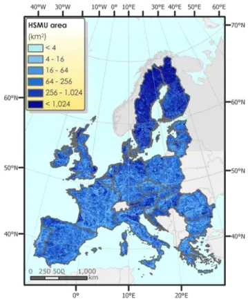
Fig. 2. Size distribution of homogeneous spatial mapping units with CCM 250 DEM hillshade.
organic application rates per crop and HSMU, we first esti-mate average manure application rate per crop for the NUTS 2 regions surrounding the HSMU, using the inverse distance in kilometre multiplied with the size of NUTS 2 region in square kilometre as weights. The same weights are used to define the average organic nitrogen available per hectare in the regions surrounding the HSMU. The manure application rate per crop in each HSMU is obtained by the multiplication of three terms, i.e. (i) the average organic application rate in the surrounding regions as defined above; (ii) the relation between the crop specific nitrogen removal at HSMU yield and the removal at NUTS 2 yield; and (iii) a term depending on the relation between the organic nitrogen availability per hectare at HSMU level, which is obtained from animal stock-ing density in the HSMU, the average manure availability as described above, and the size of the HSMU. The resulting es-timated crop specific organic application rates per crop and HSMU are scaled with a uniform factor to match the given regional application rates. Summarizing, organic rates at the HSMU level will exceed average NUTS 2 rates if yields are higher – leading to higher nitrogen crop removal – or if stock-ing densities are higher – drivstock-ing up organic nitrogen avail-ability.
Mineral application rates are calculated as the difference between crop removals plus the relative surplus estimated at regional level minus the estimated application rate of manure
nitrogen. Ammonia losses and atmospheric deposition are taken into account. Those estimates are increased in cases that assumed minimum application rates are not reached. As with organic rates, a uniform scaling factor lines up the HSMU-specific estimates with the regional ones.
2.4.2 Field management
Crop sowing and harvesting dates are obtained from Bouraoui and Aloe (2007). Scheduling of crop management is calculated by applying pre-defined time lags between crop sowing and tillage or fertilizer applications. These are ob-tained from the DNDC farm library (Li et al., 2004). Irriga-tion is treated in the DNDC model such that a calculated wa-ter deficit is replenished whenever it occurs. Irrigated crops do not suffer any water deficit while non-irrigated cultiva-tions will endure water-stress when water demand by the plants exceeds water supply. The percentage of irrigated area was calculated on the basis of the map of irrigated ar-eas (Siebert et al., 2005) and was taken as fixed for all crops being cultivated within a HSMU.
2.4.3 Other management data
All other information needed to describe farm management and crop growth, such as tillage technique, maximum rooting depth and so on, are taken from the DNDC default library and used as a constant for each crop for the entire simulated area.
2.5 Environmental input data
2.5.1 Nitrogen deposition
Data on nitrogen concentration in precipitation were ob-tained from the Co-operative Programme for the Monitoring and Evaluation of the Long-Range Transmission of Air Pol-lutants in Europe (EMEP, 2001). EMEP reports the data as
precipitation weighted arithmetic mean values in mg N L−1
as ammonium and nitrate measured at one of the permanent EMEP stations. We used the European coverage processed by Mulligan (2006).
2.5.2 Weather data
Daily weather data for the year 2000 were obtained from the Joint Research Centre (Institute for Protection and Security of the Citizen). The data originate from more than 1 500 weather stations across Europe, which were spatially inter-polated onto a 50 km×50 km grid by selecting the best com-bination of meteorological stations for each grid (Orlandi and Van der Goot, 2003).
2.5.3 Soil data
The DNDC model requires initial content of total soil or-ganic carbon (SOC) data in kg C kg−1of soil, including litter residue, microbes, humads and passive humus in the topsoil
layer, clay content (%), bulk density (g cm−3)and pH. Such
data were obtained from a series of 1 km×1 km soil raster data sets that were processed on the basis of the European
Soil Database1(Hiederer et al., 2003). Data on packing
den-sity and base saturation had been used by Mulligan (2006) to obtain dry bulk density and pH, respectively, using linear relationships. Soil organic carbon content was derived using an extended CORINE land cover dataset, a Digital Eleva-tion Model and mean annual temperature data (Jones et al., 2005). As DNDC has been parameterized for mineral soils, we restricted the simulations to spatial units with a topsoil organic content of less than 200 t ha−1(Smith et al., 2005a). These data were used to initialize soil characteristics and soil carbon pools by means of a 98 year spin-up run.
2.6 Model set-up
The above-defined HSMU can be regarded as the smallest
unit on which simulations can be carried out. However,
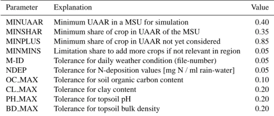
the practicality of this is compromised by the large num-ber of units and scenarios, and more so when a multi-year simulation is carried out. Therefore, an intermediate step re-aggregates similar HSMUs into Model Simulation Units (MSUs) on the basis of both agronomic and environmental criteria. In this way the design of the scenario calculations can better fit the objectives of the study. Within one MSU, the variability of environmental characteristics is kept at a minimum on the basis of pre-defined tolerances (Table 1). The HSMUs were regarded as similar if topsoil organic mat-ter content differed by less than ±10% and clay content, pH and bulk density by less than ±20%. The table shows also the threshold values for the minimum percentage of agricul-tural area and the minimum crop share, as well as additional thresholds ensuring that all significant agricultural activities are included in the simulations. These moderate tolerances and thresholds led to an average of more than 68 (up to 266) different soil conditions that were distinguished in each re-gion, which translates to 11 438 environmental situations for EU15, out of which 6 391 MSU were simulated with a total of 11 063 crop-MSU combinations.
We had complete information for 14 European countries that were members of the European Union in 2004: Austria, Belgium, Finland, France, Germany, Greece, Luxembourg (simulated as part of Belgium), Italy, Netherlands, Portugal, Spain, Sweden, and United Kingdom. Statistical and weather information were centred on the year 2000. HSMU data for Ireland and the countries that joined the European Union in 2004 or 2007 have also been processed but are not yet in-cluded in the current simulation run. We simulated the fol-lowing crops: cereals (soft and durum wheat, barley, oats, rye, maize and rice), oil seeds (rape and sunflower),
legumi-1Distribution version 2.0, http://eusoils.jrc.it/ESDB Archive/ ESDB/index.htm
Table 1. Thresholds and tolerances used to cluster HSMUs into MSUs and to select the simulated crops.
Parameter Explanation Value
MINUAAR Minimum UAAR in a MSU for simulation 0.40
MINSHAR Minimum share of crop in UAAR of the MSU 0.35
MINPLUS Minimum share of crop in UAAR not yet considered 0.85
MINMINS Limitation share to add more crops if not relevant in region 0.05
M-ID Tolerance for daily weather condition (file-number) 0.05
NDEP Tolerance for N-deposition values [mg N / ml rain-water] 0.05
OC MAX Tolerance for soil organic carbon content 0.10
CL MAX Tolerance for clay content 0.20
PH MAX Tolerance for topsoil pH 0.20
BD MAX Tolerance for topsoil bulk density 0.20
Fig. 3. (a) UAAR (b) Livestock density in EU27, superimposed on a hill-shade.
nous crops (soybean, pulses), sugar beets, potatoes, vegeta-bles and fodder production on arable land.
Each scenario was calculated under irrigated and non-irrigated conditions and the two simulations weighted
ac-cording to the irrigation map. Simulation results were
aggregated to the scale of the regions or countries as area-weighted averages.
3 Results
3.1 Homogeneous spatial mapping units
The HSMUs span a wide range of sizes from a minimum
area of 1 km2 to some very large areas (up to 9 723 km2)
in regions with a homogeneous landscape in terms of land cover and soil. The mean area of a HSMU indicates the range of environmental diversity with regard to land cover,
administrative, data, soil and slope, and ranges from 7 km2
for Slovenia to 94 km2 for Finland with an European
aver-age around 21 km2(see Table 2 and Fig. 2). In total, 206 000
HSMUs covering almost 4.3 million km2in Europe were
de-fined. Small discrepancies in the surface area of countries stem from rounding errors during the re-sampling procedure and are higher in areas with a high geographical fragmenta-tion (e.g. small islands, complex coastlines or borders). For EU27 we obtained in total about 138 000 HSMUs in which agricultural activities (arable land and grassland) occur, oc-cupying about 77% of the European landscape.
Table 2. Main statistics on the layer of the homogeneous spatial mapping units (HMSUs) for EU27 without Malta and Cyprus.
Country Number Total Area Mean Size Number Mean Size Total Area Mean UAAR Total UAAR [n] [1000 km2] [km2] [n] [km2] [1000 km2] [%] [1000 km2]
ALL HSMUs HSMUs with potential agricultural activities
Austria 2820 83.6 29.6 1 917 38.1 73.0 45 32.5 Belgium 2245 30.6 13.6 1 503 16.1 24.1 54 13.0 Bulgaria 7275 110.6 15.2 5 637 18.4 103.7 52 53.8 Czech Rep. 5268 78.9 15.0 3 974 18.5 73.4 53 38.8 Denmark 1884 40.6 21.5 1 152 32.0 36.8 69 25.5 Estonia 1825 42.1 23.1 1 341 29.2 39.2 19 7.6 Finland 3545 334.1 94.2 2 114 129.8 274.5 8 21.9 France 35 012 546.7 15.6 26 431 19.2 506.2 55 276.4 Germany 17 441 356.2 20.4 12 171 26.4 321.4 53 170.4 Greece 10 337 125.0 12.1 8 456 14.1 118.9 30 35.3 Hungary 5310 92.4 17.4 3 807 22.3 85.0 68 57.9 Ireland 3458 68.5 19.8 2 336 23.2 54.1 71 38.4 Italy 19 890 297.8 15.0 14 873 18.2 270.0 48 129.5 Latvia 1940 64.0 33.0 1 423 42.5 60.5 26 15.9 Lithuania 3788 64.6 17.1 2 816 2.16 60.7 46 27.7 Luxembourg 323 2.6 8.0 243 9.7 2.4 54 1.3 Netherlands 1546 34.3 22.2 834 34.2 28.5 70 20.0 Poland 15 457 311.6 20.2 11 753 25.1 295.3 58 170.6 Portugal 6570 88.2 13.4 5 433 15.4 83.5 44 37.0 Romania 16 421 237.9 14.5 12 130 17.7 215.0 68 146.9 Slovakia 2604 49.0 18.8 1 913 23.9 45.8 49 22.4 Slovenia 2866 20.2 7.1 2 495 7.8 19.4 27 5.1 Spain 21 205 496.7 23.4 16 959 27.5 473.7 55 259.5 Sweden 5299 445.0 84.0 3 179 114.2 362.9 8 30.4 United Kingdom 11 960 239.9 20.1 7 933 26.5 210.6 74 155.7 TOTAL 206 289 4261.0 20.7 152 823 25.1 3 838.4 47% 1793.5
3.2 Land use and livestock density maps
Figure 3 shows a summary of the land use and livestock den-sity maps as total utilizable agricultural area (UAAR) and
total Livestock Units (LU ha−1) in Europe. The average
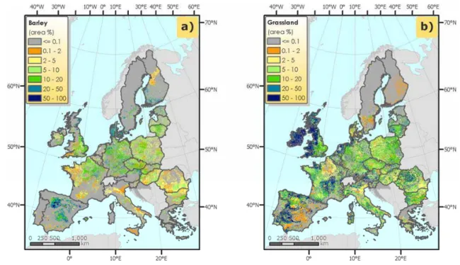
UAAR amounts to 47%, with national values ranging from 8% in Finland and Sweden to more than 70% in United King-dom and Ireland. There are differences between the “old” Member States (EU15), members of the European Union be-fore 1 May 2004 and the “new” Member States that became member of the EU at or after this date (EU12). For EU15, 75% of the area belongs to a spatial unit with some agricul-tural use, a quarter of which has a UAAR less than or equal to 5%. Higher average shares of UAAR are found for EU12 countries, where most of the surface is covered by HSMUs with some agricultural use (89%) with only one-tenth hav-ing 5% or less of agricultural land use. Specific examples of agricultural land use maps obtained are shown in Fig. 4 for barley and permanent grassland for the year 2000.
The livestock density maps highlight the huge variability in stocking densities found in Europe as a result of differ-ences in farming systems and natural conditions. The high-est stocking densities are found in parts of Netherlands, gium, some German counties close to Netherlands and
Bel-gium, Bretagne and the Po Plain in Italy. In such cases, mixed farming systems are found both featuring ruminants and non-ruminants, and with fattening processes based on concentrates. The lowest stocking densities are linked to regions where specialized crop farms are the main produc-tion system, often found where, over time, large-scale arable farming under favourable conditions has developed.
3.3 Results input data
3.3.1 Nitrogen application
On average 106 kg N of mineral fertilizer and 61 kg N con-tained in manure are applied per hectare to agricultural land in Europe. Hence the share of manure nitrogen in the to-tal nitrogen application is 37%, which is similar to the 33% share reported in the national GHG inventory of the
Eu-ropean Communities (EEA, 2006). Obviously, there are
large differences between different countries, according to the intensity of livestock production, as well as among crops. Table 3 shows the average national nitrogen application rates for mineral fertilizer and manure by crop. Belgium, Den-mark and Netherlands are able to cover most of their nitrogen
Fig. 4. Examples for the land use map: (a) barley, (b) permanent grassland. needs by using manure; France, Portugal and United King-dom must purchase most of the applied nitrogen from min-eral sources.
The low average manure application rates in countries like France, Portugal and United Kingdom can be explained by several factors. First, compared to Belgium, Denmark and Netherlands, the average livestock densities are considerable lower. Second, stocking densities are dominated by rumi-nants which are linked to grassland. And third, the main arable cropping regions are dominated by specialized farms without animals, especially in France and United Kingdom.
3.3.2 Export of nitrogen with harvested material
Plants nitrogen uptake is the largest single pathway of ni-trogen added or recycled during a year. With an average of
233 kg N ha−1 y−1 for all countries and crops simulated, it
balances approximately the total input of nitrogen by min-eral fertilizer and manure application, nitrogen fixation and
nitrogen deposition (217 kg N ha−1y−1; see Table 4). The
ratio of nitrogen uptake to nitrogen delivery is highest for ce-reals such as rye and barley where twice as much nitrogen is contained in the plant than was added to the system. Sun-flower and paddy rice, on the other hand, took up only half of the applied nitrogen. Obviously a large part of the nitrogen that accumulates in the biomass will remain in the system as only a – crop-dependent – fraction is removed at harvest. Furthermore, recycling of nitrogen in the soil (mineralization of organic matter and crop residues) contributes differently to the pool of available nitrogen.
For all crops considered, the amount of nitrogen in the har-vested material was from 40% to 70% of the total plant
nitro-gen. For the above-ground biomass which is not harvested, it was assumed that 90% of the crop residues was left on the field (Li et al., 1994). These figures suggest a simulated ni-trogen surplus between 15% for oats and more than 80% for sunflower. Nitrogen surplus pathways will be discussed in more detail in Sect. 3.4.
As described above, nitrogen application rates were cal-culated as a function of the estimated (above-ground) nitro-gen uptake. This information was translated into potential to-tal plant carbon to be achieved without environmento-tal stress. Generally the reduction in assimilated plant carbon from the optimal situation was relatively stable for the different crops. Looking at all simulations, plant biomass was only 66% of the potential value. Most cereals (soft wheat, durum wheat, rye and barley) had approximately 70%–80% of the optimal yield, with maize and durum wheat scoring lowest. These crops achieved only half of the potential biomass, similar to potatoes and sugar beet. Paddy rice and soya were closest to their potential biomass carbon (approximately 90%). In most cases the model was able to achieve the pre-defined distribution of carbon over the plant components (root, shoot and grain), which shows that the phenology provided to the model (sowing and harvest dates) corresponds to the param-eterization of plant development. Problems were observed only for crops growing in Finland, where plant maturation was simulated too slowly, resulting in larger fractions of car-bon allocated in root and shoot.
3.3.3 Topsoil organic carbon content
We simulated a loss of SOC of 25% or 23 t C ha−1
Table 3. Application of mineral fertilizer and manure nitrogen [kg N ha−1].
N-input∗ SWHE DWHE RYEM BARL OATS MAIZ PARI RAPE SUNF SOYA PULS POTA SUGB TOMA OVEG OFAR Average
Austria (a) 73 75 36 69 48 83 68 83 144 59 65 137 210 76 19 75 (b) 6 24 12 25 17 101 33 20 27 48 12 30 16 5 53 38 Belgium$ (a) 230 82 24 99 12 154 7 39 164 500 15 288 58 (b) 11 31 64 43 411 80 118 346 171 73 105 49 318 Denmark (a) 113 38 53 9 46 121 186 340 36 79 (b) 161 61 123 112 57 344 299 304 225 177 Finland (a) 125 46 83 82 65 35 26 53 62 432 59 29 81 (b) 45 3 24 43 20 47 48 56 16 9 1 61 33 France (a) 192 115 80 140 79 138 96 101 190 2 100 130 163 40 79 156 (b) 9 15 10 10 19 61 37 39 48 18 95 86 139 14 37 28 Germany (a) 274 176 169 92 114 44 152 129 44 95 161 279 47 154 183 (b) 14 13 20 6 10 175 65 97 32 107 113 65 30 79 54 Greece (a) 63 47 147 47 18 146 145 23 236 90 110 129 56 44 56 (b) 9 17 34 1 5 1 1 9 14 1 10 1 1 8 15 Ireland (a) 210 210 191 75 54 223 44 121 131 (b) 23 15 2 2 78 67 Italy (a) 134 67 87 145 95 132 184 54 136 269 21 171 104 188 45 34 94 (b) 1 3 4 2 7 163 157 27 61 49 4 119 79 49 60 48 66 Netherlands (a) 186 41 66 163 50 79 78 207 466 343 75 343 119 (b) 173 56 301 163 116 178 15 272 123 216 214 Portugal (a) 34 29 32 34 16 112 118 9 66 6 64 97 (b) 1 0 26 20 35 27 18 Spain (a) 65 40 100 59 59 227 147 59 31 111 5 44 125 186 69 73 60 (b) 7 0 26 10 7 54 136 46 34 31 59 62 27 20 169 26 14 Sweden (a) 182 67 98 70 56 81 399 90 47 63 (b) 76 5 39 41 52 5 4 1 80 65 United (a) 123 197 72 91 71 59 115 65 72 107 24 307 31 60 104 Kingdom (b) 23 11 7 11 25 40 20 95 47 65 13 22 23 26 20 Average (a) 171 61 152 64 92 113 177 131 51 173 18 126 119 205 54 55 106 (b) 48 5 19 22 27 138 157 52 36 37 26 143 65 53 61 108 61
∗(a) Mineral fertilizer nitrogen; (b) Manure nitrogen; $: Luxembourg included in the numbers of Belgium; SHWE: soft wheat, DWHE:
durum wheat, OCER: other cereals, BARL: barley, RYEM: rye, OATS: oats, MAIZ: maize; PARI: paddy rice, SUNF: sun flower, SOYA: soya, POTA: potatoes, SUGB: sugar beet, ROOF: root fodder crops, TOMA: tomatoes, OVEG, other vegetables, OFAR: fodder on arable land. -20% 0% 20% 40% 60% 80% 100% 120% 0 10 20 30 40 50 60 70 80 90 100 Running simulation year after initialization
Relative decrease of soil organic carbon stocks Relative decrease of N2O fluxes
Fig. 5. Soil organic carbon content in the top 30 cm of soils (dotted symbols) and N2O flux from the soil surface (dashed symbols), both relative to the situation in the initial simulation year.
and management data. Losses of organic carbon through mineralization processes were very high in the first simu-lation years with an average loss of 0.5 t C ha−1y−1during the first decade slowing down to 0.1 t C ha−1y−1during the last decade. The latter value is close to estimates of cur-rent carbon losses from European croplands (Vleeshouwers and Verhagen, 2002; see also Smith et al., 2005a).
Fig-0 50 100 150 200 250 300 350 400 ]0 … 0 .2 ] ]0 .2 … 0 .4 ] ]0 .4 … 0 .6 ] ]0 .6 … 0 .8 ] ]0 .8 … 1 ] ]1 … 1 .2 ] ]1 .2 … 1 .4 ] ]1 .4 … 1 .6 ] ]1 .6 … 1 .8 ] ]1 .8 … 2 ] ]2 …
SWHE BARL MAIZ POTA SUGB OFAR
F re q u e n c y ( n u m b e r o f s im u la ti o n s )
Soil organic carbon content in the top 30 cm after the end fo the simulation period relative to the initialization conditions
Fig. 6. Histogram for relative changes in soil organic carbon in the top 30 cm of soil for selected crops. SWHE: soft wheat; BARL: barley; MAIZ: maize; POTA: potatoes; SUGB: sugar beet; OFAR: fodder on arable land.
ure 5 (dotted symbols) shows that after a 98 years simulation, the average soil organic carbon stocks in the top 30 cm over
all spatial simulation units dropped from 93±45 t C ha−1to
70±30 t C ha−1. Only 15% of the simulations showed an
in-crease of SOC. The distribution of relative changes for se-lected crops is slightly skewed (Fig. 6). Significant increases
in SOC (>50% of the initial value) occurred only for maize. The majority of simulation units stayed within 20% of the initial carbon content.
The dashed symbols in Fig. 5 show the impact of declin-ing SOM content on simulated N2O fluxes relative to the
ini-tial situation over all simulated spaini-tial modelling units. The
average N2O flux declines faster than the average relative
N2O flux in the single spatial modelling units. While initial
N2O fluxes were 17 kg N–N2O ha−1y−1, they were reduced
after the 98 year simulation to 2.8 kg N–N2O ha−1y−1. This
suggests that some un-realistically high topsoil organic
car-bon estimates led to extremely high N2O fluxes in the first
years of the spin-up simulation but declined quickly there-after, diminishing their weight in the mean N2O flux. Spatial
variability is very high throughout the years, though it creases with time. The standard deviation of the average de-crease of the relative N2O flux is 200% in the tenth year,
re-flecting large reductions in a few modelling units and smaller
reductions in many more modelling units. N2O fluxes and the
standard deviation of mean N2O fluxes are relatively stable
after 50 simulation years.
3.4 Simulation results
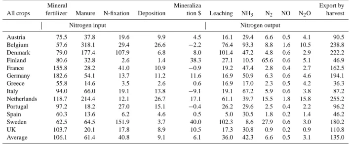
All of the results presented in this section are related to the first simulation year after the 98 years spin-up run. Since this is a methodological paper, we restrict the presentation of the simulated nitrogen budget to the national scale. Table 4 shows a summary of the quantified, i.e. reported elements in the N budget aggregated to the country scale. Outputs of nitrogen by nitrogen losses and export by plant material ei-ther through plant products or crop residues are compared to nitrogen inputs via nitrogen application, deposition, fix-ation and release of nitrogen through net mineralizfix-ation of SOM. Net mineralization of organic matter leads in some countries to a loss of nitrogen if SOM has been simulated to build up in that country. The two sides of the balance are large fluxes of nitrogen and span a large range from
77 kg N ha−1y−1(Greece) to 430 kg N ha−1y−1(Belgium).
The export of nitrogen with the crop has been calculated as the residual from the difference between nitrogen inputs and outputs to close the nitrogen budget at the soil surface. Errors may occur, due to unaccounted sources or sinks of nitrogen in the simulations, such as allocation of biologically fixed ni-trogen in soil compartments or leaching of organic matter. However, these discrepancies are considered to be minimal, as was found in simulations where crop development was suppressed. Here the nitrogen was essentially balanced. Ad-ditionally, C/N ratios of the exported plant biomass were in most cases identical to or slightly higher than the pre-defined C/N ratios in grain (due to the higher C/N ratio in plant shoot biomass). Therefore, the error introduced by using a con-stant C/N ratio for mineralized soil organic matter is likely to be small. DNDC simulates different pools of organic
mat-ter with defined C/N ratios. The C/N ratio of litmat-ter varies from very labile (C/N=5) through labile (C/N=50) to resis-tant litter (C/N=200). Other compartments comprise micro-bial biomass, humads and humus, which are all characterized by a C/N ratio of 12.
Nitrogen surplus is generally an important indicator of the environmental impact of agriculture on one hand, and of the effectiveness of environmental policies on the other hand. Calculating the nitrogen surplus as the ratio of nitrogen not taken up by plants (both in harvested material and in removed crop residues) to the total nitrogen input during the simula-tion year, gave results ranging between 26% (United King-dom) and 55% (Italy). The regional average nitrogen surplus was 38%.
4 Discussion
4.1 Spatial simulation units
Regional or (sub)continental modelling studies often run their model on a regular grid of varying size depending on the area covered by the format of available data sets and the scope of the simulations. Roelandt et al. (2006) for example
worked on predicting future N2O emissions from Belgium
relying on climate scenarios that were available for a 10’ lon-gitude and latitude grid, while Kesik et al. (2005) linked the simulation of nitrogen oxides emissions from European for-est soils to the available climate data set and ran the model on a 50 km×50 km raster. Vuichard et al. (2007) estimated the GHG balance of European grasslands but due to com-puting limitations they restricted the simulations to a 1◦×1◦
grid. These approaches are efficient for fast responses to pos-sible developments or for delivering a first estimate of large-scale emissions. For detailed analysis, however, they lack the link to realistic land use data (Roelandt et al., 2006) and are too coarse for capturing local heterogeneities (Vuichard et al., 2007). For a better representation of land use, many authors run their models within the administrative bound-aries for which regional statistics are available. Examples of this approach include simulation studies on about 2 500 Chi-nese counties to estimate soil organic carbon storage (Tang et al., 2006) or GHG emissions from rice cultivation (Li et al., 2006) using the DNDC model. To assess regional hetero-geneity, the Most Sensitive Factor method (Li et al., 2005) is used giving a reasonable range of emission values with a high probability to capture the true value. This “administrative approach” is also used if the study aims to give support to, or for comparison with, national GHG estimates performed with the IPCC emission-factor approach (e.g. Li et al., 2001; Brown et al., 2002; Del Grosso et al., 2005; Mulligan, 2006). Mulligan points out, however, that most of the uncertainty in the emission estimates stem from the large range of envi-ronmental conditions encountered within a single modelling unit.
Table 4. Summary of the quantified nitrogen budget, aggregated to country-scale. All values are given in kg N ha−1.
Mineral Mineraliza Export by
All crops fertilizer Manure N-fixation Deposition tion $ Leaching NH3 N2 NO N2O harvest
Nitrogen input Nitrogen output
Austria 75.5 37.8 19.6 9.9 4.5 16.1 29.4 6.6 0.5 4.1 90.5 Belgium 57.6 318.1 29.4 26.6 −2.2 76.4 93.3 8.8 1.6 10.5 238.8 Denmark 79.0 177.4 107.9 6.8 8.0 101.4 47.2 4.8 0.6 2.9 222.2 Finland 80.6 32.8 2.6 1.4 38.3 27.1 10.5 65.6 0.6 5.1 46.9 France 155.8 28.2 41.0 10.9 −0.9 19.2 47.4 2.8 0.4 2.7 162.5 Germany 182.6 54.1 13.7 11.2 11.6 16.9 50.9 6.3 0.6 4.6 194.1 Greece 55.8 14.6 3.5 2.6 0.6 16.9 17.0 2.3 0.5 4.2 36.3 Italy 94.0 66.0 19.1 13.8 −9.1 19.1 67.2 5.9 0.6 3.8 87.2 Netherlands 118.7 214.4 12.1 26.7 17.1 61.1 39.7 15.5 1.8 15.8 255.2 Portugal 97.2 18.2 27.0 15.1 −0.4 26.2 29.6 2.5 0.4 2.2 96.2 Spain 60.3 13.6 6.2 4.6 0.5 5.0 30.5 1.8 0.2 1.4 46.2 Sweden 62.5 64.5 151.9 3.7 40.0 102.3 8.6 27.9 0.6 3.0 180.2 UK 103.7 20.1 17.8 8.9 10.5 17.3 30.8 0.9 0.2 0.9 110.8 Average 106.1 61.4 40.8 9.1 6.1 36.0 42.3 6.6 0.5 3.1 135.0
$ Net mineralization calculated from simulated changes in soil organic stocks using an average soil C/N ratio of 12.
To overcome these problems, other studies have used the geometry of the available information on soil properties to delineate the modelling units used. For large-scale applica-tion, as in the Grant et al. (2004) assessment of the impact
of agricultural management on N2O and CO2emissions in
Canada, representative soil type and soil texture combina-tions were defined covering the seven major soil regions in Canada. Changes in soil organic carbon stocks or fluxes of GHGs were estimated on the basis of landscape units generated by an intersection of a land-use map and a soil map for Belgium (Lettens et al., 2005) or a region in Ger-many (Bareth et al., 2001). An additional intersection with a
climate map was done in a study on N2O emissions from
agriculture in Scotland (Lilly et al., 2003). So far, how-ever, these very detailed analyses were restricted to relatively small countries or regions due to limitations of computing re-sources.
Schmid et al. (2006) describe a very detailed approach to simulate soil processes in Europe with the biophysical model EPIC. By intersecting landscape variables that are considered stable over time (elevation, slope, soil texture, depth of soil and volume of stones in the subsoil) they obtained a layer of more than 1 000 homogeneous response units. Each of these units was divided, on average, into 10 individual simu-lation units by overlaying various maps such as climate, land cover, land use/management and administrative boundaries. Individual simulation units were then regarded as representa-tive field sites and the estimated field impact from simulated management practices was uniformly extrapolated to the en-tire unit.
Our approach has many similarities to the approach de-scribed by Schmid et al. (2006); in both cases the philosophy
is to develop a framework integrating both environmental and socio-economic impacts on soil processes. The main differ-ences, however, are the following:
– In Schmid et al. (2006), selected soil characteristics are used to delineate the homogeneous response units, while in the present study each geometrical unit of the soil database (the so-called SMU) is maintained in the delineation of the homogeneous spatial mapping units defined. Each SMU is a unique combination of one or several soil types. Preliminary land use simulations suggested that soil type is an integrative characteristic with relevance for both the agronomic-based choice of the use of the land and for the environmental response to agronomic pressures, yielding more reliable land use estimates. Unfortunately, soil types within an SMU are not geo-referenced and soil characteristics in use (tex-ture, topsoil organic carbon content, etc.) are defined at the scale of the SMU only. Integration of the pedo-transfer functions into the land use mapping model and consistent estimation of soil characteristics at the level of soil types will be one of the major improvements to the present approach in the near future.
– The time window for which our methodology is appli-cable is rather narrow and linked – through the CAPRI model – to the time horizon of agricultural projections, usually about 10 years. However, the methodology used for downscaling the regional information to the spa-tial calculation units could easily be incorporated in any other socio-economic modelling framework, pro-vided that the main driving parameters are consistently calculated (mineral fertilizer consumption and manure
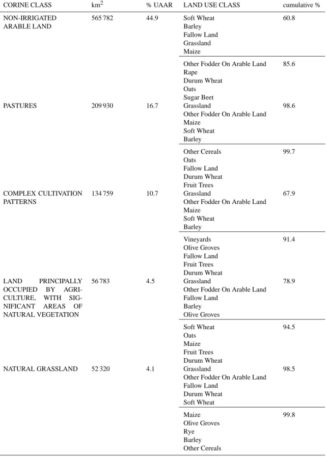
Table 5. Main statistics on the layer of the homogeneous spatial mapping units (HMSUs) for EU27 without Malta and Cyprus.
CORINE CLASS km2 % UAAR LAND USE CLASS cumulative %
NON-IRRIGATED ARABLE LAND 565 782 44.9 Soft Wheat Barley Fallow Land Grassland Maize 60.8
Other Fodder On Arable Land Rape Durum Wheat Oats Sugar Beet 85.6 PASTURES 209 930 16.7 Grassland
Other Fodder On Arable Land Maize Soft Wheat Barley 98.6 Other Cereals Oats Fallow Land Durum Wheat Fruit Trees 99.7 COMPLEX CULTIVATION PATTERNS 134 759 10.7 Grassland
Other Fodder On Arable Land Maize Soft Wheat Barley 67.9 Vineyards Olive Groves Fallow Land Fruit Trees Durum Wheat 91.4 LAND PRINCIPALLY OCCUPIED BY
AGRI-CULTURE, WITH
SIG-NIFICANT AREAS OF
NATURAL VEGETATION
56 783 4.5 Grassland
Other Fodder On Arable Land Fallow Land Barley Olive Groves 78.9 Soft Wheat Oats Maize Fruit Trees Durum Wheat 94.5
NATURAL GRASSLAND 52 320 4.1 Grassland
Other Fodder On Arable Land Fallow Land Durum Wheat Soft Wheat 98.5 Maize Olive Groves Rye Barley Other Cereals 99.8
Table 6. Application rates of mineral fertilizer nitrogen for selected crops/countries [kg N ha−1] (Source: FAO/IFA/IFDC/IPI/PPI, 2002).
Wheat Barley Maize Rape Pulses Potatoes Sugar b. Veget. Fodder Total
Austria 82 70 184 80 30 110 90 110 8 75 Belgium 115 98 108 2 110 85 108 92 33 Denmark 155 100 150 20 155 110 110 62 116 Finland 120 78 110 83 100 100 85 41 France 85 72 80 40 70 120 80 47 Germany 165 150 150 170 25 140 145 165 94 131 Greece 150 78 100 120 100 140 118 18 Ireland 80 120 170 155 150 35 145 45 52 59 Italy 70 75 190 40 200 140 170 64 Netherlands 160 110 150 120 180 120 49 Portugal 190 85 44 180 20 168 108 125 30 38 Spain 95 90 225 109 9 142 178 205 27 75 Sweden 80 60 160 100 5 100 150 120 80 73 United Kingdom 183 118 185 5 155 100 125 75 30 EU15 92 91 101 158 14 129 136 109 54 69
nitrogen excretion, acreages for the cultivation of the crops, and their respective productivity).
– While the individual simulation units allow for consis-tent integration of biophysical impact vectors in eco-nomic land use optimization models, the HSMUs are an integral part of both the economic and the biophysical model. This allows us to intimately link both modelling approaches, which is a prerequisite for efficient environ-mental policy impact assessment.
4.2 Land use map
The legend of the CORINE Land Cover map contains eleven pure or mixed agricultural classes. Interpretation, particu-larly of the mixed classes such as “complex cultivation pat-terns”, is very different for different regions in Europe. The typical land-use mix for this class differs largely between countries. Complex cultivation patterns, according to the definition (Bossard et al., 2000), consist of a “juxtaposition of small parcels of diverse annual crops, pasture and/or per-manent crops” with built-up parcels covering less than 30%. In Spain, for example, permanent crops and cereals account for 35% and 15% of the area covered by this class, respec-tively, while in Germany cereals have a large share (40%) and permanent crops are insignificant. In addition, comparisons of CORINE with detailed statistics resulted in large disagree-ments (Schmit et al., 2006). At the European scale a simple downscaling procedure on the basis of CORINE would there-fore lead to biased estimation of land use shares.
Hence, from a conceptual point of view, the procedure de-scribed in Sect. 2.3 can be interpreted as a “calibration” of the CORINE Land Cover/Use map, giving more detailed in-formation on the share of individual crops in mixed and
het-erogeneous classes (e.g. non-irrigated arable land and com-plex cultivation pattern, respectively), but also on the share of non-agricultural area for each class. An overview of crop associations in the main CORINE land cover classes cover-ing about 80% of the UAAR in EU15 is given in Table 5. Grassland covers 14% of the surface area of Europe and is the most important agricultural land use for most countries with shares of up to 75% of the UAAR (Ireland).
We compared the results of our methodology by dis-aggregating NUTS 2 data from the agricultural census of the European Union, the FSS (FSS2000, European Com-mission, 2003b) and calculating the share of mis-classified agricultural area for regions where data were available at a more detailed level (NUTS 3). The validation procedure is described in detail in the appendix. We obtained an area weighted mean error of ∼12.2% for Europe. Compared with a “no-disaggregation” scenario, we achieved a reduction of the error by a factor of two.
With the exception of non-irrigated arable land, grassland occupies the largest share of the area of the mixed land cover classes. The correspondence is highest (92%) for the class “natural grassland”. For other pure land cover classes, our model predicts high correspondence with CORINE, i.e. 78% for rice fields and 81% for olive grows. This makes it even more astonishing that in regions with a high percentage of misclassified area, grassland often accounts for a significant part of the errors. This suggests that misclassification errors might not only be a consequence of a poor dis-aggregation procedure but also a result of inconsistent data sources. Gen-erally grassland area tends to be larger in the FSS statistics than in the CORINE land cover map (Grizzetti et al., 2007). For example, the CORINE land cover map reports about 2 Mha “Pasture” and “Natural Grassland” in Spain while the
FSS reports about 9 Mha of Grassland. Nonetheless the dis-aggregation is a significant improvement compared to the as-sumption of identical cropping patterns within each NUTS 2 region. A detailed analysis for Belgium (Schmit et al., 2006) found low reliability for grassland in CORINE as less than half of the pixels that are classified as grassland in CORINE corresponded to grassland pixels in the reference map. Even worse, only a little more than 10% of the grassland in the reference map was correctly represented by CORINE.
Very rarely, single crops are considered in a model exer-cise or in other applications. Usually the crops are grouped according to their physical similarity or their analogous agri-cultural practices. If we consider only crop groups (cereals, fallow land, rice and oilseeds, industrial crops, permanent crops and grassland and fodder), some of the distribution er-rors level out as, within these groups, the site condition re-quirements of the plants are sometimes very similar and can-not be easily distinguished by the model. For countries in-cluded in the calculation, the dis-aggregation error decreases from 12% for individual crops to 8% for crop groups. The error for very coarse crop classes (arable crops, permanent crops and grassland and fodder) is still lower (6.2%), and 3.4% of the total UAAR was attributed to the wrong NUTS 3 regions.
4.3 Input data
4.3.1 Fertilizer/manure input
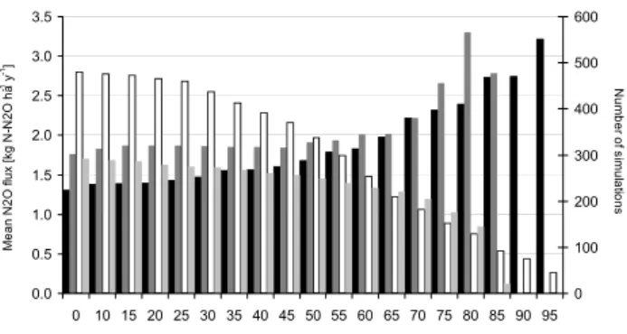
In the majority of the cases, the nitrogen application rates from CAPRI yielded plausible results when compared to crop removals, especially in the case of mineral applica-tion rates where at least average naapplica-tional rates for cer-tain crops or crop groups could be used in the estima-tion process. If we compare the mineral applicaestima-tion rates for individual crops and countries with the information ob-tained from the International Fertilizer Industry Association (FAO/IFA/IFDC/IPI/PPI, 2002) we find considerable differ-ences (Table 6). The reason can be found in our methodol-ogy that links total nitrogen application to nitrogen uptake by plants. This in turn is available from statistical sources. Our approach tries to minimize both the deviation from the IFA-application rates of mineral fertilizer nitrogen and the share of nitrogen obtained from manure, taking into consideration the availability of manure nitrogen in the region. The IFA estimates are the result of a negotiation procedure between different institutions and are based on information obtained from questionnaires to national administration and industry representatives (FAO/IFA/IFDC/IPI/PPI, 2002). As they ig-nore the regional effect of the distribution of the animals, small deviations from the IFA estimates might occur. These deviations depend on the location of the cropland in relation to the stocking density of animals and the soil quality in the region. 0.0 0.5 1.0 1.5 2.0 2.5 3.0 3.5 0 10 15 20 25 30 35 40 45 50 55 60 65 70 75 80 85 90 95 Percentage of estimated simulated carbon export during harvest [%]
0 100 200 300 400 500 600
Mean N2O flux - Soft wheat Mean N2O fluxes - Barley Number of simulations - Soft wheat Number of simulations - Barley
M e a n N 2 O f lu x [k g N -N 2 O h a -1 y -1] N u m b e r o f si m u la tio n s
Fig. 7. Number of simulations yielding at least a given percentage of estimated plant carbon uptake for soft wheat and barley (light-coloured columns, right axis), and mean N2O fluxes estimated on the respective sub-samples (dark coloured columns, left axis).
4.3.2 Yield
Our approach aims to match as far as possible the uptake of carbon and nitrogen simulated with the biophysical model DNDC with the available yield statistics at the regional level and the estimated information (yield downscaled to the spa-tial calculation unit). Differences are due to stress situations that tend to reduce plant growth in the simulation model. As an example, Fig. 7 shows the number of simulations and the
corresponding mean N2O fluxes, if only simulations
yield-ing a minimum of the carbon export estimated with CAPRI are taken into account. The figure compares two cereals, soft wheat and barley, which differ with respect to simulated
car-bon export and N2O fluxes. Soft wheat has stricter
require-ments on environmental conditions than barley. Due to its lower capability to store humidity, it has a higher demand on summer precipitation. Therefore, stress is much higher for soft wheat with a lower average relative yield. While the me-dian N2O flux of all simulations with soft wheat cultivation
is only 1.3 kg N–N2O ha−1y−1, it increases continuously if
plant uptake of nitrogen gets closer to the optimum. For the last 50 simulations (approximately 7%) where at least 95%
of nitrogen export was simulated, we obtain an N2O flux
of 3.2 kg N–N2O ha−1y−1. This is similar to the emissions
from barley for non-limited simulations, while the overall median for barley with 1.8 kg N–N2O ha−1y−1is higher than
that of soft wheat.
Thus, we observe that (i) environmental conditions play a major role both in the choices of the farmers and what they are going to cultivate; in DNDC, penalties for stress condi-tions are smaller than in CAPRI and decreases in expected yield are thus strongly limited by fertilizer input; (ii) highest emissions occur on high-productivity sites, expressed rela-tive to the cultivated area or production unit.
4.3.3 Soil map
The effort invested into the development of an agricultural land use map of high resolution is justified by the need to spa-tially match agricultural activities with environmental condi-tions, mainly soil properties, which have been identified to be the major reason for high uncertainty. These efforts are cur-rently not adequately matched by the quality of the soil map. A reason for concern arises in particular from two charac-teristics of the data used, i.e. (i) soil types are not directly mapped, and (ii) the derivation of soil properties in the raster maps is done using fixed land use information.
The spatial components of the soil database of Europe, the so-called SMUs corresponding to a soil type association, comprise a varying number of soil types with unknown spa-tial location and a defined share of the SMU area. However, variations in soil organic carbon or other attributes within an SMU are accounted for by including information on land use (CORINE Land Cover 1990 map), climate and Soil Typo-logical Unit (STU). Inconsistencies might arise, particularly if the land use estimated in the present study differs largely from the land use that was used in the derivation of the soil characteristics. We tried to account for this by “filtering” out HSMUs with a high share of forest area in CORINE 1990 (European Topic Centre on Terrestrial Environment, 2000) as compared to the land use shares estimated in our approach. Nevertheless, we observed a very high average soil organic
carbon content in Finland, where only 2 764 km2 of
agri-cultural area is estimated to be cultivated on organic soils (Statistics Finland, 2005) corresponding to approximately 22% of the agricultural area in our database. This could re-sult in uncertainties. Based on the decomposition and deni-trification processes built in DNDC, cultivated organic soils
under humid climate conditions can have high rates of N2O
as well as dinitrogen (N2)emissions. Therefore, any
overes-timation on the combination of agricultural area with organic
soil could overestimate N2 losses and N2O emissions. We
estimate significant agricultural activities on highly organic soils (>100 t C ha−1)in Finland (barley and oats), Sweden (barley and fodder production), Belgium (maize) and Nether-lands (maize and softwheat), so that the simulated denitrifi-cation losses (see Table 4) have a higher uncertainty for those countries.
In the present study we obtained realistic soil initialization by conducting a 98 year spin-up run. Nevertheless it will be of highest priority to incorporate the estimation of soil char-acteristics into the land use share model to refine the available soil information.
4.4 General discussion
It is frequently recognized that the impact of society on the environment is costly and needs to be considered when pol-icy impact analyses are performed. Supporting tools are re-quired to answer two primary questions: “what is the impact
of a certain policy pathway?” and “how much does it cost to reduce this impact?” Prominent integrated modelling frame-works include the Integrated Model to Assess the Global En-vironment (IMAGE, Bouwman et al., 2006) and the RAINS model (e.g. H¨oglund-Isaksson et al., 2006). Integrated mod-elling systems link socio-economic analyses with environ-mental assessment, usually working with a multi-sectoral ap-proach. Due to the large number of variables they have to deal with, they are based on simple relationships or empirical functions. On the other hand, sectoral “integrated models” are able to simulate both socio-economy and environment of a single sector with great detail and are thus able to deliver targeted policy impact assessments.
For example Schneider et al. (2007) present an analysis of mitigation options in USA agriculture and forestry, with a biophysical model predicting GHG emission coefficients and carbon stock changes for various management options.
Another example of such a sectoral integrated mod-elling framework is the EFEM-DNDC system described by Neufeldt et al. (2006). In their system, the economic farm emission model EFEM is linked to the biophysical model DNDC via crop acreage and fertilizer intensity esti-mates for one of eight different regional groups in Baden-W¨urttemberg, Germany, which are composed of several mu-nicipalities with similar environmental conditions and typical production systems. The downscaling of this information to the modelling units was done on the basis of the CORINE land cover map, including a correction factor to account for differences in agricultural area between the statistics and CORINE. Our approach is very similar to the EFEM-DNDC approach. The main differences are (i) a more “elaborate” approach for downscaling, and (ii) a closer link between both modelling systems, as nitrogen application rates are adapted to the individual conditions of the spatial calculation units.
We regard both features as an essential element for an agri-cultural integrated modelling framework, particularly for a large-scale application as in the present study. One of the most important features of an integrated modelling frame-work is a consistent flow of nutrients in the various modules. The approach described above is designed to reach maximum consistency both in term of scale (scale-consistent downscal-ing from national and regional statistics to a grid based on 1 km×1 km pixels) and in terms of mass-flow through agri-cultural sub-systems.
5 Conclusions
We presented an approach that links an economic model for agriculture with a process-based simulation model for arable
soils for Europe. The procedure developed involves two
steps. The first step consists in the generation of spatially explicit information at the level of clustered 1-km grid cells on land use, animal density, and agricultural input parame-ter in the framework of the economic model CAPRI. In the


![Table 3. Application of mineral fertilizer and manure nitrogen [kg N ha − 1 ].](https://thumb-eu.123doks.com/thumbv2/123doknet/14777094.594396/11.892.76.826.134.506/table-application-mineral-fertilizer-manure-nitrogen-kg-n.webp)
![Table 6. Application rates of mineral fertilizer nitrogen for selected crops/countries [kg N ha − 1 ] (Source: FAO/IFA/IFDC/IPI/PPI, 2002).](https://thumb-eu.123doks.com/thumbv2/123doknet/14777094.594396/15.892.123.770.135.425/table-application-mineral-fertilizer-nitrogen-selected-countries-source.webp)