HAL Id: tel-02366973
https://tel.archives-ouvertes.fr/tel-02366973v2
Submitted on 29 Nov 2019
HAL is a multi-disciplinary open access archive for the deposit and dissemination of sci-entific research documents, whether they are pub-lished or not. The documents may come from teaching and research institutions in France or abroad, or from public or private research centers.
L’archive ouverte pluridisciplinaire HAL, est destinée au dépôt et à la diffusion de documents scientifiques de niveau recherche, publiés ou non, émanant des établissements d’enseignement et de recherche français ou étrangers, des laboratoires publics ou privés.
Modeling techniques for building design considering
soil-structure interaction
Reine Fares
To cite this version:
Reine Fares. Modeling techniques for building design considering soil-structure interaction. Structures. Université Côte d’Azur, 2018. English. �NNT : 2018AZUR4103�. �tel-02366973v2�
1
Techniques de modélisation pour la conception des
bâtiments parasismiques en tenant compte de
l’interaction sol-structure
Modeling techniques for building design considering
soil-structure interaction
Reine FARES
Laboratoire Géoazur – Laboratoire Jean Alexandre Dieudonné
Présentée en vue de l’obtention du grade de docteur en sciences pour l’ingénieur de
l’Université Côte d’Azur
Dirigée par : Anne Deschamps
Co-encadrée par : Maria Paola Santisi d’Avila Soutenue le : 16/11/2018
Devant le jury, composé de :
Pierfrancesco Cacciola Jean-François Semblat Etienne Bertrand Luca Lenti Principal lecturer Professeur Directeur de recherche Chargé de recherche University of Brighton ENSTA ParisTech CEREMA Méditerranée IFSTTAR Champs-sur-Marne
THÈSE DE DOCTORAT
3
Techniques de modélisation pour la conception des bâtiments parasismiques en tenant compte de l’interaction sol-structure
Résumé
La conception des bâtiments selon le code sismique européen ne prend pas en compte les effets de l'interaction sol-structure (ISS). L'objectif de cette recherche est de proposer une technique de modélisation pour prendre en compte l’ISS et l'interaction structure-sol-structure (ISSS).
L'approche de propagation unidirectionnelle d’une onde à trois composantes (1D-3C) est adoptée pour résoudre la réponse dynamique du sol. La technique de modélisation de propagation unidirectionnelle d'une onde à trois composantes est étendue pour des analyses d'ISS et ISSS. Un sol tridimensionnel (3-D) est modélisé jusqu'à une profondeur fixée, où la réponse du sol est influencée par l’ISS et l’ISSS, et un modèle de sol 1-D est adopté pour les couches de sol plus profondes, jusqu'à l'interface sol-substrat. Le profil de sol en T est assemblé avec une ou plusieurs structures 3-D de type poteaux-poutres, à l’aide d’un modèle par éléments finis, pour prendre en compte, respectivement, l’ISS et l’ISSS dans la conception de bâtiments.
La technique de modélisation 1DT-3C proposée est utilisée pour étudier les effets d’ISS et analyser l'influence d'un bâtiment proche (l'analyse d’ISSS), dans la réponse sismique des structures poteaux-poutres. Une analyse paramétrique de la réponse sismique des bâtiments en béton armé est développée et discutée pour identifier les paramètres clé du phénomène d’ISS, influençant la réponse structurelle, à introduire dans la conception de bâtiments résistants aux séismes.
La variation de l'accélération maximale en haut du bâtiment avec le rapport de fréquence bâtiment / sol est tracée pour plusieurs bâtiments, chargés par un mouvement à bande étroite, excitant leur fréquence fondamentale. Dans le cas de sols et de structures à comportement linéaire, une tendance similaire est obtenue pour différents bâtiments. Cela suggère l'introduction d'un coefficient correcteur du spectre de réponse de dimensionnement pour prendre en compte l’ISS. L'analyse paramétrique est répétée en introduisant l'effet de la non-linéarité du sol et du béton armé.
La réponse sismique d'un bâtiment en béton armé est estimée en tenant compte de l'effet d'un bâtiment voisin, pour un sol et des structures à comportement linéaire, dans les deux cas de charge sismique à bande étroite excitant la fréquence fondamentale du bâtiment cible et du bâtiment voisin. Cette approche permet une analyse efficace de l'interaction structure-sol-structure pour la pratique de l'ingénierie afin d'inspirer la conception d'outils pour la réduction du risque sismique et l'organisation urbaine.
Mots clés : Interaction Structure-Sol-Structure ; interaction Sol-Structure ; méthode d’éléments finis ; propagation d’onde ; chargement sismique à trois composantes ; béton armé ; comportement non-linéaire.
5
Modeling techniques for building design considering soil-structure interaction
Abstract
Building design according to European seismic code does not consider the effects of soil-structure interaction (SSI). The objective of this research is to propose a modeling technique for SSI and Structure-Soil-Structure Interaction (SSSI) analysis.
The one-directional three-component (1D-3C) wave propagation approach is adopted to solve the dynamic soil response. The one-directional three-component wave propagation model is extended for SSI and SSSI analysis. A three-dimensional (3-D) soil is modeled until a fixed depth, where the soil response is influenced by SSI and SSSI, and a 1-D soil model is adopted for deeper soil layers until the soil-bedrock interface. The T-soil profile is assembled with one or more 3-D frame structures, in a finite element scheme, to consider, respectively, SSI and SSSI in building design.
The proposed 1DT-3C modeling technique is used to investigate SSI effects and to analyze the influence of a nearby building (SSSI analysis), in the seismic response of frame structures.
A parametric analysis of the seismic response of reinforced concrete (RC) buildings is developed and discussed to identify the key parameters of SSI phenomenon, influencing the structural response, to be introduced in earthquake resistant building design.
The variation of peak acceleration at the building top with the building to soil frequency ratio is plotted for several buildings, loaded by a narrow-band motion exciting their fundamental frequency. In the case of linear behaving soil and structure, a similar trend is obtained for different buildings. This suggests the introduction of a corrective coefficient of the design response spectrum to take into account SSI. The parametric analysis is repeated introducing the effect of nonlinear behaving soil and RC.
The seismic response of a RC building is estimated taking into account the effect of a nearby building, for linear behaving soil and structures, in both cases of narrow-band seismic loading exciting the fundamental frequency of the target and nearby building. This approach allows an easy analysis of structure-soil-structure interaction for engineering practice to inspire the design of seismic risk mitigation tools and urban organization.
Keywords: Structure-Soil-Structure Interaction; Soil-Structure interaction; finite element method; wave propagation; three-component seismic motion; reinforced concrete; nonlinear behavior.
7 Résumé ... 3 Abstract ... 5 Table of Contents ... 7 List of Acronyms ... 11 List of Figures ... 13 List of Tables ... 21 Acknowledgements ... 23 Introduction ... 27
Chapter 1 - Overview on soil and structural dynamics ... 39
1.1 Introduction to structural dynamic problem ... 40
1.1.1. Single degree of freedom (SDOF) ... 40
1.1.2. Numerical solution of the dynamic equilibrium equation for SDOF oscillators 42 1.1.3. Dynamic study of a MDOF system in the frequency domain ... 42
1.1.4. Dynamic equilibrium for MDOF structures ... 44
1.2 Numerical methods ... 46
1.2.1 Finite difference method ... 46
1.2.2 Finite element method... 47
1.2.3 Spectral element method ... 48
1.2.4 Boundary element method ... 48
1.3 Site effect ... 49
1.3.1. Impact of soil characterization ... 49
1.3.2. Impact of the soil constitutive model ... 51
1.4 Soil structure interaction ... 52
1.4.1. Observations on existing building and prototype experiments ... 53
1.4.2. Analytical study ... 54
1.4.3. Numerical study ... 55
1.5 Structure-soil-structure interaction ... 58
1.5.1. Analytical study ... 58
8
1.5.3. Numerical study ... 60
1.6 Conclusion ... 62
Chapter 2 - One-dimensional three-component wave propagation model for soil-structure interaction ... 63
2.1. 1D-3C wave propagation model ... 64
2.1.1. Spatial discretization of soil domain and boundary conditions ... 64
2.1.2. Soil constitutive relationship: Iwan’s model... 67
2.1.3. Elasto-plastic model in Abaqus ... 69
2.1.4. Building model... 72
2.1.5. Time discretization... 73
2.1.6. Soil domain area concerned by the SSI ... 73
2.2. Input data ... 74
2.2.1. Soil data ... 74
2.2.1. Building data ... 75
2.2.2. Input motion ... 76
2.2.3. Signal processing of the output motion ... 78
2.3. Verification of the proposed model ... 78
2.3.1. Comparison with other codes... 79
2.4. 1D-3C vs 3D-3C wave propagation model for vertical propagation ... 82
2.5. SSI analysis ... 86
2.6. Conclusion ... 89
Chapter 3 - One-directional three-component wave propagation in a T-shaped soil domain for SSI and SSSI ... 91
3.1. 1DT-3C wave propagation model for SSI and SSSI analyses ... 92
3.2. Verification of the proposed model ... 94
3.2.1. Input data ... 94
3.2.1. Verification ... 95
3.3. SSI analysis ... 98
3.3.1. Impact of the excitation frequency on the structural response ... 98
3.3.2. SSI estimation ... 99
3.3.3. 1st vs 2nd natural frequency ... 100
3.4. Conclusion ... 102
Chapter 4 - Response spectrum for structural design considering soil-structure interaction 105 4.1. 1DT-3C wave propagation model ... 106
9
4.2. Input data for the parametric analysis ... 108
4.2.1. Soil profiles ... 108
4.2.2. RC buildings ... 109
4.2.3. Input motion ... 111
4.3. SSI analysis ... 111
4.3.1. Linear elastic analyses ... 112
4.3.2. Effect on SSI of soil and structure nonlinear behavior ... 115
4.4. Conclusion ... 120
Chapter 5 - Structure-soil-structure interaction analysis ... 123
5.1. 1DT-3C wave propagation model for SSSI analysis ... 124
5.2. Input data for the parametric analysis ... 124
5.2.1. Soil profiles ... 124
5.2.2. Buildings characteristics ... 125
5.2.3. Input motion ... 126
5.3. SSSI analysis ... 126
5.3.1. SSSI versus SSI... 126
5.3.2. SSSI parametric analysis... 131
5.4. Semi-infinite elements and dashpot boundary conditions ... 134
5.4.1. Semi-infinite elements vs dashpots ... 137
5.4.2. Domain truncation definition ... 138
5.5. Conclusion ... 139
Chapter 6 - Conclusions and perspectives ... 141
References ... 147
Appendix A - Nonlinear behavior of RC ... 157
Appendix B - 1D-3C model for SSI analysis... 171
Appendix C - Soil behavior calibration ... 210
Appendix D - Guide for 1DT-3C model for SSI and SSSI in Abaqus ... 219
11 SDOF : Single Degree of freedom
FB : Fixed Base
SSI : Soil-Structure Interaction
SSSI : Structure-Soil-Structure Interaction
iD : i direction
i-D : i dimension
PGA : Peak Ground Acceleration
FF : Free Field
FE : Finite Element
RC : Reinforced Concrete
1D-3C : One-directional three-component
13
Figure 1-1 Single degree of freedom oscillator (SDOF) subjected to earthquake ground motion
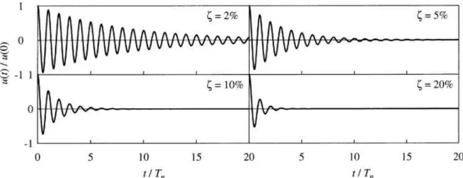
ug(t) . ... 40 Figure 1-2 Free vibration of a SDOF system with different levels of damping:
= , , , and %. (Chopra 2001) ... 41 Figure 1-3 Multiple degree of freedom oscillator (MDOF) subjected to an earthquake ground
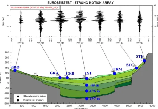
motion ug(t) . ... 43 Figure 1-4 Time histories of the May 13, 1995 earthquake (Ms 6.6, distance 130 km) recorded
on north-south components of stations of the EUROSEISTEST network. (http://euroseisdb.civil.auth.gr) ... 50 Figure 1-5 (a) Geotechnical model of the Mygdonia basin: complete model (top) and simplified
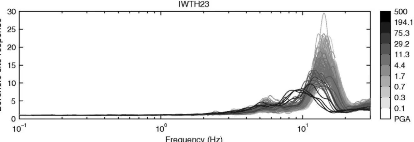
model (bottom), (b) Amplification/frequency curves for various locations along the basin surface for simplified (continuous) and complete models (dashed). (Semblat et al. 2005) ... 50 Figure 1-6 Reduction of the borehole site responses at IWTH23 with respect to the input-motion PGA (cm/s²). (Régnier et al. 2013) ... 51 Figure 1-7 Two-step analyses; step one (left) Free Field analyses and step two (right) Fixed
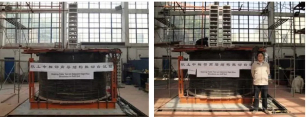
Base analyses. ... 53 Figure 1-8 Photograph of a prototype model for the shaking table test. (Lu et al. 2004) ... 54 Figure 1-9 One-step analysis for SSI problems. ... 57 Figure 1-10 Prototype of a shaking table model scaled to the / , SSI test model (left) and
SSSI test model (right). (Li et al. 2012) ... 59 Figure 1-11 Overview of experiment: (a) single building; (b) two identical buildings; (c) three
identical buildings; (d) experimental system mounted on the shaking table. (Aldaikh et al. 2016) ... 60 Figure 1-12 (a) Prototype and (b) Finite Element Model of two different structures protected
14
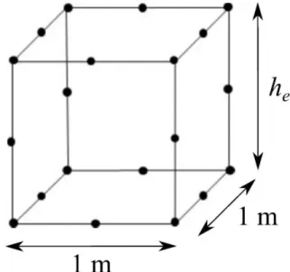
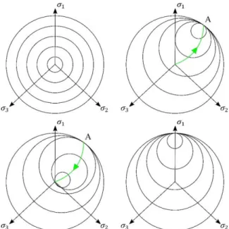
Figure 2-1 Assembly of a frame structure and a multilayer soil domain shaken by a three-component seismic motion, for SSI analysis: (a) 1D-3C wave propagation model, where the assembly is done in only one node; (b) 3D-3C wave propagation model, with connection node-to-node between building and soil; (c) 3D-3C model, where the foundation is modeled and embedded in the soil domain. ... 64 Figure 2-2 Unit area quadratic solid FE with 20 nodes, where ℎ is the element height. ... 65 Figure 2-3 One dimensional series-parallel rheological model proposed by Iwan in 1967. ... 68 Figure 2-4 (a) Shear modulus decay curve and (b) shear strain time history. ... 68 Figure 2-5 Schematic behavior of yield surfaces of Iwan model, in plane. ... 70 Figure 2-6 Yield surface transformation after kinematic hardening (left) or isotropic hardening
(right). ... 70 Figure 2-7 Ratchetting (Abaqus User Manual 2014, Figure 23.2.2–5) ... 70 Figure 2-8 Hysteresis loop in a unit cube of soil obtained with the Fortran implementation of
Iwan’s model (UMAT/SWAP_3C) ... 71 Figure 2-9 Hysteresis loops in a unit cube of soil loaded by a 1-, 2- and 3-Component strain,
for a different number of backstresses in the kinematic hardening model. ... 72 Figure 2-10 Floor plan of the two analyzed three-story buildings that have same (a) and
different (b) inertia to horizontal motion in the two orthogonal directions x and y. The dimensions of the two buildings are the same; the difference is in the rectangular column orientation. ... 75 Figure 2-11 Building base to bedrock Transfer Function, evaluated for different soil areas, and
free-field to bedrock Transfer Function. ... 76 Figure 2-12 NS component of the synthetic seismic signal at the outcropping bedrock, in terms
of normalized acceleration â , for the predominant frequencies q = 2.8 Hz . ... 77
Figure 2-13 Velocity time history (a) and Fourier spectrum (b) for the NS, EW and UP components of the 2009 Mw 6.3 L’Aquila earthquake at recorded ANT station. Dashed lines show the predominant frequency in NS, EW and UP directions. ... 78 Figure 2-14 Acceleration time history at the soil surface, in the case of free-field solution and
15
Figure 2-15 Acceleration time history at the soil surface (top) and at the building top (bottom), in the case of linear soil behavior, for one- (a) and three-component (b) motion. ... 80 Figure 2-16 Parameters associated to lowest GoF scores: (top-left) Response spectrum for the
1C motion in x-direction at the free-field, (top-right) Response spectrum for the 1C motion in x-direction at the building bottom, (bottom-left) Fourier spectrum for the 3C motion in direction at the building bottom (bottom-right) Fourier spectrum for the 3C motion in z-direction at the building top. ... 81 Figure 2-17 Acceleration time history at the soil surface, in the case of free-field solution and
nonlinear soil behavior, for one- (a) and three-component (b) motion. ... 82 Figure 2-18 Acceleration time history at the building base (top) and top (bottom), in the case
of nonlinear soil behavior, for one- (a) and three-component (b) motion. ... 82 Figure 2-19 Simulated acceleration time history at the building bottom in the case of resonance
( = s = 3.8 Hz ) during the input signal duration (top) and in a 10 s time window over the largest amplitudes (bottom). ... 83 Figure 2-20 Simulated acceleration time history at the building top in the case of resonance
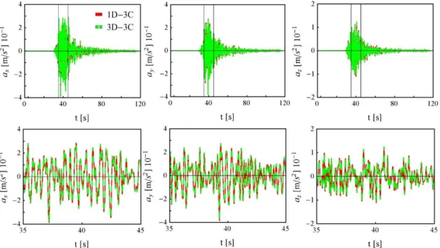
( = s = 3.8 Hz ) during the input signal duration (top) and in a 10 s time window over the largest amplitudes (bottom). ... 84 Figure 2-21 Simulated acceleration time history at the building bottom in the case of SSI
( = 3.8 > s = 2.8 Hz ) during the input signal duration (top) and in a 10 s time window over the largest amplitudes (bottom). ... 87
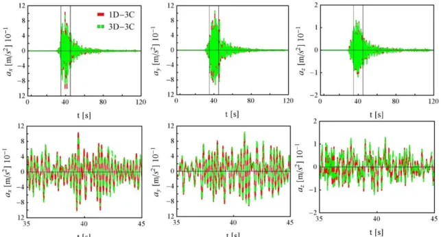
Figure 2-22 Simulated acceleration time history at the building top in the case of SSI ( = 3.8 > s = 2.8 Hz ) during the input signal duration (top) and in a 10 s time
window over the largest amplitudes (bottom). ... 87 Figure 2-23 Horizontal acceleration time history in the cases of soil profile with fundamental
frequency s = b = q = 3.8 Hz , at building bottom (top) and at building top (bottom). ... 88 Figure 2-24 Horizontal acceleration time history in the cases of soil profile with fundamental
frequency s = 2.8 Hz , and b = q = 3.8 Hz , at building bottom (top) and at building top (bottom). ... 89
16
Figure 3-1 Assembly of a multilayer soil domain and a frame structure shaken by a three-component seismic motion: 1D-3C (a) and 3D-3C (b) model for SSI analysis. ... 92 Figure 3-2 Section of the 1DT-3C model for SSI analysis where h is the thickness of the 3-D
soil domain and � is the Thickness of the considered soil until bedrock interface. ... 93 Figure 3-3 1DT-3C model for soil-structure interaction (a) and for structure-soil-structure (b)
analysis. ... 93 Figure 3-4 Maximum shear strain (a) and stress (b) profile with depth obtained using de 1D-3C wave propagation model for the SSI analysis in a linear elastic regime. ... 95 Figure 3-5 Comparison of 1DT-3C and 3D-3C wave propagation approaches for SSI analysis:
acceleration time history at the building bottom (top) and roof drift time history at the building top (bottom). ... 96 Figure 3-6 Comparison of T and 3-D soil models for 1D-3C wave propagation approache for
SSI analysis: energy integral (IE), response spectrum acceleration (Spa) and Fourier spectrum (FS) for the horizontal x-component of motion at the building bottom (top) and top (bottom). ... 97 Figure 3-7 Comparison of T and 3-D soil models for 1D-3C wave propagation approache for
SSI analysis: correlation coefficient of accelerations for the horizontal x-component of motion at the building bottom (a) and top (b). ... 97 Figure 3-8 Acceleration time history at the building bottom (left) and roof drift at the building
top (right), for the building-soil system composed by a T-shaped horizontally layered soil having frequency s = 1.9 Hz and a building having fundamental frequency = 3.8 Hz , in the case of earthquake predominant frequency equal to = s = 3.8 Hz and
= s = 1.9 Hz . ... 98
Figure 3-9 Building top to bottom transfer function estimated for a fixed-base building and for
SSI analysis in the cases of building-soil resonance ( = s = 3.8 Hz ) and softer soil ( = 3.8 Hz > s = 1.9 Hz ). ... 99
Figure 3-10 Acceleration time history at the building bottom and roof drift at the building top, for the building-soil system composed by a building having fundamental frequency
17
(a) and = 1.9 Hz < b = 3.8 Hz (b), in the case of earthquake predominant frequency equal to = b = 3.8 Hz . ... 100 Figure 3-11 Acceleration time history at the building bottom and roof drift at the building top,
for the building-soil system composed by a building having fundamental frequencies b1 = 2.8 Hz and b2 = 4.7 Hz and a T-shaped horizontally layered soil having frequency
s = 1.9 Hz , in the case of earthquake predominant frequency equal to
= b1 = 2.8 Hz . ... 101 Figure 3-12 Acceleration time history at the building bottom and roof drift at the building top,
for the building-soil system composed by a building having fundamental frequencies b1 = 2.8 Hz and b2 = 4.7 Hz and a T-shaped horizontally layered soil having frequency s = 1.9 Hz , in the case of earthquake predominant frequency equal to
= b2 = 4.7 Hz . ... 102 Figure 4-1 2-D section of the 1DT-3C model for SSI analysis where h is the thickness of the
3-D soil domain and � is the Thickness of the considered soil until bedrock interface. ... 106 Figure 4-2 Variation of the peak acceleration at the top of five different buildings, normalized
with respect to the maximum amplitude of the seismic load aq, with the soil fundamental frequency: synthetic signal having predominant frequency close to the building fundamental frequency (left) and 2009 Mw 6.3 L’Aquila earthquake (right) as seismic loading. A vertical dashed line indicates the building fundamental frequency ... 113 Figure 4-3 Variation with the building to soil fundamental frequency ratio of the peak
acceleration at the top of five different buildings, normalized with respect to its maximum: synthetic signal having predominant frequency close to the building fundamental frequency (left) and 2009 Mw 6.3 L’Aquila earthquake (right) as seismic loading ... 114 Figure 4-4 Variation of the peak acceleration at the top of the building in a one-step analysis
over that in a two-step analysis with the building to soil fundamental frequency ratio, for five different buildings: synthetic signal having predominant frequency close to the building fundamental frequency (left) and 2009 Mw 6.3 L’Aquila earthquake (right) as seismic loading ... 115 Figure 4-5 Variation of the peak acceleration at the top of the building in a one-step analysis
18
buildings and a synthetic signal having predominant frequency close to the building fundamental frequency as seismic loading. The ground type range is indicated by vertical boundaries ... 116 Figure 4-6 Variation with the soil fundamental frequency of the peak acceleration at the top of
two buildings having fundamental frequency = 1.5 Hz (left) and = 3.8 Hz (right), in the case of nonlinear behaving soil and nonlinear behaving building-soil system. The synthetic input signal has predominant frequency close to the building fundamental frequency ... 117 Figure 4-7 Variation with the soil fundamental frequency of the peak acceleration, normalized
with respect to the maximum amplitude of the seismic load aq, at the top of two buildings having fundamental frequency = 1.5 Hz (left) and = 3.8 Hz (right), for the cases of linear behaving building-soil system, nonlinear behaving soil and nonlinear behaving building-soil system. The synthetic input signal has predominant frequency close to the building fundamental frequency ... 118 Figure 4-8 Variation with the building to soil fundamental frequency ratio of the peak
acceleration, normalized with respect to the maximum amplitude of the seismic load aq, at the top of two buildings having fundamental frequency = 1.5 Hz (left) and
= 3.8 Hz (right), for the cases of linear behaving building-soil system, nonlinear behaving soil and nonlinear behaving building-soil system. The synthetic input signal has predominant frequency close to the building fundamental frequency ... 118 Figure 4-9 Variation with the building to soil fundamental frequency ratio of the peak
acceleration at the top of two analyzed buildings, normalized with respect to its maximum, for the cases of linear behaving building-soil system (left), nonlinear behaving soil (middle) and nonlinear behaving building-soil system (right). The synthetic input signal has predominant frequency close to the building fundamental frequency... 119 Figure 4-10 Variation with the building to soil fundamental frequency ratio of the peak
acceleration at the top of the building in a one-step analysis over that in a two-step analysis, for the two analyzed buildings, in the cases of linear behaving building-soil system (left), nonlinear behaving soil (middle) and nonlinear behaving building-soil system (right). The synthetic input signal has predominant frequency close to the building fundamental frequency ... 120
19
Figure 5-1 2-D section of the 1DT-3C model for SSI analysis where h is the thickness of the 3-D soil domain and � is the Thickness of the considered soil until bedrock interface. ... 124 Figure 5-2 Simulated acceleration time history of the building with b1 = b2 = 3.8 Hz at the
building bottom, in the case of a nearby building with b1 = b2 = 3.8 Hz , during the input signal duration (top) and in a 10 s time window over the largest amplitudes (bottom). ... 128 Figure 5-3 Simulated acceleration time history of the building with b1 = b2 = 3.8 Hz at the
building bottom, in the case of a nearby building with b1 = 2.8 Hz different than b2 = 4.7 Hz , during the input signal duration (top) and in a 10 s time window over the largest amplitudes (bottom). ... 128 Figure 5-4 Simulated acceleration time history of the building with b1 = 2.8 Hz different than
b2 = 4.7 Hz at the building bottom, in the case of a nearby building with b1 = 2.8 Hz different than b2 = 4.7 Hz , during the input signal duration (top) and in a 10 s time window over the largest amplitudes (bottom). ... 129 Figure 5-5 Simulated acceleration time history of the building with b1 = 2.8 Hz different than
b2 = 4.7 Hz at the building bottom, in the case of a nearby building with b1 = b2 = 3.8 Hz , during the input signal duration (top) and in a 10 s time window over the largest amplitudes (bottom). ... 129 Figure 5-6 Comparison of results obtained using the 1DT-3C wave propagation model for
isolated building and SSSI, in terms of Arias integral (AI), energy integral (IE), pseudo-acceleration response spectrum (Spa) and Fourier spectrum (FS) for the vertical component (z) of motion and s = 2.8 Hz : (a) building with b1 = b2 = 3.8 Hz at the building bottom, in the case of a nearby building with b1 = b2 = 3.8 Hz ; (b) building with b1 = b2 = 3.8 Hz at the building bottom, in the case of a nearby building with b1 = 2.8 Hz different than b2 = 4.7 Hz ; (c) building with b1 = 2.8 Hz different than b2 = 4.7 Hz at the building bottom, in the case of a nearby building with b1 = 2.8 Hz different than b2 = 4.7 Hz ; (d) building with b1 = 2.8 Hz different than b2 = 4.7 Hz
at the building bottom, in the case of a nearby building with b1 = b2 = 3.8 Hz . ... 130 Figure 5-7 1DT-3C for SSSI analysis ... 131
20
Figure 5-8 Variation of the peak acceleration at the top of the excited building with the natural frequency of the nearby building, for the cases of soil profile having natural frequency s = 1.5 Hz (left) and s = 2 Hz (right) ... 132 Figure 5-9 Variation of the peak acceleration at the top of the target building in a SSSI analysis
over that in a SSI analysis (single excited building) with the natural frequency of the nearby building, for the cases of soil profile having natural frequency s = 1.5 Hz (left) and s = 2 Hz (right): excited target building (top); excited nearby building (bottom) 133 Figure 5-10 Variation of the peak acceleration at the top of the target building in a SSSI analysis
over that in a SSI analysis (single excited building) with the target to nearby building fundamental frequency ratio, for the cases of soil profile having natural frequency
s = 1.5 Hz (left) and s = 2 Hz (right): excited target building (top); excited nearby building (bottom) ... 134 Figure 5-11 3-D soil model with semi-infinite lateral elements. ... 135 Figure 5-12 3D-3C modeled using lateral boundary condition as linear dashpots (a) as semi-infinite elements (b). ... 137 Figure 5-15 Comparison between lateral boundary conditions; dashpots and semi-infinite
elements in a 3D-3C FF analysis: acceleration time history at the soil top. ... 138 Figure 5-16 Variation of the soil frequency with the side dimension of the, squared geometry,
21
List of Tables
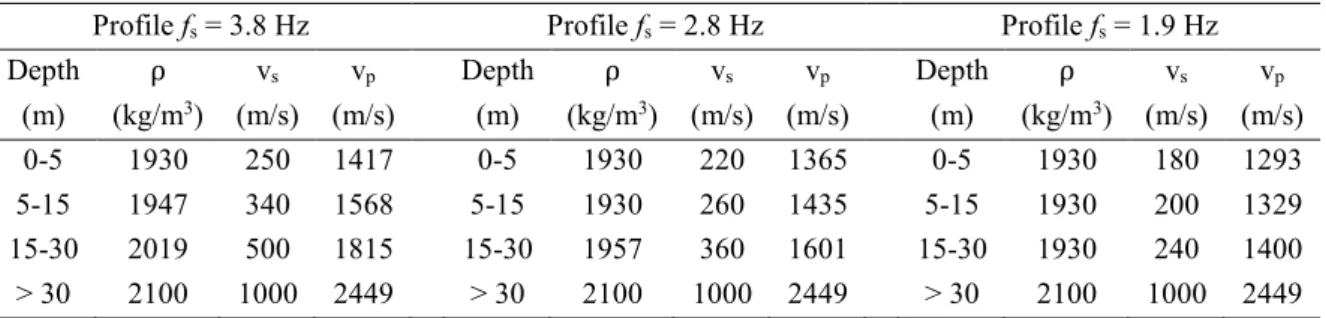
Table 2-1 Stratigraphy and mechanical features of the analyzed multilayered soil profiles having different natural frequency. ... 74 Table 2-2 Dimensions of the rectangular cross-section beams and columns ... 76 Table 2-3 Gof of the 1-D model in the case of linear soil behavior ( = s = q = 3.8 Hz ). 79
Table 2-4 Gof of 1-D model in the case of nonlinear soil behavior ( = s = q = 3.8 Hz ). ... 81 Table 2-5 Gof of 1-D model in the case of nonlinear soil and resonance ( = s = 3.8 Hz ). ... 85 Table 2-6 Gof of 1-D model in the case of SSI ( = 3.8 > s = 2.8 Hz ). ... 86 Table 3-1 Gof of 1DT-3C model, with respect to a 3D-3C model for SSI analysis. ... 96 Table 4-1 Stratigraphy and mechanical properties of the analyzed soil profiles ... 108 Table 4-2 Eurocode ground type and fundamental frequency of the analyzed soil profiles . 109 Table 4-3 Fundamental frequency of the analyzed frame structures ... 110 Table 4-4 Dimensions of rectangular cross-section beams for the analyzed buildings ... 111 Table 5-1 Stratigraphy and mechanical properties of the analyzed soil profiles ... 125 Table 5-2 Eurocode ground type and fundamental frequency of the analyzed soil profiles . 125 Table 5-3 Fundamental frequency of the analyzed frame structures ... 126 Table 5-4 Dimensions of rectangular cross-section beams for the analyzed buildings ... 126 Table 5-5 Gof of 1DT-3C wave propagation model in the case of a building having a nearby
23
First and most importantly, my sincerest gratitude goes to my supervisors, Paola Santisi and Anne Deshamps. I am grateful for their guidance throughout the three years of my thesis, for their patience, professionalism and wisdom. In particular, I am thankful to Paola for introducing me to this research field, for trusting me and for encouraging me.
I would like to thank the members of my thesis committee. Jean-François Semblat and Pierfrancesco Cacciola who kindly accepted to be referees for my thesis and provided their comments and suggestions on my manuscript. I am also thankful for Luca Lenti and Etienne Bertrand, who accepted to be members of my thesis jury.
I would also like to thank my thesis committee, Françoise Courboulex and Fernando Lopez Caballero, for their time and advices.
I thank all the members of the laboratories JAD and Géoazur, for the hangouts and time spent together at lunch and coffee breaks especially my colleagues Bjorn, Stefania, Eduard, Luis, Marcella, Lucrezia, Victor, Laurence, Giulia, Mehdi, Léo, Kevin, Alexandre, Alxis G., Alexis L., David M., Théa, Zoé, Alexianne, Nicolas, Emmanuelle, Mathilde, Laure, Sara, Jean-luc, Simon and David C. Also, I am thankful to my co-office David L. and Julie we’ve shared so much together.
I want to thank Jean Marc Lacroix for his enormous help, I have learned a lot from him about clusters and codes.
I am also grateful to my friends Roula, Rita, Michelle, Rachelle, Christelle, Farah, Ralph, Tina and Joseph who have been there for me every time. Of course, special thanks to my F.R.I.E.N.D.S for their sense of humor.
My deepest appreciation goes to my father Milad, my mother Amal, my sisters Joelle and Nathalie and brothers in law François and Rami for their support, their prayers and their visits. Finally, this research is performed using HPC resources from GENCI-[CINES] (Grant 2017-[A0010410071] and Grant 2018-[A0030410071]). This work has been funded by the region Provence-Alpes-Côte d'Azur (South-Eastern France), through a doctoral fellowship, and by the CNRS, through the project PEPS de site 2016 CNRS Université Nice Sophia Antipolis entitled “SSSI effects in the seismic response: identification of mechanical properties of buldings using M‐MS and 3D modeling”.
25
Dedicated to my beloved family Milad, Amal, Joelle and Nathalie
27
Résumé étendu
Mon travail s’intéresse à la réponse sismique des structures dans leur environnement. Cette réponse sismique d'une structure dépend de la secousse incidente et de la propagation des ondes dans le sol et dans la structure elle-même. La structure étant couplée mécaniquement au sol, son excitation renvoie les ondes dans le sol. Ce phénomène est l’Interaction Sol Structure (ISS). Selon les codes européens de conception parasismique en vigueur (CEN 2003), le mouvement en surface libre est actuellement utilisé comme chargement sismique au bas d'un bâtiment à base fixe (BF), pour la conception de bâtiments à fondation superficielle. Cette analyse en « deux étapes » (Saez et al., 2011), ne permet donc pas de simuler numériquement l’ISS. Les effets d’ISS ne sont pris en compte que lorsque la réponse sismique de la structure est obtenue en résolvant le problème de l'équilibre dynamique appliquée à l'ensemble du domaine sol-structure : analyse en une étape. Nous avons montré que l’on pouvait, dans certaines conditions, considérer les effets de l’ISS comme une modification de la sollicitation sismique, influencée par les caractéristiques dynamiques structurelles, les paramètres mécaniques du sol et les caractéristiques de mouvement d'entrée.
Lors d’une sollicitation sismique, la topographie, la caractérisation géologique et géomécanique du sol affectent de manière significative le mouvement enregistré à surface libre. ‐n particulier, de plus en plus les études s’attachent à comprendre les effets d’un comportement mécanique non linéaire dans les couches superficielles, comme dans les structures. Ces effets sont mis en évidence par exemple lors du benchmark PRENOLIN (Régnier et al. 2016) au cours duquel plusieurs relations constitutives non-linéaires ont été comparées par simulation numérique de la réponse sismique non-linéaire de site 1-D. Mais ces modèles testés exigent un nombre de paramètres important pour correctement reproduire la réponse du sol à un niveau de charge élevé. Comme pratiquement ces paramètres de sol peuvent être difficiles à déterminer, ces modélisations, importantes pour la compréhension des phénomènes, sont impossibles à introduire dans la règlementation. Je me suis attachée à concevoir un système équivalent plus simple : un modèle constitutif de sol efficace est celui qui est fiable et nécessite peu de paramètres à caractériser.
Plus largement, lorsque la construction est étendue à plus d'une structure, l’excitation sismique d’une structure est affectée par la présence des structures adjacentes. Cette interaction croisée entre structures voisines et le sol lors d’une sollicitation sismique est appelée interaction
28
structure-sol-structure (ISSS). Nous avons aussi abordé cette question fondamentale dans la construction des villes.
Afin d’étudier l’ISS et l’ISSS, une modélisation numérique du système sol-structure sous un chargement sismique est nécessaire. Plusieurs méthodes numériques ont été utilisées pour résoudre la propagation de l’onde dans un environnement complexe : les différences finies, les éléments finies (EF), les éléments spectraux, les éléments frontières et d’autres. Selon Chaljub et al. (2010), aucune méthode numérique unique ne peut être considérée comme la meilleure. Dans mon travail, la solution directe de l'équation d'équilibre dynamique est résolue dans un schéma EF et le comportement non-linéaire des matériaux est pris en compte. Des conditions aux limites latérales périodiques sont adoptées, pour réduire le domaine du sol modélisé, lorsque l'hypothèse de périodicité est possible. Les résultats obtenus me permettent de proposer un modèle efficace pour la pratique de l’ingénierie qui tient compte de l’ISS.
Modèle de propagation unidimensionnel d’onde à trois composantes pour l’interaction sol-structure
Pour mettre en œuvre la simulation, un modèle de propagation unidirectionnelle (1D) est couplé à un modèle de bâtiment tridimensionnel (3-D) dans l’hypothèse de propagation d’onde verticale et de fondation superficielle rigide (modèle 1D-3C). Cette formulation est adaptée à la description de la colonne de sol par les données géotechniques généralement disponibles et permet de réduire le temps de calcul. Il est encore assez rare de connaître la géométrie et la stratigraphie d’un bassin sédimentaire qui serait nécessaire à une modélisation 3-D plus complète.
La loi de comportement d’Iwan (Iwan 1967), a été utilisée pour décrire le comportement non linéaire du sol sous chargement cyclique, en termes de contraintes totales. La solution du problème d’ISS est obtenue par solution directe de l’équation d’équilibre dynamique de l’ensemble. L’hypothèse de sol infiniment étendu dans les directions horizontales est traduite par une condition de périodicité latérale. Le mouvement sismique est imposé à la base de la colonne de sol en utilisant une condition absorbante qui prend en compte l’effet de l’élasticité du substratum rocheux.
Le modèle 1D-3C a été vérifié, dans le cas de comportement linéaire de sol et en utilisant un algorithme d’intégration implicite, par comparaison avec les résultats obtenus par le code maison SWAP_3C (Santisi d’Avila and Lenti 2012) pour les études de réponse sismique du
29
sol à la surface libre et S‑RINT_3C (Santisi d’Avila and Lopez-Caballero 2018) pour les études de réponse sismique de sol et du bâtiment en considérant l’ISS. ‐nsuite, le modèle 1D-3C est validé, dans le cas de comportement non-linéaire de sol.
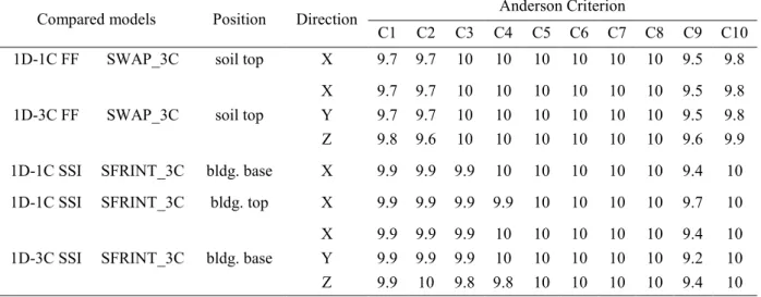
L’objectif est de prouver la pertinence du modèle de propagation 1D-3C dans un problème d’ISS, comparé à un modèle 3D-3C. Conceptuellement, ce dernier donne l’avantage de pouvoir modéliser la dalle de fondation par des éléments finis solides et donc de prendre en compte sa déformabilité. Par contre, dans le modèle de propagation 1D-3C, le même mouvement est imposé à la base de tous les poteaux du bâtiment simulant une base rigide. La comparaison quantitative des signaux obtenus par le modèle 1D-3C est effectuée en termes de pics en amplitude, d’intégrale d’Arias, d’intégrale en énergie, de spectre de ‑ourier et de réponse et de rapport de corrélation (coefficients du comparatif Goodness-of-fit proposés par Anderson, 2004). Les résultats obtenus dans le cas de propagation verticale montrent la fiabilité du modèle 1D-3C pour le sol quand les hypothèses de couches horizontales suffisamment étendues et de fondation superficielle rigide sont respectées. Le cas d’un champ d’onde incliné fera partie d’une étude ultérieure.
Propagation unidirectionnelle d'onde à trois composantes dans un domaine de sol en forme de T pour l’ISS et l’ISSS
L'approche de propagation unidirectionnelle d’une onde à trois composantes (1D-3C) est adoptée pour résoudre la réponse dynamique du sol. La technique de modélisation de propagation unidirectionnelle d'une onde trois composantes est étendue pour des analyses d'ISS et ISSS. Les résultats obtenus sur l’ISS montrent que cette interaction n’est observée dans le sol que dans les premières couches. Par conséquence, un modèle de sol 3-D est adopté jusqu'à une profondeur fixée, au-dessus de laquelle on considère que la déformation est influencée par l’ISS et l’ISSS, alors qu’un modèle de sol 1-D est adopté pour les couches de sol plus profondes, jusqu'à l'interface sol-substrat (modèle 1DT-3C). Le profil de sol en T est assemblé avec une ou plusieurs structures 3-D de type poteaux-poutres à l’aide d’un modèle par éléments finis, pour prendre en compte, respectivement, l’ISS et l’ISSS. Ce modèle permet de prendre en compte la déformabilité de la fondation et les effets de basculement et peut simuler l’interaction entre plusieurs bâtiments.
L'approche 1DT-3C est vérifiée par comparaison avec un modèle entièrement 3D-3C, dans le cas d'une propagation verticale dans un sol stratifié horizontalement. La technique de
30
modélisation 1DT-3C proposée est donc un outil pour la conception de bâtiments, permettant de prendre en compte l’ISS de manière efficace et simple. De fait, dans le cas d’une propagation verticale et de paramètres géotechniques homogènes dans chaque couche de sol, l’utilisation d’éléments solides unitaires pour les couches plus profondes, au lieu d’un domaine 3-D, représente une réduction du temps de calcul sans affecter les résultats.
L’effet d’ISS est défini comme la différence en termes d'accélération maximale a _ /a _ entre la solution en une étape (résolution directe du problème d’équilibre dynamique de l’ensemble sol-bâtiment) et la solution obtenue par la méthode en 2 étapes (mouvement à surface libre appliqué à un bâtiment à base fixe). Mon étude montre que cet effet est plus important dans le cas où le sol est plus mou et dans le cas d'un comportement de sol non linéaire. Des effets de résonance entre les fréquences du bâtiment, la fréquence associée au sol et le contenu fréquentiel du signal sismique produisent une réponse sismique amplifiée. L'effet d’ISS est observé pour les deux premiers modes de translation du bâtiment et est plus prononcé dans la direction du mode excité par la charge d'entrée.
Spectre de réponse pour la conception parasismique tenant compte de l'interaction sol-structure
Une analyse paramétrique de la réponse sismique des bâtiments en béton armé est développée et discutée pour identifier les paramètres clé du phénomène d’ISS, influençant la réponse structurelle, à introduire dans la conception parasismique de bâtiments.
La variation de l'accélération maximale en haut du bâtiment avec le rapport de fréquence bâtiment / sol est tracée pour plusieurs bâtiments, chargés par un mouvement à bande étroite qui excite leur fréquence fondamentale. Dans le cas de sols et de structures à comportement linéaire, une tendance similaire est obtenue pour différents bâtiments. En régime élastique linéaire, l’ISS peut être pris en compte à l'aide d'un facteur de correction appliqué au résultat d'une analyse en deux étapes (modèle de bâtiment à base fixe chargé par un signal sismique à surface libre). Ce facteur de correction dépend du rapport de fréquence fondamentale / du bâtiment au sol.
L'analyse paramétrique est répétée en introduisant l'effet de la non-linéarité du sol et du béton armé. L'effet de la non-linéarité du sol sur la réponse sismique des bâtiments est prépondérant par rapport à l'effet de la non-linéarité du béton armé. La non-linéarité du comportement du sol ou du sol et de la structure, tend à augmenter l'irrégularité de la réponse sismique des bâtiments.
31
De plus elle modifie la fréquence de vibration pendant le processus. Par conséquent, en tenant compte du comportement non-linéaire des matériaux, la réponse sismique des bâtiments considérant l’ISS ne peut plus être reproduite en appliquant un simple facteur de correction sur les résultats obtenus par l’analyse en deux étapes.
Analyse de l'interaction structure-sol-structure
La réponse sismique d'un bâtiment en béton armé est estimée en tenant compte de l'effet d'un bâtiment voisin, pour un sol et des structures à comportement linéaire. Cette approche permet une analyse efficace de l'interaction structure-sol-structure pour la pratique de l'ingénierie afin d'inspirer la conception d'outils pour la réduction du risque sismique et l'organisation urbaine. L'analyse effectuée à l'aide de la technique de modélisation 1DT-3C montre que l’ISSS est observée dans la direction du premier mode de vibration du bâtiment. L’ISSS donne, pour certains cas, une amplification jusqu’à % du mouvement non prise en compte lorsque le bâtiment est considéré comme isolé. En outre, dans un sol meuble, la réponse sismique du bâtiment excité ne présente pas de variations importantes du fait de la présence de bâtiments voisins. L’effet de l’ISS l’emporte sur l’effet de l’ISSS.
Conclusions et perspectives
Dans les pratiques professionnelles, les normes de conception évoluent en fonction des nouvelles découvertes et des progrès croissants les capacités informatiques. Aujourd'hui, les codes de conception sismiques européens ne prennent toujours pas en compte l’ISS et l’ISSS dans la conception des structures. Cette recherche étudie les phénomènes d’interaction entre sol et structures, propose et valide des techniques de modélisation pour évaluer les réponses dynamiques des sols et des structures aux séismes, en prenant en compte l’ISS et l’ISSS. L'approche de propagation des ondes sismiques 1DT-3C est proposée comme technique de modélisation pour la simulation de la réponse sismique des sols et des bâtiments, en tenant compte des effets de site, de la déformabilité des fondations, des effets de basculement et, éventuellement, de l’ISSS. Le modèle 1DT-3C consiste à adopter un modèle entièrement 3-D jusqu'à une profondeur fixe, au-dessus de laquelle les effets d’ISS et d’ISSS modifient le mouvement du sol et au-delà de laquelle un modèle 1-D est supposé être une approximation suffisante.
32
La technique de modélisation 1DT-3C proposée est un outil efficace pour la conception de bâtiments, permettant de prendre en compte facilement et efficacement les ISS et ISSS pour des comportements des matériaux linéaires et non-linéaires, offrant des avantages en terme de temps de modélisation et de calcul par rapport à un modèle entièrement 3-D. L’introduction des comportements non-linéaires est absolument nécessaire car les observations actuelles dans les zones soumises à de fortes sollicitations sismiques, montrent que ces effets sont importants. Par ailleurs cet outil s’adapte bien aux pratiques :
- les paramètres géotechniques peuvent assez simplement caractérisés pour un modèle de sol unidimensionnel en utilisant un forage, alors qu’une caractérisation 3D serait très lourde (plusieurs forage et mise en adéquation des observations).
- la définition des conditions aux limites est simple : le signal d'entrée et la condition aux limites d'absorption ne sont donnés que pour un seul élément.
- le maillage est considérablement réduit.
L’analyse paramétrique combinant 11 profils de sol et 5 structures différentes montre qu’en régime élastique linéaire l’ISS peut être pris en compte assez facilement à partir des résultats d’une étude traditionnelle en deux étapes. Elle permet donc de proposer une amélioration potentielle des spectres de réponse pour la conception parasismique proposés par l’‐urocode 8 en régime élastique.
Par contre le comportement non-linéaire du matériau provoque une modification de la réponse sismique du sol et des bâtiments, avec en particulier, une modification les fréquences caractéristiques. L’analyse paramétrique que je présente permet de tirer quelques résultats qualitatifs, mais montre qu’il n’y a pas de façon simple, pour la conception des bâtiments, de s’appuyer sur les modélisations traditionnelles qui se limitent à un comportement linéaire des matériaux.
La méthode proposée est efficace aussi pour une analyse de l'influence de l’ISSS sur un bâtiment cible. Je présente une analyse paramétrique le régime élastique linéaire. Les résultats montrent que si, dans le cas de sol mous, l’effet de l’ISS l’emporte sur l’effet de l’ISSS, dans les autres conditions de sol l’ISSS ne peut pas être négligé. L'analyse paramétrique donne des résultats préliminaires qui ne permettent pas encore de généraliser.
Cette recherche pourrait se prolonger par une analyse paramétrique et une étude statistique approfondies visant à généraliser la conception des structures dans les zones sismiques, en tenant compte des effets d’ISS. Pour permettre la vérification du modèle numérique, des
33
expériences sur des structures instrumentées à des échelles réelle ou proportionnelle pourraient être utilisées pour comparer observations et calculs numériques. L'approche de propagation des ondes 1D-3C pourrait évoluer pour modéliser les fondations profondes et les sols encaissants, en considérant un domaine 3-D atteignant une plus grande profondeur. Une analyse de contrainte efficace, prenant en compte la position de la nappe phréatique dans un modèle de propagation d'ondes 1DT-3C pour l’analyse de l’ISS, est actuellement développée dans le cadre de la thèse de doctorat de Stefania Gobbi. D'autres améliorations peuvent être introduites comme, la corrosion des barres d'acier dans le béton armé ou la considération des matériaux de construction différents tel que le bois et l’acier.
35
Introduction
Earthquake engineering research is an interdisciplinary field involving structural and geotechnical engineers, seismologists, architects and urban planners. It is a discipline that studies the antiseismic conception of new structures and the ability of existing structures to survive an earthquake without sever damage. The building codes are based on actual knowledge concerning the seismic conception and design.
The need for such codes is initiated by several major earthquake disasters causing damage to structures hence, to population. The damage concerns reinforced concrete structures as well as wooden and steel structures and is observed in low-, mid- and high- rise buildings and that, either in lower, mid or upper story of structures. Earthquake damage also attains the soil leading to soil failure and eventual the collapse of the structures.
Due to variabilities in observations and seismic risk in regions the requisite for research in this field becomes higher in order to understand soil and structure responses to earthquakes and contribute in the progress of seismic codes. There are several seismic codes used in the world, most of them share similar fundamental design approaches and only differ in the techniques of application regarding local geological conditions and common new and old construction types. In France the first text aiming to prevent constructions to earthquake shakings was written in 1955 in the recommendation AS55. The text was updated through time with studies and new earthquake events. In 2005 the Eurocode 8, a new seismic code based on the European rules for construction, is employed in France to protect people and restrain structural damages to earthquakes. The metropolitan France presents moderated seismicity in which the eastern Provence presents the highest risk. For this reason, the region of Provence-Alpes-Côte d'Azur encourage research on seismic risk in the purpose of prevention of structural seismic damages. Previous researches have shown that the interaction between the soil and the building induces modification in the dynamic response of the building (Veletsos and Meek 1974; Jennings 1970; Wolf 1985; Gazetas 1991). This modification of the structure response is not beneficial in all conditions and if it is the case, an overdesign is assumed.
The soil-structure interaction (SSI) has been the subject of many works, showing the importance of the SSI assessment in seismic structural design. In the Eurocode 8 the structure is considered as a simplified model using single degree of freedom (SDOF) and SSI is studied in a two-step analysis as named by Saez et al. (2011). This two-step analysis doesn’t correctly model the interaction between the soil and the structure. An update to such procedure
36
considering the advances in theory and practice is mandatory. The lack of the previous version of the Eurocode 8 has encourage this research to consider SSI for structures with shallow foundation, model multilayered soil profiles and study the dynamic response of the assembly soil-structure.
The Eurocode 8 is limited to the elastic linear behavior of materials. However, evidence of nonlinearity in the soil has been observed for a long time now. In Japan, a seismological data is recorded in Kiban Kyoshin Network since 1995, following the Hyogo-Ken Nanbu earthquake of 1995 Kobe Japan, and provides evidence that soils tend to quickly reach nonlinearity properties for higher shaking amplitude. On the other hand, a non-cracked structure is an overstatement, cracks are created in concrete at early age and nonlinear behavior of the reinforced concrete should be considered to study the seismic response of a structure. The aim of this research is to provide additional knowledge on structure and soil seismic responses, evaluate the accuracy of modeling techniques employed to replicate the SSI effect due to dynamic excitation and propose eventual advancement in the earthquake engineering field.
The progression of this research goes as following:
• Modeling technique for SSI (Chapter 2): The one-directional three-component (1D-3C) wave propagation approach is propagated in a one-dimensional (1-D) soil assembled with 3-D frame structure in a finite element (FE) scheme (1D-3C). The linear elasticity is employed, it is a simplification considered for structural design, assuming a behavior in elastic strain range, sufficiently far from yielding threshold. This hypothesis simplifies the numerical computations, avoiding modeling of nonlinear material behavior, accepting superposition principle and modeling concrete as a homogeneous material before cracking without the effect of reinforcing bars. Later the nonlinear behaving of materials is considered, in a dynamic analysis, introduces the hysteretic dissipation of energy in the assembly soil-structure and the system soil response is modified and depends on more parameters and on the time history, increasing the difficulty of prediction with simplified empirical tools.
The 1D-3C model is verified comparing with validated codes in a free field (FF) analysis using SWAP_3C (proposed by Santisi d’Avila and Lenti 2012), and in a SSI analysis using S‑RINT_3C (proposed by Santisi d’Avila and Lopez-Caballero 2018), considering
37
linear and non-linear soil behaving. Analysis are undertaken using the 1D-3C model for SSI analysis.
• Advanced modeling technique for SSI and structure-soil-structure interaction (SSSI) (Chapter 3): Analysis using the 1D-3C model for SSI have shown evidence of the effect of SSI in the first layers of the soil and negligible or no effect in deeper soil. Based on this observation a T-shaped soil modeling is proposed (1DT-3C). It consists on modeling 3-D soil model until a certain thickness to be defined, depending on the SSI, connected to a 1-D soil modeled until the bedrock interface. The 3-D soil model permits the embedment of a 3-D foundation connected to the base node of the columns of the 3-D structure allowing rocking effect. The 1DT-3C present an efficient modeling technique for engineering practice, to consider SSI in any commercial FE code.
The proposed 1DT-3C model is verified, in linear and non-linear soil behaving, and SSI analysis are undertaken.
• Parametric investigation on SSI (Chapter 4): After verification of the proposed model for dynamic SSI and SSSI analyses, different computations are carried out to compare the structure and soil responses to earthquake, in the cases of linear and nonlinear behaving materials. A parametric analysis is performed to investigate the variation of the SSI effect with soil and structure dynamic features of the frequencies.
• Parametric investigation on SSSI (Chapter 5): Afterward a study on SSSI is held focusing on a target building and varying the nearby building and quake predominant frequency. The lateral boundary condition is investigated in order to assess a complex geometry of soil and structure plan for SSSI investigations.
39
Chapter 1 -
Overview on soil and structural dynamics
Continuous efforts have been made towards improving modeling techniques in earthquake engineering (characterization of geotechnical parameters, rheologic behavior, site effects, interaction between structure and soil, and with nearby structures), beside the continuous development of risk mitigation tools. Moreover, design codes need to evolve in the regulation of seismic loading definition using signals. Numerical methods that solve a dynamic soil-structure interaction problem is not currently adopted in the engineering practice for building design, but it remains a subject for researchers or taken into account in design of bridges, dams or towers. In the following, basic concepts of structural dynamics are introduced and previous research findings are presented.
1.1 Introduction to structural dynamic problem
40
1.1 Introduction to structural dynamic problem
In structural analysis, static and dynamic loading are considered. If the applied load has a long period, enough to be consider constant and neglect inertial forces it is static otherwise it is a dynamic load.
The structural dynamics aims to study the behavior of a structure under dynamic loadings. In particular, in earthquake engineering the structural response to earthquakes is analyzed. 1.1.1. Single degree of freedom (SDOF)
An adopted simplification to model structures under seismic loading is to represent the structure using a single degree of freedom oscillator (SDOF). It consists on a lumped mass held by a massless column with stiffness , damping coefficient (Figure 1-1). The system is considered fixed at the bottom and subjected to earthquake loading, = − � , that is time dependent, according to Newton’s second law, where � is the ground acceleration at the building base. The differential equation of motion for the SDOF oscillator is
+ + = (1-1)
where , , and are the inertial, viscous and elastic force, respectively. The dot represents time derivative and , and are the structural displacement, velocity and acceleration, respectively.
Figure 1-1 Single degree of freedom oscillator (SDOF) subjected to earthquake ground motion
(t) .
41
+ w + = − � (1-2)
where � is the seismic loading, = ⁄ is the damping ratio, = is the critical damping coefficient and = √ ⁄ is the undamped angular frequency of the oscillator (Chopra 2001). The solution of the homogenous equation of motion (− � = having initial static conditions = , = is written in
= e_ζ 0 [ cos + + ⁄ sin ] (1-3)
where = √ − ². The natural period of the oscillator is � = ⁄ its frequency is = ⁄ implying that more the structure is stiffer, higher is its natural frequency of � vibration.
The increase of the damping ratio in Eq. (1-2) outcomes a slow to fast attenuation of the free vibration (Figure 1-2). Damping in structures originate from a low friction in materials but it is mostly due to damage in non-structural elements (Bachmann et al. 2012). The typical damping for buildings vary between and %, this implies that the damped and undamped natural period and frequencies are almost identical.
Figure 1-2 Free vibration of a SDOF system with different levels of damping: = , , , and %. (Chopra 2001)
1.1 Introduction to structural dynamic problem
42
1.1.2. Numerical solution of the dynamic equilibrium equation for SDOF oscillators
The dynamic equilibrium equation for a SDOF oscillator under seismic loading � is written in Eq. (1-2), it can be rewritten as
= � Δt − + � Δt − + � Δt (1-4)
= � + (1-5)
where the subscript is the iteration step, = − � and
= [ ] (1-6)
Eq. (1-4) and Eq. (1-5) can be solved by iteration, considering the static initial conditions = , = . The variables � Δt , , , � Δt and � Δt in Eq. (1-4) and Eq. (1-5) are defined as following
� Δt = [− Δt ℎ Δt
− ℎ Δt ℎ Δt ], = [ ], = [− − ]
(1-7)
� Δt = � Δt − Δt /Δt − , � Δt = Δt /Δt − � − (1-8) where the functions presented in Eq. (1-7) and Eq. (1-8) are defined as
Δt = � Δt − � − (1-9)
Δt = − / −ζ 0Δ cos Δ + / sin Δ (1-10)
ℎ Δt = − / −ζ 0Δ sin Δ (1-11)
ℎ Δt = −ζ 0Δ cos Δ − w / sin Δ (1-12)
1.1.3. Dynamic study of a MDOF system in the frequency domain
The dynamic solution of a multiple degree of freedom (MDOF) structure under seismic loading � t , assuming linear constitutive behavior of materials, is written as
43
+ + = − �u� (1-13)
where the , and are the mass, stiffness and damping matrices respectively. The dot represents the time derivative, consequently, , and are the displacement, velocity and acceleration vectors, respectively, and � is the influence vector.
Under the assumption of lumped mass, the structural model is simplified as in Figure 1-3 and the mass matrix is diagonal as = diag{ , … } , where the subscript represents the total number of stories in the building.
Figure 1-3 Multiple degree of freedom (MDOF) oscillator subjected to an earthquake ground motion (t) .
The modal analysis can solve the dynamic equilibrium of a multiple degree of freedom MDOF system under the assumption of structural response resulting from the superposition of mode shapes. This, under the hypothesis of linear behaving materials. The dynamic equilibrium equation Eq. (1-13) can be written in modal coordinates by imposing the transformation
= ��. Accordingly, it is
�� + �� + �� = − � � (1-14)
where � is the modal displacement at the time step and � is the modal matrix compound by the eigenvectors obtained by solving
1.1 Introduction to structural dynamic problem
44
� = �� (1-15)
The natural angular frequencies are obtained as solution of
det − � = (1-16)
where � is the vector of eigenvalues such that � = and �� = { }. Each � corresponds to the squared angular frequency of the structure such that < < ⋯ < . The subscript represents the jth mode shape.
The modal transformation corresponds to an operation of diagonalization of matrices , and . Consequently, the dynamic equilibrium equation for the MDOF system in Eq. (1-14) is solved as a system of independent dynamic equilibrium equations of SDOF systems
� + �� + � � = −�� �Δu
� (1-17)
where � = ���{ } and the modal matrix must be orthonormal with respect to the mass matrix and satisfy �� � = � and �� � = � . Each one of Eq. (1-17) is solved as explained in section 1.1.2, since the analytical solution is known for the SDOF. The modal superposition is possible only for linear behavior of materials and proportionally damped structures.
1.1.4. Dynamic equilibrium for MDOF structures
In the case of nonlinear behaving materials, i.e. when the stress-strain relationship is nonlinear, the dynamic equation is
+ + = − �Δu� (1-18)
where the stiffness and damping matrices vary during the process.
Time discretization is needed in order to solve this problem. According with the -method (Hughes 1987), at each time step the following equation can be resolved
+ + + + − − −
− − − = + Δ − Δ − (1-19)
45
+ + + + − − − − − −
= + Δ − Δ − (1-20)
The increment of velocity and acceleration at time step are written in function of the increment of displacement , as following, and substituted in the Eq. (1-20)
= γ/ Δt − γ/ − + − γ/ Δt − = / Δt − / Δt − + / Δt −
(1-21)
at each time step, the displacement increment is obtained by modified equilibrium equation
̅ = + − (1-22)
where the modified stiffness matrix is
̅ = / Δt + + γ/ Δt + + (1-23)
and the vector − is dependent on the result of the previous time step and calculated as
− = [ / Δt + + γ/ ] −
+[ / + + γ/ − Δt ] −
+ − − + − − − Δ −
(1-24)
After evaluating the increment of displacement using Eq. (1-22), the increment of velocity and the increment of acceleration are calculated using Eq. (1-21). The total displacement , velocity and acceleration are then deduced as
= − + = − + = − + (1-25)
The derivation introduces high frequency noise into the solution; numerical damping removes this high-frequency noise without having any significant effect on the meaningful, lower frequency response. The control over the amount of numerical damping is provided by the
-method using the parameters , = . − and = . − such that − / (Hughes 1987).
The Newmark algorithm is obtained for = , using . in the case of unconditional stability.
1.2 Numerical methods
46
1.2 Numerical methods
A numerical method is evaluated according to its efficiency, in terms of time, computer memory, and accuracy. According to Chaljub et al. (2010), no single numerical method can be considered as the best. Several methods have been used to solve wave propagation in media; finite difference method (FDM), boundary element method (BEM), spectral element method (SEM) and standard finite element method (FEM).
PRENOLIN benchmark (Régnier et al. 2016) has compared 20 codes with different numerical scheme and found a standard deviation in results of 0.065 in logarithmic unit for a low-frequency input motion at low PGA values, this deviation increases with the PGA but this may also be due to the differences in the nonlinear model implementation. In this paragraph four different numerical modeling methods are selected to be presented along with their advantages and disadvantages, that often depend on the application.
1.2.1 Finite difference method
The FDM has a long tradition in seismology and geophysics. It consists on replacing the partial derivatives by divided differences or combinations of point values of the function in a finite number of discrete nodes of the regular mesh (Moczo et al. 2004).
Considering , , , a function in space and time. The approximation of the derivative, according to Taylor series of order one, is
� , , , /� ≈ [ + Δ , , , − , , , ]/Δ + � Δ (1-26) Where � Δ is the error due to the approximation.
The FDM has been employed in SEISMOSOIL http://asimaki.caltech.edu/resources/index. html#software) for analysis and signal processing of 1-D site-specific response problems, by Li and Assimaki (2010) using a modified hyperbolic soil model, in NOAH (Bonilla 2001), for wave propagation in saturated soil subjected to vertically incident ground motion and by Moczo et al. (2004) in an adjusted finite difference approximation.
The advantages that present this method are the simplicity of modeling and its low cost in computer memory. However, this method presents as inconvenient the limitation in representing a complex geometry as heterogeneity and topography. The regularity of the mesh,