HAL Id: inria-00591076
https://hal.inria.fr/inria-00591076
Submitted on 6 May 2011
HAL is a multi-disciplinary open access
archive for the deposit and dissemination of
sci-entific research documents, whether they are
pub-lished or not. The documents may come from
teaching and research institutions in France or
abroad, or from public or private research centers.
L’archive ouverte pluridisciplinaire HAL, est
destinée au dépôt et à la diffusion de documents
scientifiques de niveau recherche, publiés ou non,
émanant des établissements d’enseignement et de
recherche français ou étrangers, des laboratoires
publics ou privés.
A dedicated Compression Scheme for Large
Multidimensional Functions Visualization
Matthieu Haefele, Florence Zara, Guillaume Latu, Jean-Michel Dischler
To cite this version:
Matthieu Haefele, Florence Zara, Guillaume Latu, Jean-Michel Dischler. A dedicated Compression
Scheme for Large Multidimensional Functions Visualization. 1st International Workshop on Super
Visualization (IWSV08), Jun 2008, Ile de Kos, Greece. �inria-00591076�
A dedicated Compression Scheme for Large
Multidimensional Functions Visualization
M. Haefele
IRMA, UMR CNRS 7501 Université Louis Pasteur Strasbourg, F-67084, France [email protected]
F. Zara
LIRIS, UMR CNRS 5205 Université Lyon 1 Villeurbanne, F-69622, France [email protected]G. Latu and J-M. Dischler
LSIIT, UMR CNRS 7005 Université Louis Pasteur Illkirch, F-67412, France
ABSTRACT
Large hyper-volume visualization is required by today physic and is still a research area in scientific visualization. Espe-cially, the interactive exploration of datasets remains highly challenging as soon as the data size exceeds a certain thresh-old. We describe in this paper an hyperslicing-based inter-active visualization technique designed to explore at real-time frame rates large hyper-volumetric 4D scalar fields (i.e. datasets beyond 16GB) defined on regular structured grids. The key issue consists in coupling the visualization with a new efficient data representation scheme, in such a way that it overcomes the different steps of scientific visualiza-tion, namely simulation post-processing, visualization pre-processing and finally interactive display. By introducing a hierarchical finite element representation, we show that our technique allows users to explore the full dataset at real-time frame-rates on low-end PCs. We demonstrate the effective-ness of our technique on the interactive exploration of 4D phases space particle beams, resulting from numerical semi-Lagrangian simulations.
1.
INTRODUCTION
In many scientific domains (physics, astronomy, biology, etc.), there are more and more numerical simulations gen-erating huge amounts of complex numerical values, usually dense, multidimensional, multivariate and multi-scale time-varying. This constant evolution induces an increasing de-mand on efficient tools to help users to explore, analyze and visualize such large and densely sampled sets. More-over, multidimensional dataset (with a dimension higher than three) are particularly challenging because of (1) huge amounts of memory requirements, and (2) no easy way to display such a complex information.
Many work in multidimensional visualization has already been driven. We can roughly classify them into two main categories according to the type of data they deal with: mul-tidimensional relation visualization and multidimen-sional function visualization. Multidimenmultidimen-sional relation
visualization can be considered as database visualization, where a record of the database is considered as a multi-dimensional point. In [11], a survey of multimulti-dimensional relation visualization methods is presented.
In this paper, we are concerned with the second category: the multidimensional function visualization and in particu-lar, scalar functions f defined as:
f : Rd → R
x 7→ f (x),
with x = (x1, ..., xd). Most visualization techniques have
given up displaying the whole information at once and only display subsets of the information. With dedicated inter-faces, users can then select these subsets interactively. In all cases, serious visualization problems arise when datasets are large because of core memory limitations and slow data accessibility. Since, these methods strongly resort on inter-activity, real-time performance is a crucial issue.
The curse of the dimensionality arises when functions are defined on a regular discretization of the multidimensional space. Indeed, in this case the size S of the 4D volume dataset is given by S = Nd.f , with N the number of
points that discretize one dimension, d the number of dimen-sions and f the memory required to store a single function value. To give an order of magnitude, for a discretization of N = 128 with a double precision float (f = 8 bytes), the memory required to store a single 2D, 4D and 6D dataset is respectively S = 128 KB, S = 2 GB and S = 32 TB. In this paper, we focus on 4D datasets (d = 4). Indeed, to our knowledge, no solution has been yet proposed to display and explore a full regular 4D scalar field that does not fit entirely into today low-end PCs memory (typically 32 GB dataset). An additional motivation for this work comes from plasma physic simulations [5, 8] which generate these kind of data.
In general, simulation post-processing, visualization pre-processing and management of large dataset for visualization are usually not considered together as a single problem. As a result, the global numerical cost of these steps can make the visualization method unusable for practical purposes. Our approach consists in using a compression method to re-duce the size of the numerical problem both for the simula-tion post-processing and for the multidimensional visualiza-tion. The visualization problem is then addressed by using a hyper-slicing technique [16]. The contribution of this paper is a new compressed representation of 4D volume datasets
that is (1) well suited for dealing with huge amounts of data coming from numerical simulation, and (2) well adapted to hyper-slicing for efficient interactive visualization and data exploration.
The remaining parts of this paper are organized as follows. Section 2 presents some previous work on data compression and multidimensional data visualization. Section 3 deals with our compression method adapted to the visualization technique. Section 4 describes the visualization method and data structures used to store the compressed representation into core memory. Section 5 presents a performance evalu-ation of our method. Finally some concluding remarks and future work are given in Section 6.
2.
PREVIOUS WORK
2.1
Multidimensional Visualization
In the framework of multidimensional function visualiza-tion, all proposed techniques have given up representing the whole information at one time and display only subsets of the information. In this kind of approach, the “grand tour” method [1] consists in building a sequence of 2D projections of a d-dimensional function. The difference between two consecutive projections is a little rotation of the projection plane. The result is then a 2D animation. The “hyperVol-ume method” [3] can be seen as an interactive “grand tour”. As the user builds interactively a rotation with a smart in-terface, the projection is computed thanks to an efficient GPU implementation.
Other methods focus on the simultaneous display of several slices. The common point between these methods is to define slices with particular points P = (p1, p2, . . . , pd) called focus
points. A 2D slice Sa,bwhich cuts the function in dimension
a and b (a, b ∈ [1..d]), is then defined by: Sa,b: R2 → R
(xa, xb) 7→ f (x),
with x = (x1, . . . , xa, . . . , xb, . . . , xd) ∈ Rd,
and xk= pk, ∀k ∈ [1..d]\{a, b}.
(1)
This definition is easily extensible to 1D slice Sa and 3D
slices Sa,b,c. Then, for all these methods, the data
explo-ration is performed by refreshing the different slices as the user modifies the focus point. The main differences between them resides in the number and the type (1D, 2D or 3D) of slices displayed and the way the focus point is modified by the user. In the “Hyperslice method” [16] a d × d matrix of 1D and 2D slices is displayed. Slices are defined by a single focus point whose coordinates are displayed and can be modified on each slice. The “Hypercell method” [6] is an extension of the “Hyperslice method”. The main differences consist in the possibility of displaying 3D slices and, instead of drawing all the possible slices, the user defines the ones of interest thanks to a smart workspace system.
In the context of the visualization of large 4D functions, whatever the visualization technique, the main challenge is to refresh the different slices interactively as the user ma-nipulates the focus point. For this reason, we have chosen to focus our work on the improvement of data accessibility in the context of large dataset management. For our eval-uation tests, we then implemented a traditional hyperslice
approach [16], the key issue being the time spent to extract and reconstruct the desired slices.
2.2
Large Dataset Management
In general, large dataset management can be classified in three but non exclusive categories. First, parallel solu-tions divide the numerical problem by splitting data stor-age and data computation among different machines. Sec-ond, out-of-core methods process only the data subset of interest and leave the remaining data out of the core mem-ory. Third, compression methods modify the information representation to reduce the size of the numerical problem. Although the two first categories bring solutions to the visu-alization problem, they leave the simulation post-processing whole. For this reason, we oriented our work on compres-sion schemes. Then, two main constraints need to be satis-fied. Firstly, our single computer execution constraint im-poses on the compression scheme to reduce significantly the size of the data. Secondly, interactivity of the visualization method imposes on the compression scheme to provide an efficient random access to the entire dataset for hyperslice reconstruction.
Lossless compression algorithms ([19] for example) are not adapted to our concern. Indeed, the main property of these schemes is the exact recovery of the initial dataset after decompression. Thus, they provide very good com-pression ratio for text comcom-pression but they are definitely not adapted to scalar values compression.
Lossy compression algorithms can reach very high com-pression ratios. With this kind of methods, the original dataset is recovered with a bounded error ε. In the field of 3D, 3D+t and 4D visualization, one can make distinctions between quantization methods and projection meth-ods. Quantization can be considered as lossy dictionary methods adapted to scalar values compression. The 3D+t vector quantization scheme used in [7] enables an efficient GPU implementation of the reconstruction algorithm. But the size of the resulting compressed data depends strongly on the initial dataset and, in some particular cases, this size can be bigger than the original dataset. Projection meth-ods project in general the function (dataset) onto a specific base of a particular space function (typically L2). So , the function is then represented by a linear combination of func-tions. Only coefficients of this linear combination have to be stored. Then, lossy compression comes into play when coef-ficients below a given threshold ε are discarded.
Visualization methods based on such compression use in general a three-step algorithm: (1) coefficients computation (projection) and suppression, (2) coefficients quantization and (3) encoding step. This last step enables memory sav-ings but introduce an overhead in random accesses to the data. In [2, 9, 12], authors project their function onto dif-ferent wavelet bases and propose memory representations of the encoded information to reduce this overhead. Instead of using an encoding step, we propose a data structure (de-scribed in section 4) that still enables memory savings and provides very efficient random accesses. Projection methods used in [10, 15] consider the time dimension separately from the three space dimensions. But, this non-uniform compres-sion leads to very inefficient random accesses in one specific
dimension, an effect that we want to avoid. For this reason, we use an uniform 4D compression scheme.
Note that approaches presented in [13, 14, 17] are close to ours because they really address the 4D problem at once. In particular, the hierarchical representation presented in [17] has some similarities with wavelets and multiresolution anal-ysis, but the main motivation for the non use of wavelets was to build non overlapping basis functions within a sub-volume, to reduce the cost of the reconstruction algorithm. Our compression scheme, described in the next section, stays in the framework of multiresolution analysis. This theoret-ical foundation allows us to propose not only the same re-construction cost as [17] but also an efficient compression algorithm based on tensor product of 1D transformations.
To sum up, the proposed compression process suppresses quantization and encoding steps by using a dedicated sparse data structure. The uniform 4D compression scheme stays within strong theoretical foundations and allows linear com-plexity. Finally, locality make possible an efficient paral-lelization of our algorithms.
3.
COMPRESSION SCHEME
3.1
Definition
Let’s consider an interval [a, b] subdivided in N = 2n
sub-intervals a = x0 < x1 < . . . < xN = b regularly spaced
such that h = xi+1− xi. A function f : [a, b] → R can be
approximated by a function fh: [a, b] → R such that fh|Ii∈
P2, with P2 the space spanned by two degree polynomials and
Ii= [xi, xi+1], with 0 6 i < N, (2)
one of the defined sub-intervals. Thus, on Ii, fh is
formu-lated by ax2+ bx + c and is completely defined by its values at the 3 points xi, xi+1
2 = xi+xi+1
2 and xi+1.
By setting the following conditions, 8 < : fh(xi) = f (xi) for i ∈ [0..N ], fh(xi+1 2) = f (xi+ 1 2) for i ∈ [0..N − 1], fh|[xi,xi+1]∈ P 2, (3)
the interpolating function fhof f is uniquely defined and is
a continuous piecewise polynomial function.
Then, the set of these functions fh build a vector space Vh
of 2N + 1 dimensions (corresponding to the (N + 1) xiand
the N xi+1
2 points), with:
Vh= {fh∈ C0([a, b]), fh|Ii ∈ P
2, 0 6 i 6 N }. (4)
So fh∈ Vhcan be decomposed onto a base of Vh, with:
fh(x) = 2N
X
i=0
ciLi(x). (5)
Basis functions are then built by imposing Li(xk
2) = δi,k, i, k = 0, . . . , 2N (6)
with δi,jthe Kronecker symbol. According to Equations (3)
and (6), coefficients have the following property: ci= f (xi
2). (7)
Consequently, in this base, the coefficients of the decom-position are directly the value of the function and we have defined the well known Q2 finite elements [4].
In the context of numerical representation of functions, it is obvious to notice that the smaller h is, the better is the approximation fhof f and the bigger is its numerical cost.
So, we consider function f at different levels of resolution j. Recalling that h is the distance between two consecutive points of the initial discretization of f , the level of resolution j is defined by the distance hj = |xi+1− xi| between two
consecutive points at this level (squares on figure 3). Steps h and hjare linked by the following relation:
hj= 2n−jh, with 0 6 j 6 n, (8)
n being the finest level of resolution. The definition of Iij is
almost the same as the previous one (2), with
Iij= [xi, xi+1], with 0 6 i 6 2j− 1, (9)
and its size corresponds to the distance hj. Consequently,
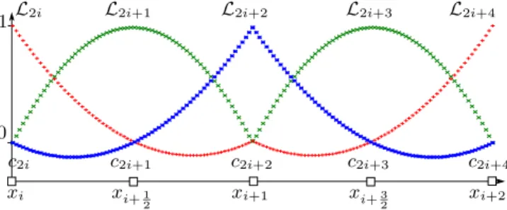
building a uniform Q2 approximation comes to take into account every point (resp. one point over two) of the initial discretization when considering level of resolution j = n (resp. j = n − 1). But using a uniform base (figure 1) leads to errors where function f presents locally strong variations. To keep a good approximation on the whole domain, the finest resolution has to be kept, setting the compression ratio to one.
L2i L2i+1 L2i+2 L2i+3 L2i+4
c2i c2i+1 c2i+2 c2i+3 c2i+4
xi xi+1 2 xi+1 xi+ 3 2 xi+2 1 0
Figure 1: Uniform basis
Instead, we can build a hierarchical base [18]. Let’s build this base by considering only two levels of refinement. Each sub-interval Ij
i can be hierarchically refined by adding two
new basis functions to the existing ones. Then, we define L2i+1 2 by 8 > > > < > > > : L2i+1 2 ∈ P 2([x i, xi+1 2]), L2i+1 2 = 0, if x /∈ [xi, xi+ 1 2], L2i+1 2(xi) = L2i+ 1 2(xi+ 1 2) = 0, L2i+1 2(xi+ 1 4) = 1. (10)
The other basis function L2i+3
2 is defined in the same
man-ner on the interval [xi+1
2, xi+1] (see Figure 2). As we have
added two basis functions for each existing interval, the dimension of the enriched vector space, called ˜Vh, is then
4N + 1 and the approximation ˜fhof f in ˜Vhis given by:
˜ fh(x) = 2N X i=0 ciLi(x) | {z } fh(x) + 2N−1 X i=0 diLi+1 2(x) | {z } gh(x) . (11)
The computation of the coefficients di(often called details)
values (with 0 6 i 6 j): d2i= f (xi+1 4) − 3 8f (xi) − 3 4f (xi+1 2) + 1 8f (xi+1), (12) d2i+1= f (xi+3 4) + 1 8f (xi) − 3 4f (xi+1 2) − 3 8f (xi+1).(13) Considering element [xi, xi+1], Equation (11) can be
evalu-ated at point c = xi+1
4. Then this filter can be easily derived
by using relation (7), the definition of basis functions (10) and the uniform discretization property.
L2i L2i+1 L2i+1 L2i+2
2 L2i+
3 2
c2i d2i c2i+1 d2i+1 c2i+2
xi xi+1 4 xi+ 1 2 xi+ 3 4 xi+1 1 0
Figure 2: Hierarchical basis
Thanks to this hierarchical base (11), the approximation is now splitted into a coarse approximation fh and a
comple-ment noted gh. Considering a function f , function fh can
locally be accurate, leaving ghclose to zero. It implies small
|di| values that can be discarded by the compression
algo-rithm without significant loss of accuracy.
This two levels decomposition can be generalized to a multi-levels decomposition. So we consider a coarse representation at a given level l (with 0 6 l 6 n − 1) and a hierarchical representation from level l to n. We have now a multi-levels decomposition formula f (x) = 2l+1 X i=0 cliL l i(x) + n−1 X j=l 2j X i=0 djiL j i+1 2 (x). (14)
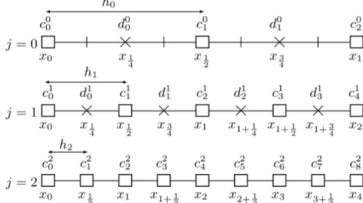
Figure 3 shows a discretization with 9 points (N = 8) and how the hierarchical finite elements framework is mapped on it for a coarse level l = 0.
3.2
Compression Algorithm
The idea of the compression is to compute the different de-tails di(projection of f onto ˜Vhspace) and to keep every cji
coefficient where |dj
i| > ε, with ε a given threshold. In
prac-tice, it comes to discard some values of the function which could be reconstructed with an acceptable error.
So the compression algorithm starts from the level of resolu-tion j = n − 1 and, for each coarser level until a given level l (with 0 6 l 6 n − 1 and 0 6 i 6 2l), the algorithm
com-putes the coefficients dj2iand dj2i+1thanks to Equations (12) and (13). Then, by keeping only |dji| > ε, we build a
com-pressed function fcwith a general wavelet representation:
f (x) ≃ fc(x) = 2l X i=0 cliL l i(x) + n−1 X j=l+1 X |dji|>ε djiL j i+1 2 (x). (15) x0 x0 x0 x1 x1 x1 x2 x2 x3 x4 x1 2 x1 2 x1 2 x1+1 2 x1+1 2 x2+1 2 x3+ 1 2 x1 4 x1 4 x1+1 4 x3 4 x3 4 x1+3 4 j = 0 j = 1 j = 2 h0 h1 h2 c0 0 c01 c02 c1 0 c11 c12 c13 c14 c2 0 c21 c22 c23 c42 c25 c26 c27 c28 d0 0 d01 d1 0 d11 d12 d13
Figure 3: Domain decomposition according to reso-lution levels j (with n = 3)
The calculation of the contribution of dji coefficients can
lead to large computational efforts. The reduction of this cost motivates the approach in [17] which get out of wavelet representation. Instead, we propose to reduce this cost and stay within the wavelet framework by keeping a particular set of coefficients cj
i such that
dJ
i < ε, ∀J > j.
As a consequence, the compressed function fc, built thanks
to Algorithm 1, is given by:
f (x) ≃ fc(x) = X cji∈fc cjiL j i(x). (16)
Input: Discretized function f , compression threshold ǫ Output: Compressed function fc
fc= ∅
for j = n − 1 to j > l step −1 do for i = 0 to i 6 2j− 1 step +1 do
insert= 0 for k = 0, 1 do
Compute dj2i+kapplying eq. (12),(13) if |dj2i+k| > ǫ then
Add I2i+kj+1 to fc
insert= 1 end
end
if insert then Add Ij i to fc
end end
Algorithm 1: Compression algorithm
At the beginning of Algorithm 1, the compressed function fcis empty. For each level of resolution, each element Iij is
considered to compute details dj
2i+k (for k = 0, 1)
belong-ing to this element. When a detail dj2i+k is greater than the threshold ε, all the coefficients belonging to the sub-element I2i+kj+1 are inserted in fc. It consists in inserting the
three coefficients cj+12(2i+k)+lfor l = 0, 1, 2. Note that, for tree structure purpose, if an element of level j + 1 is inserted in fc, his father Iij on level j must be inserted. It means that
The 1D compression algorithm can easily be extended to d dimensions by using a tensor product of 1D transformations. A base of the d-dimensional space is built with all possible products of 1-dimensional basis functions. The main differ-ence in the algorithm is the way elements are considered. In the general d-dimensional case, index i becomes a vector i = (i1, i2, . . . , id) and an element Iijis defined by
Ij i = d Y p=1 Ij ip, (17)
and contains 2d sub-intervals Ij+1
2i+k, k ∈ [0..1] d.
3.3
Simulation Post-processing
Simulation post-processing or visualization pre-processing can be a big issue when dealing with large datasets. When simulation and visualization are considered separately, sev-eral reads/writes of the entire dataset are required, leading to high IO cost. Thus, the integration of our compression scheme into the simulation reduces the IO cost of the simu-lation and suppress completely the post-processing step.
For parallel simulations, this integration is not trivial. But, using our method, the compression of elements Ij
i is
inde-pendent for a same level of resolution j. Thus, only one point on the boundary has to be shared between two ele-ments. Consequently, except a communication step needed to share the boundaries, the compression process and the disk export of the compressed function can be distributed among parallel nodes. This compression scheme has been successfully integrated into our 4D parallel simulation [5, 8] and scales linearly with the number of processors.
4.
4D FUNCTION VISUALIZATION
4.1
Multidimensional Visualization Method
We have adapted the classical hyper-slicing technique de-scribed in [16] to address the 4D volume dataset visualiza-tion issue. This method represents a d−dimensional func-tion with a d × d matrix of views. Each view can be a simple 1D curve plot or a 2D color map plot and displays a particu-lar slice defined by a single focus point P = (p1, p2, . . . , pd).The coordinates of the focus point are displayed and can be modified on each slice. By dragging it in the different views, the user modifies the displayed slices and has the feeling to explore the space as the slices refresh.
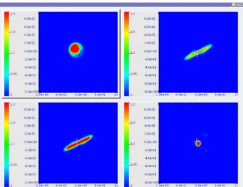
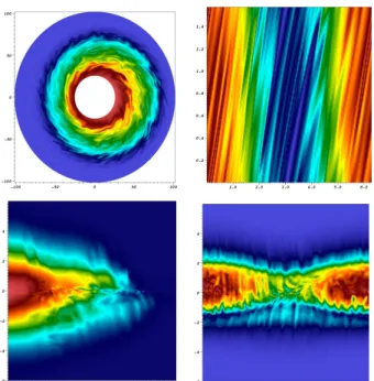
Figure 4 shows a screenshot of our application with a parti-cle beam dataset. Instead of a matrix of views, only four 2D slices are displayed because for this application, the other slices don’t make sense from a physical point of view. Details on the physic can be found in Section 5. Accord-ing to notation (1), the top left view displays the 2D slice Sx,y= f (x, y, pvx, pvy).
Then, refreshing slices at interactive framerates is the crit-ical point of this method. It has been overcome thanks to an efficient (both in storage and random accesses) sparse data structure (section 4.2) and thanks to an efficient slice reconstruction algorithm (section 4.3).
4.2
Data Structure
Figure 4: 4D distribution function from a particle beam simulation. From top to bottom and from left to right are presented the (x, y), (x, vx), (y, vy) and
(vx, vy) slices
The memory representation of fc is not trivial as it is not
a regular array anymore. This mathematical object can be considered as a non structured mesh, composed of a set of elements, each element being a set of points. This approach leads to a point-connectivity representation which is very memory consuming in 4D (1 point = 4 indices and 1 element = 34= 81 points).
Instead, we consider fcas a cloud of points with implicit
re-lations between them. To achieve efficient random accesses, we have designed a dedicated sparse data structure which considers two levels of refinement: one coarse and one fine. All points of a level of resolution j (0 6 j 6 l < n) are stored in the coarse level noted C. As these points are sim-ply an undersampling of the initial discretization, we use a regular 4D array to store fc values. All other points belong
to the fine level and are stored in cells according to their position. Each cell can be seen as a brick that fills the space between points of the coarse level. Figure 5(a) shows, for the 2D case, a partitioned domain with finite elements. Fig-ure 5(b) presents only the points that match elements. It is a cloud of points representation which put them into two classes: coarse grid (disks) or fine cells (crosses). Figure 5(c) presents the memory representation. The coarse grid C is a regular array and fine cells are allocated to store all the other points. A reference to the allocated fine cells is kept in the regular array F .
∅ F C
Cell reference Fine level point
Coarse level point
Figure 5: Sparse data structure
mem-ory when a cell is empty. Otherwise, two types of cell are used: dense and sparse cells. In dense cells, fc values
are stored in regular 4D arrays. They provide random ac-cess in O(1) (one indirection), but are clearly not optimal in memory when they contain only few points. In this case, a lexicographical sorted array of points is used, a point being four integer indices plus the fc value. Thanks to the
sort-ing, such sparse cells provide a O(log(M )) random accesses (with M the number of points in the cell). Consequently, it is possible to optimize the memory consumption by using the appropriate cell type according to the bag-filling ratio of the cell. For example, in four dimensions with four bytes integer indices and four bytes floating point function value, it is cheaper to use a sparse cell when the filling ratio is lower than 50%, and a dense cell otherwise.
To sum up, this data structure can be seen as a dedicated hashmap implementation. Point indices play the role of the key which is associated to the fc value. The hash
func-tion is a trivial shifting/masking operafunc-tion. By optimizing its memory consumption, we are able to load completely the whole compressed function into the core memory. By keeping efficient random accesses, we ensure the interactive performances of the reconstruction algorithm.
4.3
Reconstruction Process
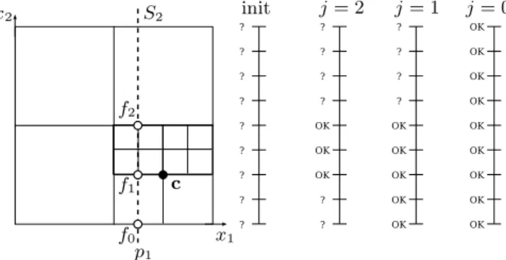
The slice reconstruction algorithm uses the finite element property saying that whatever the point considered inside an element, the value of the function at this point can be built with the function value on this element. So, the principle of the algorithm consists in computing the intersection between the 2D slice and the different 4D elements. Then the value of the function is computed on the 2D slice on the finest level of resolution in order to build the displayed colormap.
Input: Focus point p, 2D compressed function fc
Output: Slice S2 Set S2 to undefined ; for j = n − 1 to j > l step j -= 1 do hj= 2n−jh; c = ⌊p/hj⌋hj+ hj/2; for c2= hj/2 to c262nstep c2 +=hj do if fc(c) exists then m = c2− hj/2; M = c2+ hj/2; L = BuildPolynomial(fc, j, c, p); for x2= m to x26M step x2 +=h do
if S2(x2) is not defined then
S2(x2) = L “2(x 2−m) M−m ” ; end end end end end
Algorithm 2: Slice extraction
The data structure described in previous section does not store explicitly element information. But it exists implicitly because, thanks to the compression algorithm, every point required for it are present in fc. And a sufficient condition
to know if element Iij exists, is the presence of its center
c f0 f1 f2 p1 S2 init j = 2 j = 1 j = 0 x1 x2
Figure 6: 1D slice extraction from a 2D function
C(Iij) defined by
C(Iij) =xi+ xi+1 2 = xi+
hj
2. (18) We can show that this point belongs only to element Ij
i when
considering level of resolution j. For the sake of simplicity, Algorithm 2 presents the extraction of the 1D slice S2(x2)
from a 2D compressed function fc(x), with x = (x1, x2) and
for the focus point p = (p1, p2).
At the beginning, all points of the slice are undefined. Then for each level of resolution j, centers c = (c1, c2) of all
possi-ble intersecting elements are computed. Once an intersect-ing element is found (presence of its center in fc), the 1D
Lagrange polynomial L is built. Its construction is described below. This polynomial is the approximation of f on the in-tersection between the slice and the domain of f : interval [c2− hj/2, c2+ hj/2]. Then it is evaluated to build, on the
whole intersection area, a discretization of the function at the finest level of resolution (step h). But values are actually written in the slice only at positions that are still undefined. If a value is already defined in the slice, it means that it has been computed using a finer level of resolution, i.e. with a better accuracy. Figure 6 presents the state of the slice for different levels j during Algorithm 2.
Thanks to tensor product construction of the 2D base, the approximation of function f on interval [c2−hj/2, c2+hj/2]
is a 1D Lagrange polynomial. By considering the reference element [0, 2], we build the reference polynomial L
L(x) = f0+ (f1− f0)x +1
2(f2− 2f1+ f0)x(x − 1), (19) with f0 = fc(p1, c2 − hj/2), f1 = fc(p1, c2) and f2 =
fc(p1, c2+ hj/2). But these three values may not exist in
fc. In this case, they have to be built by using a similar
1D polynomial, but in the other dimension. For example, on figure 6, while considering center c at level j = 1, the f0
value doesn’t exist in fc. So the 1D Lagrange polynomial
L0 is built using fc(c1− hj/2, c2 − hj/2), fc(c1, c2− hj/2)
and fc(c1+ hj/2, c2− hj/2) and is evaluated at point p1 to
know f0.
If we note M the number of points in the slice, the com-plexity of this algorithm is in O(M ). As the amount of computations is not very important, the execution fastness depends on the random accesses efficiency to fcvalues.
compressed function fc(x1, x2, x3, x4) is almost the same.
Now the traversal of the possible intersecting elements is a 2D traversal. In the same manner, the traversal which fills the slice with the function value is also a 2D traversal. Finally, the polynomial computation can be performed by several 1D interpolations as in 2D.
5.
RESULTS
We mainly apply our technique to the interactive exploration of plasmas behavior. Plasma can be considered as the fourth state of material, which appears for huge temperature and pressure conditions (104K or more). These conditions are
reached in different facilities, like fusion reactors (tokamak) and particle beam accelerators. Plasma is then modelled by a time-varying particle distribution function which lives in phase space, the product of the physical space with the ve-locities space. A Cartesian frame is used for particle beam and laser-material interaction. The 2D physical space (x, y) with the 2D velocities space (vx, vy) lead to a 4D distribution
function f (x, y, vx, vy). Numerical methods [5, 8] compute
such 4D functions and integrate our compression scheme. Figure 4 (resp. 9) presents the visual result and figure 7 (resp. 8) presents the performances of our method for a par-ticle beam (resp. plasma) simulation.
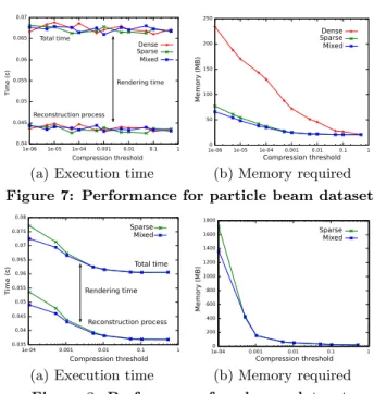
(a) Execution time (b) Memory required Figure 7: Performance for particle beam dataset
(a) Execution time (b) Memory required Figure 8: Performance for plasma dataset The different tests are performed within a single thread on an Intel Pentium D (3.4 GHz, 2 MB cache). The evaluation of the visualization performances is carried out with a 2564 grid, which represents 32GB array of double precision float. Three data structures that use different types of cells (cf Section 4.2) are compared. The “dense” test uses only dense cells, the “sparse” test, only sparse cells and the “mixed” test contains both types in order to optimize the memory consumption. Even with a good data size reduction, the required memory for plasma data is too large, this is the reason why we studied performances only for sparse and mixed data structure and only until threshold ε = 10−4.
Figure 7(a) and 8(a) show the execution time of the visualization loop (focus point modification slice computation
-Figure 9: 4D function from plasma simulation. From top to bottom and from left to right are presented the (x, y), (x, vx), (y, vy) and (vx, vy) slices
rendering) according to the compression threshold ε. As the displayed slices are always the same size, the rendering time is always the same (≃ 25ms). The interactive frame rate of 10 fps is reached whatever the threshold and the type of cell. The increase of the execution time for low thresholds on Figure 8(a) comes from the large number of elements in the sparse data structure and its size leading to poor cache reuse. Figure 7(b) and 8(b) show the amount of memory re-quired to load the entire compressed function into the core memory according to the compression threshold ε. As we ex-pect, the mixed data structure presents the lowest memory consumption.
To sum up, according to a reasonable compression thresh-old ε = 10−3, this compression scheme enables to reduce the data size by two orders of magnitude. And the sparse data structure provides random accesses efficient enough to make the reconstruction process interactive, giving to the user the illusion of the 4D exploration. So we can visualize 4D functions hundred times bigger with the same computer or visualize the same function on a computer hundred times smaller.
This technique has been recently implemented in the 5D non-linear GYrokinetic SEmi-LAgrangian code (GYSELA). This code is developed at CEA Cadarache to perform simu-lations of ion turbulence in tokamak plasmas. Understand-ing turbulent transport in magnetized plasma is a subject of outmost importance for comprehending and optimizing ex-periments in the present fusion devices and also for designing future reactors. The development of such a 5D code (3D in real toroidal space (r, θ, ϕ) and 2D in velocity space (the par-allel velocity vk+ the magnetic momentum µ) is extremely
challenging not only in terms of CPU time consumption and available memory size but also in terms of visualization. In-deed, one actual typical 5D distribution function needs 64 GB memory. Until now, only few 2D slices of this distribu-tion funcdistribu-tion were exploited, typically poloidal cross-secdistribu-tions Sr,θ for two or three focus points. Now, this tool provides
Figure 10: 4D function from gyrokinetic simulation. From top to bottom and from left to right are pre-sented the (r, θ), (θ, ϕ), (r, vk) and (θ, vk) slices
the performances of the simulation code. Figure 10 shows a 4D distribution function f (r, θ, ϕ, vk) obtained by setting
a specific µ in the 5D function. In particular, we notice on slice (θ, vk) the filamentation which appear in vk direction
in a developping turbulence phase.
6.
CONCLUSIONS AND FUTURE WORK
This paper presents a multidimensional visualization method for the exploration of 4D scalar fields. Its main con-tribution is the design of a dedicated compression scheme that both reduces significantly the size of the data and can be easily integrated into parallel simulation codes. The sparse data structure gives an efficient memory representa-tion to store the compressed funcrepresenta-tion and provides random accesses efficient enough to make the reconstruction process interactive. Finally, we provide an efficient tool for physi-cists which allows them to explore their data.This work can be improved in both mathematical and computer science ways. Anisotropic compression scheme could allow good compression ratios even for functions which present strong variations over the whole domain. In-deed, compression ratio has to be improved for gyrokinetic datasets. An out-of-core extension can be designed thanks to the multiresolution representation of the data. These extensions would allow the visualization of even bigger 4D functions.
7.
ACKNOWLEDGMENTS
This work has been done at LSIIT lab (Illkirch, France) and funded by Alsace Region, IRMA lab and INRIA. Thanks to Virginie Grandgirard from CEA Cadarache (France) and Eric Sonnendrucker from IRMA lab (Strasbourg, France) for gyrokinetic and particle beam datasets and feed back on the visualization tool.
8.
REFERENCES
[1] D. Asimov. The grand tour: a tool for viewing multidimensional data. SIAM J. Sci. Stat. Comput., 6(1):128–143, 1985.
[2] C. Bajaj, I. Ihm, and S. Park. 3d rgb image compression for interactive applications. ACM Trans. Graph., 20(1):10–38, 2001.
[3] C. Bajaj and V. Pascucci. Hypervolume visualization: A challenge in simplicity. Technical report, Austin, TX, USA, 1998.
[4] P. G. Ciarlet and J.-L. Lions, editors. Handbook of numerical analysis. Vol. II. North-Holland, 1991. [5] N. Crouseilles, G. Latu, and E. Sonnendr¨ucker. Hermite
spline interpolation on patches for parallel Vlasov beam simulations. Nuclear Instruments and Methods in Physics Research A, 577:129–132, July 2007.
[6] S. R. dos Santos and K. W. Brodlie. Visualizing and investigating multidimensional functions. In Symposium on Data Visualisation (VISSYM’02), pages 173–182,
Aire-la-Ville, Switzerland, 2002. Eurographics Association. [7] N. Fout, K.-L. Ma, and J. Ahrens. Time-varying,
multivariate volume data reduction. In ACM symposium on Applied computing (SAC’05), pages 1224–1230, New York, NY, USA, 2005. ACM Press.
[8] V. Grandgirard, Y. Sarazin, P. Angelino, A. Bottino, N. Crouseilles, G. Darmet, G. Dif-Pradalier, X. Garbet, P. Ghendrih, S. Jolliet, G. Latu, and E. Sonnendr¨ucker. Global full-f gyrokinetic simulations of plasma turbulence. Plasma Phys. Control. Fusion, 49:B173–B182, 2007. [9] M. H. Gross, L. Lippert, and O. G. Staadt. Compression
methods for visualization. Future Gener. Comput. Syst., 15(1):11–29, 1999.
[10] S. Guthe and W. Straßer. Real-time decompression and visualization of animated volume data. In Conference on Visualization (VIS’01), pages 349–356, Washington, DC, USA, 2001. IEEE Computer Society.
[11] P. Hoffman and G. Grinstein. A survey of visualizations for high-dimensional data mining. Information visualization in data mining and knowledge discovery, pages 47–82, 2002. [12] I. Ihm and S. Park. Wavelet-based 3D compression scheme
for very large volume data. In Graphics Interface, pages 107–116, 1998.
[13] L. Linsen, V. Pascucci, M. A. Duchaineau, B. Hamann, and K. I. Joy. Hierarchical representation of time-varying volume data with ”4th-root-of-2” subdivision and quadrilinear b-spline wavelets. In Conference Pacific Graphics, page 346, Washington, DC, USA, 2002. IEEE Computer Society.
[14] N. Neophytou and K. Mueller. Space-time points: 4d splatting on efficient grids. In IEEE symposium on Volume visualization and graphics (VVS’02), pages 97–106, Piscataway, NJ, USA, 2002. IEEE Press.
[15] H.-W. Shen, L.-J. Chiang, and K.-L. Ma. A fast volume rendering algorithm for time-varying fields using a time-space partitioning (tsp) tree. In Conference on Visualization (VIS’99), pages 371–377, Los Alamitos, CA, USA, 1999. IEEE Computer Society Press.
[16] J. van Wijk and R. van Liere. Hyperslice: visualization of scalar functions of many variables. In Conference on Visualization (VIS’93), pages 119–125, 1993.
[17] J. Wilhelms and A. V. Gelder. Multi-dimensional trees for controlled volume rendering and compression. In
Symposium on Volume visualization (VVS’94), pages 27–34, New York, NY, USA, 1994. ACM Press.
[18] H. Yserentant. Hierarchical bases. In O’Malley and R. E., editors, ICIAM 91, pages 256–276, Washington, DC, 1992. SIAM, Philadelphia.
[19] J. Ziv and A. Lempel. A universal algorithm for sequential data compression. IEEE Trans. Inf. Theory, 23(3):337–343, 1977.