HAL Id: tel-03185160
https://tel.archives-ouvertes.fr/tel-03185160
Submitted on 30 Mar 2021HAL is a multi-disciplinary open access archive for the deposit and dissemination of sci-entific research documents, whether they are pub-lished or not. The documents may come from teaching and research institutions in France or
L’archive ouverte pluridisciplinaire HAL, est destinée au dépôt et à la diffusion de documents scientifiques de niveau recherche, publiés ou non, émanant des établissements d’enseignement et de recherche français ou étrangers, des laboratoires
with tree tensor networks for Uncertainty Quantification
Cecile Haberstich
To cite this version:
Cecile Haberstich. Adaptive approximation of high-dimensional functions with tree tensor networks for Uncertainty Quantification. Data Structures and Algorithms [cs.DS]. École centrale de Nantes, 2020. English. �NNT : 2020ECDN0045�. �tel-03185160�
Je souhaite tout d’abord remercier les membres de mon jury. Merci à Fabio Nobile et Lars Grasedyck pour leur relecture approfondie du manuscrit ainsi que leurs questions lors de la soute-nance qui témoignent de leur intérêt pour ces travaux de thèse. First of all, I would like to thank the jury’s members. Fabio Nobile and Lars Grasedyck, thank you, for your thorough reviewing of the manuscript as well as your questions during the defense, which show your interest in this work. Merci à Albert Cohen pour avoir présidé ce jury et merci à Virginie Ehrlacher pour sa présence enthousiaste et son intérêt.
Anthony et Guillaume merci infiniment. Merci à tous les deux pour votre engagement et votre enthousiasme pour cette thèse, sans oublier votre bienveillance durant ces trois années.
Introduction 8
1 Projection methods 29
1.1 Introduction . . . 29
1.2 Interpolation . . . 29
1.2.1 Interpolation in the one-dimensional case . . . 31
1.2.2 Interpolation with any arbitrary approximation space . . . 33
1.2.3 Interpolation with tensor product bases . . . 34
1.3 Least-squares method . . . 35
1.3.1 Weighted least-squares projection . . . 36
1.3.2 Random sampling . . . 38
1.3.3 Optimal sampling measure . . . 40
2 Boosted Optimal Weighted Least-Squares 43 2.1 Introduction . . . 43
2.2 Boosted optimal weighted least-squares method . . . 44
2.2.1 Resampling and conditioning . . . 45
2.2.2 Subsampling . . . 49
2.3 The noisy case . . . 51
2.4 Numerical experiments . . . 54
2.4.1 Notations and objectives . . . 54
2.4.2 Qualitative analysis of the boosted optimal weighted least-squares method . . 56
2.4.3 Quantitative analysis for polynomial approximations . . . 59
2.4.4 A noisy example . . . 68
2.4.5 Overall conclusion for all examples . . . 69
2.5 Conclusion . . . 70
3 Adaptive Boosted Optimal Weighted Least-Squares 75 3.1 Introduction . . . 75
3.2 Notations . . . 76
3.3 Optimal weighted least-squares with block-structured sampling . . . 77
3.3.2 Adaptive approximation with a nested sequence of spaces . . . 78
3.4 Boosted optimal weighted least-squares with block-structured sampling . . . 79
3.4.1 Approximation in a given space . . . 79
3.4.2 Adaptive approximation with a nested sequence of spaces . . . 83
3.5 Numerical illustrations . . . 85
3.5.1 Illustration of the stability of the adaptive boosted least-squares strategy . . 85
3.5.2 Illustration for polynomial approximation . . . 89
3.6 Conclusion . . . 92
4 Tree-based tensor formats 95 4.1 Introduction . . . 95
4.2 Tensor spaces . . . 95
4.3 Tensor ranks and tree-based tensor formats . . . 96
4.3.1 Dimension partition tree . . . 97
4.3.2 Tree tensor networks and their representation . . . 98
4.4 Principal Component Analysis for multivariate functions . . . 101
4.4.1 α-principal subspaces . . . 101
4.4.2 Accuracy of the empirical α-principal subspaces . . . 102
4.4.3 The case of functions with Sobolev regularity . . . 103
4.5 Approximation power of tree tensor networks . . . 105
4.5.1 Truncation in tree-based format . . . 105
4.5.2 Approximation rates for Sobolev functions . . . 106
5 Principal Component Analysis for Tree-based tensor formats 107 5.1 Approximation of α-principal subspaces . . . 108
5.1.1 Choosing an oblique projection verifying a stability property . . . 108
5.1.2 Choosing the boosted optimal weighted least-squares projection . . . 110
5.2 Estimation of the α-principal subspaces . . . 113
5.2.1 Accuracy of the empirical α-principal subspaces . . . 113
5.2.2 Adaptive estimation of the α-principal component subspaces . . . 116
5.3 Learning tree tensor networks using PCA . . . 117
5.3.1 Description of the algorithm . . . 117
5.3.2 Error analysis . . . 118
5.3.3 Complexity analysis . . . 121
5.3.4 Heuristics used in practice . . . 122
5.4 Numerical examples . . . 124
5.4.1 Notations and objectives . . . 124
5.4.3 Adaptive estimation of the α-principal components subspaces . . . 126
5.5 Conclusions . . . 130
6 Tree adaptation 137 6.1 Introduction . . . 137
6.2 Estimation of α-ranks . . . 139
6.2.1 Principle and algorithm . . . 139
6.2.2 Numerical illustration . . . 141
6.3 Leaves-to-root construction of the tree with local deterministic optimizations . . . . 143
6.3.1 Max-mean rank strategy . . . 143
6.3.2 Ballani and Grasedyck’s strategy . . . 145
6.4 Leaves-to-root construction of the tree with local stochastic optimizations . . . 146
6.4.1 Principle and algorithm . . . 146
6.4.2 Illustration of the algorithm . . . 147
6.4.3 Illustration of the choices of the parameters . . . 147
6.5 Adaptation of the tree with global stochastic optimizations . . . 150
6.5.1 Principle and algorithm . . . 150
6.5.2 Illustration of the algorithm . . . 150
6.5.3 Illustration of the choice of the parameters . . . 151
6.6 Numerical examples . . . 153
6.7 Conclusions . . . 157
Conclusion 159 A Approximate fast greedy algorithm 172 A.1 Computational strategy for the approximate fast greedy algorithm . . . 172
A.2 Complexity analysis . . . 173
A.3 Illustration . . . 174
B Sampling of multivariate probability distribution in Tree-Based tensor formats177 B.1 Probability distributions in tree-based format . . . 177
B.1.1 Marginal distributions . . . 178
B.1.2 Conditional distributions . . . 179
Contexte
Grâce à des modèles de calcul, les chercheurs et les ingénieurs peuvent remplacer des expéri-ences physiques particulièrement coûteuses et complexes à mettre en œuvre par des simulations numériques. La réponse d’un modèle dépendant de certains paramètres peut être représentée par une fonction u(x1, . . . , xd) de plusieurs variables. Malgré l’amélioration continue des ressources de
calcul, la plupart de ces simulations restent très coûteuses d’un point de vue informatique. En outre, la résolution des problèmes de quantification de l’incertitude (UQ), comprenant notamment la propagation des incertitudes, la calibration des modèles, les problèmes inverses ou l’analyse de sensibilité [87], nécessite un grand nombre d’évaluations des modèles. Une solution consiste alors à remplacer le modèle coûteux par un modèle approché, moins coûteux à évaluer, ce qui revient à remplacer la fonction qui représente la réponse du modèle par une approximation.
Le but de l’approximation est de remplacer une fonction u par une fonction plus simple (c’est-à-dire plus facile à évaluer) de telle sorte que la distance (mesurant la qualité de l’approximation) entre la fonction u et son approximation, notée u⋆, soit aussi petite que possible. En général,
l’approximation est recherchée dans un sous-espace de fonctions Vm décrit par un certain nombre
de paramètres m. Une séquence de tels sous-espaces (Vm)m≥1 est appelée outil d’approximation
(ou classe de modèles), dont la complexité est mesurée par son nombre de paramètres m. L’erreur de meilleure approximation de u par des éléments de Vm est définie par la distance minimale entre
u et tout élément de Vm. L’outil d’approximation doit être adapté à la classe de fonctions que nous
voulons approximer, ce qui se traduit par une erreur de meilleure approximation qui converge vers zéro assez rapidement avec m.
Il existe différentes approches pour construire l’approximation d’une fonction, soit à partir d’informations directes sur la fonction (par exemple des évaluations ponctuelles ou des mesures linéaires...), soit à partir d’équations satisfaites par la fonction. Dans cette thèse, nous nous intéres-sons aux fonctions de type boîte noire (éventuellement bruitées), ce qui correspond à la première situation où l’information sur u est donnée par des échantillons. Par conséquent, pour constru-ire l’approximation de la fonction u, nous utilisons les évaluations yi = u(xi) pour un ensemble
de points xi ou yi = u(xi) + ei dans le cas de données bruitées. Cependant, dans le contexte
d’échantillons, idéalement proche du nombre de paramètres m. Les échantillons xi peuvent être
soit indépendants et identiquement distribués selon une mesure µ, soit sélectionnés de manière adaptative. Cette seconde approche est particulièrement pertinente lorsqu’aucune évaluation de la fonction n’a encore été faite, ce qui sera le cadre de cette thèse.
Des méthodes typiques pour construire une approximation à partir d’échantillons sont l’interpolation et les méthodes des moindres carrés [28]. Les méthodes d’interpolation classiques comprennent l’interpolation polynomiale et l’interpolation par spline (où les échantillons sont en général choisis par rapport à Vm, pour garantir de bonnes propriétés des opérateurs d’interpolation), ainsi que le
krigeage (qui est assez efficace lorsque les échantillons sont donnés et peut être amélioré avec une sélection adaptative des échantillons) [82]. Pour un ensemble de m points, x1, . . . , xml’interpolation
u⋆ de u dans V
m est définie par
u(xi) = u⋆(xi), pour tout 1 ≤ i ≤ m.
L’interpolation est bien étudiée dans le cas unidimensionnel mais dans le cas multivarié (d > 1), trouver de bons points pour l’interpolation est un problème difficile, en particulier lorsque Vm est
un espace d’approximation non classique. En pratique, [18, 19] proposent des stratégies pour con-struire de bonnes séquences de points pour l’interpolation parcimonieuse utilisant des polynômes ou splines tensorisés. Cependant, pour les espaces d’approximation non classiques, même si certains ensembles de points ont montré leur efficacité (voir [65, 15]), il n’y a pas de garantie pour l’erreur d’interpolation.
Pour n échantillons x1, . . . , xnindépendants et identiquement distribués selon une mesure µ, la
méthode des moindres carrés classique définit l’approximation de u comme le minimiseur de
min v∈Vm 1 n n X i=1 (v(xi) − yi)2.
Un aspect intéressant des méthodes des moindres carrés est qu’elles sont capables, sous certaines conditions sur le nombre d’échantillons n, de garantir une approximation stable et une erreur proche de l’erreur de meilleure approximation mesurée avec la norme L2
µ. Toutefois, pour ce faire, elles
peuvent exiger une taille d’échantillon n bien supérieure à m (voir [22]). Les méthodes des moin-dres carrés sont un cas particulier de minimisation de risque empirique en apprentissage supervisé [30]. D’autres fonctionnelles de risque peuvent être utilisées, mais elles nécessitent également de nombreuses évaluations afin d’assurer la stabilité.
d’estimation peut être améliorée en utilisant les moindres carrés pondérés [32, 73], qui définit l’approximation de u par min v∈Vm 1 n n X i=1 wi(v(xei) − yi)2,
où les poids sont adaptés à Vm et les pointsxei sont des échantillons indépendants et identiquement
distribués selon une mesure bien choisie. Cela peut permettre de réduire la taille de l’échantillon n pour atteindre la même erreur d’approximation, par rapport aux moindres carrés standards. Dans [24], les auteurs introduisent une mesure d’échantillonnage optimale dont la densité par rapport à la mesure de référence dépend de l’espace d’approximation Vm. Ils montrent que la projection des
moindres carrés pondérés construite avec des échantillons de cette mesure est stable en espérance avec des valeurs de n plus faibles qu’avec les moindres carrés classiques. Une approche similaire est proposée dans [68], où la principale différence est que les échantillons aléatoires sont plus structurés tout en garantissant des résultats de stabilité similaires. Néanmoins, dans les deux cas, la condition nécessaire pour avoir une stabilité exige toujours un nombre élevé d’échantillons n, par rapport à une méthode d’interpolation. Les auteurs proposent également des méthodes de moindres carrés pondérés optimales dans le cas d’une approximation adaptative (lorsque Vm est choisi dans une
séquence d’espaces d’approximation imbriqués), voir [67] et [4]. Dans cette thèse, nous proposons une nouvelle méthode de projection sur un espace d’approximation fixe Vm qui assure la stabilité
de la projection des moindres carrés en espérance avec une taille d’échantillon proche de m. Nous proposons également une nouvelle méthode pour le cadre adaptatif qui réduit de manière significa-tive le nombre d’échantillons et présente toujours des propriétés de stabilité.
Dans de nombreuses applications, les fonctions peuvent dépendre d’un nombre potentiellement élevé de variables d ≫ 1. Lorsque la dimension d augmente, l’utilisation d’outils d’approximation standards adaptés aux fonctions régulières (par exemple les splines pour les fonctions de Sobolev) conduit à une complexité des méthodes d’approximation qui croît de manière exponentielle avec d. C’est ce qu’on appelle la malédiction de la dimension, expression introduite par [12]. Par conséquent, le nombre d’évaluations nécessaires pour approcher la fonction u avec des outils d’approximation naïfs peut exploser. Dans cette thèse, nous supposons que les fonctions présen-tent des structures de faible dimension, de sorte que nous pouvons nous attendre à une bonne approximation en utilisant un nombre limité d’évaluations de la fonction. L’exploitation de ces structures de la fonction nécessite généralement des outils d’approximation particuliers [29], qui peuvent dépendre de l’application. Certains outils d’approximation parmi les plus courant sont rappelés ci-après.
Une première approche consiste à utiliser la parcimonie de u en choisissant un ensemble par-ticulier de fonctions {ϕj}j∈Λ parmi un ensemble de fonctions de base tensorisées, de sorte que
u puisse être écrit sous la forme Pj∈Λajϕj(x). Des méthodes d’approximation parcimonieuses
ont été envisagées pour résoudre les problèmes de quantification d’incertitude, voir par exemple [23, 6, 5, 18, 19] pour une approximation polynomiale parcimonieuse.
Des classes de modèles plus structurées pour traiter les problèmes de grande dimension sont les modèles additifs, introduits par [41],Pd
i=juj(xj) ou plus généralementPα∈Tuα(xα) où T ⊂ 2{1,...,d}
est soit fixe (cela correspond à une approximation linéaire), soit un paramètre libre (cela correspond à une approximation non linéaire). Il existe également des modèles multiplicatifs Qdj=1uj(xj) ou
plus généralement Qα∈Tuα(xα), où T est également un sous-ensemble de 2{1,...,d} et la même
dis-tinction entre approximation linéaire et non linéaire est faite, selon que T est fixe ou non. Ces types d’outils d’approximation sont standards en statistique et en modélisation probabiliste (mod-èles graphiques, réseaux bayésiens).
Des classes de modèles plus complexes basées sur la composition des fonctions ont également été proposées. Parmi elles, les modèles ridge peuvent être écrits sous la forme v(W x) avec W ∈ Rk×d,
où v appartient à une classe de fonctions de k variables avec une paramétrisation de faible dimen-sion. Un exemple typique est le perceptron aσ(wTx + b), où σ est une fonction d’activation donnée,
introduit dans [83]. Ces modèles de composition comprennent également le modèle de projection pursuit Pk
j=1vj(wTjx), où pour j = 1, . . . , k, wj ∈ Rd, voir [41, 42]. Un cas particulier est celui
des réseaux de neurones avec une couche cachée Pd
j=1ajσ(wjTx + bj). On peut aussi considérer des
compositions de fonctions plus générales, telles que vL◦vL−1◦. . .◦v1. Dans le cas des réseaux de
neu-rones profonds, pour chaque j = 1, . . . , L, les fonctions vj s’écrivent vj(t) = σ(Ajt+bj), où σ est une
fonction d’activation choisie, tandis que bj ∈ Rk et Aj ∈ Rk×d sont des paramètres à estimer [45].
Malgré son formalisme général et les nombreux succès qu’ils ont acquis en matière d’approximation, les réseaux de neurones profonds nécessitent généralement un nombre élevé d’évaluations pour ap-prendre les paramètres, ce qui n’est pas possible dans le contexte d’évaluations coûteuses. De plus, lorsque l’on considère les fonctions d’activation non linéaires générales, il est difficile de garantir une approximation stable dont l’erreur est proche de l’erreur de meilleure approximation, ce qui est un objectif central de cette thèse.
Dans ce travail, nous nous concentrons sur les modèles de fonctions de faible rang et en partic-ulier sur l’ensemble des fonctions dans les formats de tenseurs basés sur des arbres ou les réseaux de tenseurs basés sur des arbres, qui peuvent être considérés comme une classe particulière de réseaux de neurones. Plus précisément, pour α un sous-ensemble de D = {1, . . . , d} et αc = D \ α son
complémentaire dans D, nous considérons les fonctions qui peuvent être écrites
v(x) = rα X i=1 uαi(xα)uα c i (xαc), for all α ∈ T, (1)
où T est un arbre de partition de dimension. Un arbre de partition de dimension est une collection particulière de sous-ensembles de D, quelques exemples d’arbres sont donnés Figure 1. L’entier minimal rα tel que v peut être écrit sous la forme (1) est appelé le rang α de v, noté rankα(v).
{1, 2, 3, 4, 5} {1} {2} {3} {4} {5} Arbre trivial {1, 2, 3, 4, 5} {1, 2, 3, 4} {1, 2, 3} {1, 2} {1} {2} {3} {4} {5}
Arbre binaire linéaire
{1, 2, 3, 4, 5} {1, 2, 3} {1} {2, 3} {2} {3} {4, 5} {4} {5}
Arbre de partition de dimension quelconque
Figure 1 – Exemples d’arbres de partition de dimension
L’ensemble des fonctions dans un format de tenseurs basé sur des arbres est défini par TT r (H) =
{v ∈ H : rankα(v) ≤ rα, α∈ T }, avec r = (rα)α∈T un tuple d’entiers, et H un espace d’approximation
de fonctions multivariées. Il comprend le format de Tucker pour un arbre trivial, le format tensor-train (tensor-train de tenseurs) pour un arbre binaire linéaire [79] et le format hiérarchique plus général pour un arbre de partition de dimension quelconque [54]. Toute fonction dans TT
r (H) admet une
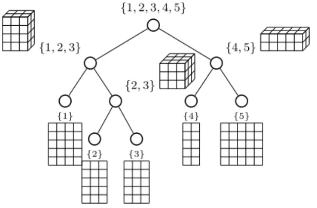
paramétrisation multilinéaire avec des paramètres formant un réseau de tenseurs de faible ordre, d’où le nom de réseaux de tenseurs basés sur des arbres, voir la Figure 2 pour une illustration pour d = 5. Considérer les arbres de dimension pour T donne de bonnes propriétés topologiques et géométriques à l’ensemble TT
r (H) [35, 37]. Les réseaux de tenseurs basés sur des arbres sont
particulièrement pertinents pour l’approximation en grande dimension, car la complexité de la paramétrisation d’une fonction est linéaire en la dimension d et polynomiale en les rangs [53]. Ils peuvent également être utilisés pour l’approximation de fonctions univariées [2, 3]. Toutefois, les rangs (et donc le nombre d’évaluations n) nécessaires pour calculer une approximation dans un format de tenseurs basé sur des arbres avec une tolérance donnée peuvent dépendre fortement de l’arbre choisi T . La classe de modèles TT
r (H) peut également être interprétée comme une classe
de fonctions qui sont des compositions de fonctions multilinéaires, la structure des compositions étant donnée par l’arbre. Elle a été identifiée avec une classe particulière de réseaux de neurones profonds (plus précisément les réseaux somme-produit ou les circuits arithmétiques) avec une con-nectivité parcimonieuse [26]. L’erreur d’approximation associée à cette classe de modèles a deux contributions : l’erreur de troncature (due aux rangs finis r) et l’erreur de discrétisation (due à
{1, 2, 3, 4, 5} {1, 2, 3} {1} {2, 3} {2} {3} {4, 5} {4} {5}
Figure 2 – Un réseau de tenseurs basé sur des arbres admet une paramétrisation multilinéaire avec des paramètres formant un réseau de tenseurs de faible ordre.
l’introduction de l’espace de dimension finie H).
Les réseaux de tenseurs basés sur des arbres sont un outil d’approximation qui permettent d’obtenir de bonnes performances pour de nombreuses classes de fonctions. Dans [84] ou plus récemment dans [7, 2, 3], les auteurs montrent que pour les fonctions u avec une régularité Sobolev, ils atteignent (quel que soit l’arbre) un taux d’approximation optimal ou proche de l’optimal [61]. Ils prouvent également que pour les fonctions u avec une régularité Sobolev mixte, l’approximation dans un format de tenseur basé sur des arbres atteint presque la performance idéale obtenue par une approximation avec croix hyperbolique. Pour une revue de la littérature sur les méthodes d’approximation de faible rang, voir [47]. Nous renvoyons également le lecteur à la monographie [53] et à [8, 36, 59, 60, 77, 76].
Dans la littérature, des algorithmes construisant des approximations dans des formats de tenseurs basés sur des arbres en utilisant des évaluations ponctuelles de fonctions ont déjà été proposés. D’une part, il y a des approches d’apprentissage statistique qui utilisent des évaluations aléatoires et non structurées des fonctions [48, 55]. La robustesse et l’efficacité de ces algorithmes sont démontrées par des expériences numériques, mais ces algorithmes sont principalement basés sur des heuristiques et manquent d’une analyse approfondie. D’autre part, il y a les algorithmes qui utilisent des évaluations adaptatives et structurées des tenseurs, voir [64] (pour le format Tucker), ou [80] et [78] pour les formats de tenseurs basés sur des arbres. Parmi les approches adaptatives, la méthode de [78] présente un intérêt particulier. L’auteur propose une variante de la décomposi-tion en valeurs singulières d’ordre supérieur (HOSVD) (des adaptadécomposi-tions antérieures de la HOSVD ont été faites en [46] et [80]). Le principe consiste à construire une hiérarchie de sous-espaces optimaux qui aboutit à la construction d’un espace produit tensoriel dans lequel la fonction u
est projetée, pour définir l’approximation finale u⋆. En se basant sur des hypothèses fortes sur
l’erreur d’estimation faite dans la détermination des sous-espaces, l’auteur de [78] montre qu’avec un certain nombre d’évaluations de l’ordre de la complexité de stockage du format de tenseurs, l’approximation satisfait l’erreur souhaitée à des constantes près dépendant de certains opérateurs de projection, qui ne sont pas quantifiées.
Toutes ces conclusions montrent que les résultats théoriques sur la convergence des algorithmes existants sont limités. Dans cette thèse, nous proposons un algorithme qui construit une approxi-mation u dans un format de tenseur basé sur des arbres, en utilisant un échantillonnage adaptatif et structuré avec quelques garanties théoriques, et nous proposons des stratégies heuristiques pour obtenir une approximation avec une précision souhaitée et une complexité quasi optimale.
Contributions
Plus précisément, les contributions de cette thèse peuvent être résumées à travers les objectifs suivants :
1. Proposer une méthode de projection dans un espace d’approximation linéaire, basée sur des techniques d’échantillonnage, qui soit stable et dont la construction nécessite un nombre d’évaluations proche de la dimension de l’espace d’approximation.
2. Proposer une stratégie pour construire des projections linéaires sur une séquence d’espaces d’approximation imbriqués, en utilisant un nombre réduit d’échantillons.
3. Proposer une méthode pour construire l’approximation d’une fonction dans un format de tenseur basé sur des arbres, avec des garanties de stabilité théoriques et proposer des heuris-tiques pour contrôler l’erreur.
4. Proposer une stratégie pour choisir l’arbre de dimension T afin de réduire les rangs de l’approximation à une précision donnée et donc sa complexité et le nombre d’évaluations requises.
Cette thèse est divisée en six chapitres. Les chapitres 1 et 4 font le point sur les méthodes de projection sur les espaces d’approximation linéaires et les formats de tenseur basés sur des arbres respectivement. Les chapitres 2, 3, 5 et 6 correspondent aux principales contributions de cette thèse en traitant les quatre objectifs ci-dessus. Dans l’annexe, on présente les aspects pratiques pour l’échantillonnage de distributions de probabilités multivariées dans des formats de tenseurs basés sur des arbres.
Dans le chapitre 2, nous proposons une nouvelle méthode de projection, appelée méthode des moindres carrés pondérés optimaux boostés, qui assure la stabilité de la projection des moindres carrés avec une taille d’échantillon proche de celui de l’interpolation (n = m). Elle consiste à échantillonner selon une mesure associée à l’optimisation d’un critère de stabilité sur une collection de n-échantillons indépendants, et à rééchantillonner selon cette mesure jusqu’à ce qu’une condi-tion de stabilité soit remplie. Une méthode greedy est alors proposée pour enlever des points à l’échantillon obtenu. Des propriétés de quasi-optimalité en espérance sont obtenues pour la pro-jection des moindres carrés pondérés, avec ou sans la procédure greedy. Si les observations sont polluées par un bruit, la propriété de quasi-optimalité est perdue, en raison d’un terme d’erreur supplémentaire dû au bruit. Ce dernier terme d’erreur peut cependant être réduit en augmentant n.
Afin de contrôler l’erreur d’approximation, on doit pouvoir choisir l’espace d’approximation de manière adaptative (jusqu’à une dimension suffisamment élevée pour atteindre une certaine préci-sion). Pour l’approximation polynomiale et les applications en UQ, plusieurs stratégies pour con-struire de manière adaptative une séquence d’espaces d’approximation (Vml)l≥1 ont été proposées,
voir [68, 18, 19]. Afin de limiter le nombre total d’évaluations de la fonction, il est important de réutiliser les échantillons qui ont servis pour construire l’approximation dans Vml afin de construire
l’approximation dans Vml+1. Cependant, la projection de la méthode des moindres carrés pondérés
optimaux boostés du chapitre 2 dépend de l’espace d’approximation, de sorte que la réutilisation des échantillons qui ont servis à construire une projection pour en construire une autre n’est pas simple. Dans [68], l’auteur propose une méthode adaptative optimale des moindres carrés pondérés qui recycle tous les échantillons d’une étape à l’autre. Dans le chapitre 3, nous proposons une méthode adaptative des moindres carrés pondérés optimaux boostés inspirée de [68], en utilisant à nouveau des procédures de rééchantillonnage, de conditionnement et greedy. Cette stratégie fonc-tionne pour une séquence générale d’espaces d’approximation imbriqués et nous l’appliquons pour l’approximation adaptative parcimonieuse.
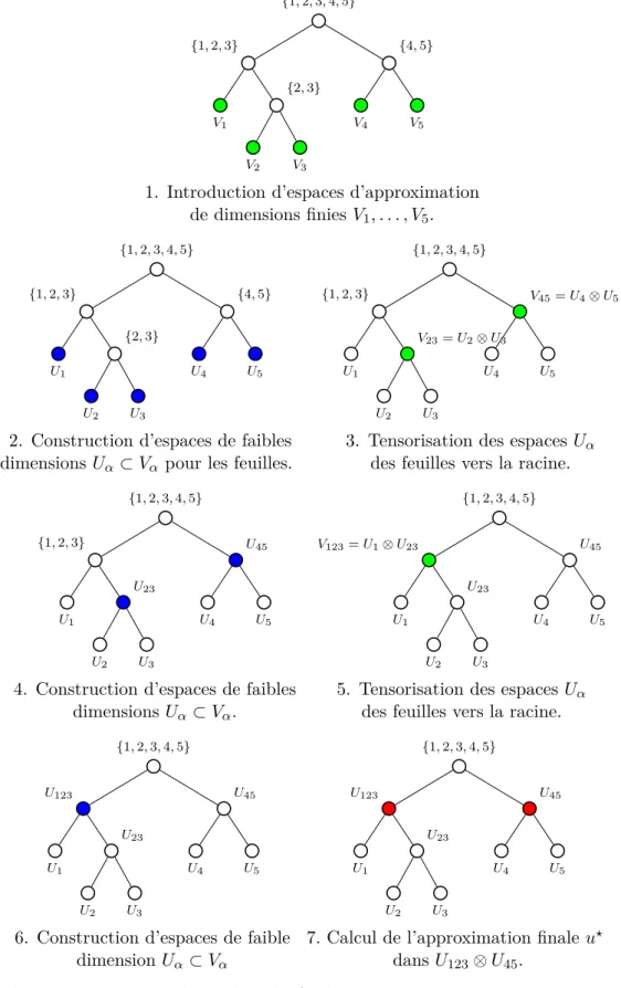
Le chapitre 5 fournit un algorithme adapté de [78] pour construire l’approximation dans un format de tenseur basé sur des arbres TT
r (H). En utilisant une approche allant des feuilles à la
racine, l’algorithme construit grâce à l’analyse en composantes principales (ACP) séquentiellement le long de l’arbre de dimension T , des sous-espaces de faible dimension de fonctions de groupes de variables associés à chaque noeud de l’arbre. Une illustration du principe de l’algorithme est donnée dans Figure 3. Nous analysons l’algorithme dans le cas où la projection vérifie une propriété de stabilité et dans le cas particulier de la projection des moindres carrés optimaux boostés. En utilisant cette stratégie, l’erreur d’approximation a plusieurs contributions venant de la discrétisa-tion (due à H), de la troncature (due à l’approximadiscrétisa-tion de faible rang) et de l’estimadiscrétisa-tion (due au nombre limité d’échantillons). Nous proposons un algorithme adaptatif partiellement heuristique
qui contrôle simultanément les erreurs de discrétisation, de troncature et d’estimation.
L’algorithme proposé au chapitre 5 fonctionne pour toute fonction u et tout arbre de parti-tion de dimension T . Cependant, les rangs et donc le nombre d’évaluaparti-tions n nécessaires pour atteindre une précision donnée peuvent dépendre fortement de l’arbre choisi T . Le choix de l’arbre qui minimise le nombre d’évaluations n pour une précision donnée est un problème d’optimisation combinatoire qui ne peut pas être résolu en pratique. Dans [48], les auteurs proposent un algo-rithme stochastique qui explore un nombre raisonnable d’arbres de dimension avec la même arité (nombre maximal d’enfants que des noeuds d’un arbre). L’idée clé est de favoriser l’exploration des arbres conduisant à des faibles rangs. Dans [10], les auteurs proposent une stratégie détermin-iste qui construit un arbre de dimension des feuilles à la racine par concaténation successive des nœuds, comme le suggère la Figure 4. Les regroupements sont décidés de manière à minimiser une certaine fonctionnelle des α-rangs estimés. L’arbre sélectionné peut alors être utilisé pour calculer l’approximation de u. Au nombre d’évaluations nécessaires pour calculer l’approximation s’ajoute le nombre d’évaluations de la fonction utilisée pour estimer les α-rangs. Ces deux coûts doivent être pris en compte pour évaluer l’efficacité d’une stratégie. Dans le chapitre 6, nous proposons trois stratégies adaptatives différentes pour réaliser l’optimisation de l’arbre. Une stratégie stochastique globale inspirée de [48] qui explore plusieurs arbres de dimension et sélectionne celui qui minimise une fonctionnelle des α-rangs estimés. Les deux autres stratégies incluent l’optimisation des arbres à l’intérieur de l’algorithme de construction de l’approximation présentée au chapitre 5. Au fur et à mesure que l’algorithme va des feuilles à la racine, le nombre d’arbres possibles (et donc le nombre de α-rangs à évaluer) diminue fortement. C’est pourquoi nous proposons (en plus de la stratégie stochastique) une stratégie déterministe (qui permettra d’explorer un plus grand nombre d’arbres).
{1, 2, 3, 4, 5} {1, 2, 3} V1 {2, 3} V2 V3 {4, 5} V4 V5
1. Introduction d’espaces d’approximation de dimensions finies V1, . . . , V5. {1, 2, 3, 4, 5} {1, 2, 3} U1 {2, 3} U2 U3 {4, 5} U4 U5
2. Construction d’espaces de faibles dimensions Uα⊂ Vα pour les feuilles.
{1, 2, 3, 4, 5} {1, 2, 3} U1 V23= U2⊗ U3 U2 U3 V45= U4⊗ U5 U4 U5
3. Tensorisation des espaces Uα
des feuilles vers la racine.
{1, 2, 3, 4, 5} {1, 2, 3} U1 U23 U2 U3 U45 U4 U5
4. Construction d’espaces de faibles dimensions Uα ⊂ Vα. {1, 2, 3, 4, 5} V123= U1⊗ U23 U1 U23 U2 U3 U45 U4 U5
5. Tensorisation des espaces Uα
des feuilles vers la racine.
{1, 2, 3, 4, 5} U123 U1 U23 U2 U3 U45 U4 U5
6. Construction d’espaces de faible dimension Uα⊂ Vα {1, 2, 3, 4, 5} U123 U1 U23 U2 U3 U45 U4 U5
7. Calcul de l’approximation finale u⋆
dans U123⊗ U45.
Figure 3 – Illustration de l’algorithme allant des feuilles à la racine du chapitre 5 pour la construction de l’approximation d’une fonction dans un format de tenseur basé sur des arbres.
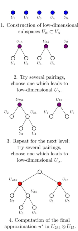
U1 U2 U3 U4 U5
1. Construction d’espaces de faibles dimensions Uα⊂ Vα U15 U1 U5 U34 U3 U4 U2
2. Test de plusieurs configurations de paires, et choix de celle qui donne
des espaces Uα de faibles dimensions. U234
U2 U34
U3 U4
U15
U1 U5
3. Recommencer pour le niveau suivant: test de plusieurs configurations de paires,
et choix de celle qui donne des espaces de faibles dimensions Uα.
U234 U1 U23 U2 U3 U15 U1 U5
4. Calcul de l’approximation finale u⋆
dans U234⊗ U15.
Figure 4 – Construction de l’arbre des feuilles vers la racine avec optimisation locale des regroupe-ments.
Context
Thanks to computational models, researchers and engineers are able to replace expensive physical experiments by numerical simulations. The response of a model depending on some parameters can be represented by a function u(x1, . . . , xd) of several variables. Despite the continuous
improve-ment of hardware resources, most of these simulations remain very costly to compute. Furthermore, solving uncertainty quantification (UQ) problems, which include in particular forward uncertainty propagation, model calibration, inverse problems or sensitivity analysis [87, 34], require a high num-ber of model’s evaluations. One remedy is then to replace the costly model by a surrogate model, cheaper to evaluate, which amounts in approximating the function that represents the model’s response.
The goal of approximation is to replace a function u by a simpler one (i.e. easier to evaluate) such that the distance (measuring the quality of the approximation) between the function u and its approximation, denoted u⋆, is as small as possible. In general, the approximation is searched in
a subspace of functions Vm described by a number of parameters m. A sequence of such subspaces
(Vm)m≥1 is called an approximation tool (or a model class), whose complexity is measured by its
number of parameters m. The error of best approximation of u by an element of Vm is defined by
the minimal distance between u and any element of Vm. The approximation tool should be adapted
to the class of functions we want to approximate, meaning that the error of best approximation should converge to zero quickly enough with m.
There exist different approaches to construct a function’s approximation either based on direct information on the function (e.g. point evaluations, linear measurements...) or equations satisfied by the function. In this thesis, we are interested in black-box (possibly noisy) functions (which corresponds to the first situation where the information on u is given by samples). Therefore, to construct the approximation of the function u, we rely on evaluations yi = u(xi) for a set of points
xi or yi= u(xi) + ei in the noisy case. However, in the context of costly model, this approximation
should be constructed using a reduced number of samples, ideally close to the number of parame-ters m. The samples xi may either be independent and identically distributed from a measure µ
or adaptively selected. This second situation is particularly relevant when no function’s evaluation has already been made and this will be the framework for this thesis.
Typical methods to construct a sample-based approximation are interpolation and least-squares methods [28]. Classical interpolation methods include polynomial and spline interpolation (where the samples are in general chosen relatively to Vm, to ensure good properties of the interpolation
operators), as well as kriging (which is quite efficient when the samples are given and may be improved with adaptive selection of the samples) [82]. For a given set of m points, x1, . . . , xm the
interpolation u⋆ of u in V
m is defined by
u(xi) = u⋆(xi), for all 1 ≤ i ≤ m.
Interpolation is well-studied in the one-dimensional case, see for example [57], but in the multivari-ate case (d > 1), finding good points for the interpolation is a challenging problem, in particular when Vm is a non-classical approximation space. In practice, for sparse polynomial or tensor
prod-uct spline interpolation, [18, 19, 16] propose strategies to constrprod-uct good sequences of interpolation points. However, for non-classical approximation spaces, even if some sets of points have shown their efficiency (see [65, 15]), there is no associated guarantee on the resulting distance between u and its interpolation.
Given n samples x1, . . . , xnindependent and identically distributed from a measure µ, standard
least-squares methods define the approximation of u as the minimizer of
min v∈Vm 1 n n X i=1 (v(xi) − yi)2.
An interesting aspect of least-squares methods is that they are able, under conditions on the num-ber of samples n, to guarantee a stable approximation and an error close to the best approximation error measured in L2
µ norm. However, to do so, they may require a sample size n much higher
than m (see [70, 22, 69, 93, 1]). Least-squares methods are a particular case of empirical risk minimization in supervised learning [30]. Other functionals can be used in this risk minimization, but they also require many evaluations in order to ensure the stability.
When the samples xi can be selected, the estimation error can be improved using weighted
least-squares [32, 73], by solving min v∈Vm 1 n n X i=1 wi(v(xei) − yi)2,
where the weights are adapted to Vm and the pointsxei are independent and identically distributed
same approximation error, compared to standard least-squares. In [24], the authors introduce an optimal sampling measure whose density with respect to the reference measure depends on the approximation space Vm. In [68], a similar optimal sampling approach is proposed whose major
difference is that the random samples are more structured than in [24]. They both show that the weighted least-squares projection built with samples from this measure is stable in expectation under a milder condition on n compared to classical least-squares. Nevertheless, to ensure the sta-bility of the weighted projection, these two optimal sampling measures still require a high number of samples n, compared to an interpolation method. The authors also propose optimal weighted least-squares methods in the case of adaptive approximation (when Vm is picked in a sequence of
nested approximation spaces), see [68] and [4]. In this thesis, we propose a new projection method onto a fixed approximation space Vm which ensures the stability of the least-squares projection in
expectation with a sample size close to m. We also propose a new method for the adaptive setting which significantly reduces the number of samples and still presents stability properties.
In many applications, functions may depend on a potentially high number of variables d ≫ 1. When the dimension d increases, using standard approximation tools adapted to smooth functions (e.g. splines for Sobolev functions) leads to a complexity of the approximation methods which grows exponentially with d. This is the so-called curse of dimensionality, expression introduced in [12]. As a consequence, the number of evaluations necessary to approximate the function u with naive approximation tools may explode. In this thesis, we assume that the functions present some low-dimensional structures, so that we can expect a good approximation using a limited number of evaluations of the function. Exploiting these structures of the function usually requires particular approximation tools [29], which may be application dependent. Some of the most usual ones are detailed hereafter.
A first approach consists in using the sparsity of u by choosing a particular set of functions {ϕj}j∈Λ among a set of tensorized bases functions, such that u(x) can be written as an expansion
P
j∈Λajϕj(x). Sparse approximation methods have been considered for solving uncertainty
quan-tification problems, see e.g. [23, 6, 5, 18, 19, 74, 75] for sparse polynomial approximation.
More structured model classes to deal with high-dimensional problems are additive models, introduced by [41], Pd
i=juj(xj) or more generally Pα∈Tuα(xα) where T ⊂ 2{1,...,d} is either fixed
(this corresponds to linear approximation) or a free parameter (this corresponds to non-linear ap-proximation). There are also multiplicative models Qd
j=1uj(xj) or more generally Qα∈Tuα(xα),
where T is also a subset of 2{1,...,d} and the same distinction between linear and non-linear
approx-imation is made, depending if T is fixed or not. These types of approxapprox-imation tools are standard in statistics and probabilistic modelling (graphical models, bayesian networks).
Furthermore, more complex model classes based on compositions of functions have been pro-posed. Among them ridge models can be written under the form v(W x) with W ∈ Rk×d, where
v belongs to a model class of functions of k variables with a low-dimensional parametrization. A typical example is the perceptron aσ(wTx+b), where σ is a given activation function, introduced in
[83]. These compositional models also include projection pursuit models of the formPk
j=1vj(wTjx),
where for j = 1, . . . , k, wj ∈ Rd, [41, 42], a particular case being neural networks with one hidden
layerPd
j=1ajσ(wjTx + bj). More general compositions of functions vL◦vL−1◦. . .◦v1 have been
con-sidered. They include the trendy deep neural networks, which are such that for each j = 1, . . . , L, the functions vj write vj(t) = σ(Ajt + bj), where σ is a chosen activation function, while bj ∈ Rk
and Aj ∈ Rk×d are parameters to estimate [45]. In spite of its general formalism and the many
successes that it has acquired in approximation, the use of deep neural networks generally requires a high number of evaluations to learn the parameters, which is not affordable in the context of costly evaluations. Furthermore, when considering general non-linear activation functions, it is difficult to guarantee a stable approximation whose error is close to the best approximation error, which is a central objective of this thesis.
In this work, we focus on the model class of rank-structured functions and in particular on the set of functions in tree-based tensor formats or tree tensor networks, which can be seen as a particular class of neural networks. More specifically, for α a subset of D = {1, . . . , d} and αc= D \ α its complementary subset in D, we focus on functions that can be written as
v(x) = rα X i=1 uαi(xα)uα c i (xαc), for all α ∈ T, (1)
where T is a dimension partition tree, which is a particular collection of subsets of D. Some exam-ples of dimension trees are given in Figure 1. The minimal integer rα such that v can be written
under the form (1) is called the α-rank of v, denoted rankα(v). The set of functions in tree-based
tensor format is defined by TT
r (H) = {v ∈ H : rankα(v) ≤ rα, α∈ T }, with r = (rα)α∈T a tuple of
integers, and H some approximation space of multivariate functions. It includes the Tucker format for a trivial tree, the tensor-train format for a linear binary tree [79] and the more general hierarchi-cal format for a general dimension partition tree [54]. Any function in TT
r (H) admits a multilinear
parametrization with parameters forming a tree network of low-order tensors, hence the name tree tensor networks, see Figure 2 for an illustration in the case where d = 5. Considering dimension trees for T gives nice topological and geometrical properties to the model class TT
r (H) [35, 37]. Tree
tensor networks are particularly relevant for high-dimensional approximation, because the complex-ity of the parametrization of a function in tree-based tensor format is linear in the dimension d and polynomial in the ranks [53]. It can also be used for one-dimensional approximation [2, 3].
{1, 2, 3, 4, 5} {1} {2} {3} {4} {5} Trivial tree {1, 2, 3, 4, 5} {1, 2, 3, 4} {1, 2, 3} {1, 2} {1} {2} {3} {4} {5}
Linear binary tree
{1, 2, 3, 4, 5} {1, 2, 3} {1} {2, 3} {2} {3} {4, 5} {4} {5}
General binary tree
Figure 1 – Examples of dimension partition trees with d = 5.
However the ranks and therefore the number of evaluations n necessary to compute an approxi-mation in tree-based tensor format with a given tolerance may strongly depend on the chosen tree T . The model class TT
r (H) can also be interpreted as a class of functions that are compositions of
multilinear functions, the structure of compositions being given by the tree. It has been identified with a particular class of deep neural networks (more precisely sum-product networks or arithmetic circuits) with a sparse connectivity and without parameter sharing [26]. The approximation error associated to this model class has two contributions : the truncation error (due to the finite ranks r) and the discretization error (due to the introduction of finite-dimensional spaces H).
{1, 2, 3, 4, 5} {1, 2, 3} {1} {2, 3} {2} {3} {4, 5} {4} {5}
Figure 2 – A tree-based tensor network admits a multilinear parametrization with parameters forming a tree network of low-order tensors.
Tree tensor networks are an approximation tool that achieve good performances for many classes of functions. In [84] or more recently in [7, 2, 3], the authors show that for functions u with Sobolev
regularity, they achieve (whatever the tree is) an approximation rate which is optimal or close to optimal [61]. They also prove that for functions u with mixed Sobolev regularity, the approxi-mation in tree-based tensor format achieves almost the ideal performance obtained by hyperbolic cross approximation. For a literature review on low-rank approximation methods, see [47]. Also, we refer the reader to monograph [53] and surveys [8, 36, 59, 60, 77, 76].
In the literature, some algorithms constructing approximations in tree-based tensor formats us-ing points evaluations of functions have already been proposed. On the one hand, there are learnus-ing approaches that use random and unstructured evaluations of the functions [48, 55]. Robustness and effectiveness of such algorithms are observed on numerical experiments. However these algo-rithms are mainly based on heuristics and lack of theoritical analysis. On the other hand, there are algorithms that use adaptive and structured evaluations of tensors, see [64] (for the Tucker format), or [80] and [78] for tree-based tensor formats. Among adaptive approaches, the method from [78] is of particular interest, the author proposes a variant of higher-order singular value decomposition (HOSVD) (previous adaptations of HOSVD can be found in [46] and [80]). The principle is to construct a hierarchy of optimal subspaces that results in a final tensor product of subspaces in which the function u is projected, to define the final approximation u⋆. Under strong assumptions
on the estimation error made in the determination of subspaces, the author in [78] shows that with a number of evaluations scaling in the storage complexity of the tree-based tensor format, the approximation satisfies the desired error up to constants depending on some projection operators, which are not quantified.
All these conclusions show that theoretical results on the convergence of existing algorithms are limited. In this thesis we propose an algorithm that constructs an approximation u in tree-based tensor format, using adaptive and structured sampling with some theoretical guarantees, and we propose heuristic strategies for obtaining an approximation with a desired precision and near-optimal complexity.
Contributions
More precisely the contributions of this thesis can be summarized through the following objectives:
1. Propose a projection method in a linear space, based on sampling techniques, which is sta-ble and whose construction requires a number of evaluations close to the dimension of the approximation space.
2. Propose a strategy for computing linear projections onto a nested sequence of approximation spaces, using a reduced number of samples.
3. Propose a method to construct the approximation of a function in tree-based tensor format, with theoretical stability guarantees and propose heuristics to control the error.
4. Propose a strategy to choose the tree structure T in order to reduce ranks of the approximation at given precision and therefore its complexity and the required number of samples.
This thesis is divided into six chapters. Chapters 1 and 4 provide a state-of-the-art on projection methods onto linear approximation spaces and tree-based tensor formats respectively. Chapters 2, 3, 5 and 6 correspond to the main contributions of this thesis addressing the four objectives listed above. In the appendix implementation aspects for sampling multivariate probability distributions in tree-based tensor formats are given.
In Chapter 2, we propose a new projection method, called boosted optimal weighted least-squares method, that ensures stability of the least-least-squares projection with a sample size close to the interpolation regime n = m. It consists in sampling according to a measure associated with the optimization of a stability criterion over a collection of independent n-samples, and resampling ac-cording to this measure until a stability condition is satisfied. A greedy method is then proposed to remove points from the obtained sample. Quasi-optimality properties in expectation are obtained for the weighted least-squares projection, with or without the greedy procedure. If the observations are polluted by a noise, quasi-optimality property is lost, because of an additional error term due to the noise. This latter error term can however be reduced by increasing n.
In order to control the approximation error, we should be able to choose the approximation space adaptively (with a dimension high enough to reach a certain accuracy). For polynomial approximation and applications in UQ, several strategies to construct adaptively a sequence of approximation spaces (Vml)l≥1 have been proposed in [43, 67, 18, 19]. To limit the total number of
evaluations of the function, it is necessary to reuse the samples used to build the projection onto the space Vml in order to construct the one onto the space Vml+1. However, the optimal weighted
boosted least-squares projection from Chapter 2 depends on the approximation space, such that reusing the samples used to construct a projection to construct another is not straightforward. In [68], the author proposes an adaptive optimal weighted least-squares method that recycles all samples from one step to another. In Chapter 3, we propose an adaptive boosted optimal weighted least-squares method inspired from [68], using again resampling, conditioning and greedy proce-dures. This strategy works for a general sequence of nested approximation spaces and we apply it for adaptive sparse polynomial approximation.
Chapter 5 provides an algorithm adapted from [78] to construct the approximation in a tree-based tensor format TT
a series of principal component analyses (PCA) along the tree structure T , low-dimensional sub-spaces of functions of groups of variables associated with each node of the tree. This algorithm is illustrated by the Figure 3. We analyse the algorithm in the case where the projection verifies a stability property and in the particular case where the projection is the boosted least-squares pro-jection. Using this strategy the approximation error has several contributions due to discretization (due to H), truncation (due to low-rank approximation) and estimation (due to the limited number of samples). We propose a partially heuristic adaptive algorithm that controls simultaneously the discretization, truncation and estimation errors.
The proposed algorithm from Chapter 5 works for any function u and any dimension partition tree T . However the ranks and therefore the number of evaluations n necessary to reach a given precision may strongly depend on the chosen tree T . Choosing the tree which minimizes the number of evaluations n for a given accuracy is a combinatorial optimization problem and it is not feasible in practice. In [48], the authors propose a stochastic algorithm that explores a reasonable number of dimension trees with the same arity (maximal number of children of any node of a tree). The key idea is to favour the exploration of trees yielding low ranks. In [10], the authors propose a deterministic strategy that constructs a dimension tree in a leaves-to-root approach by successive concatenations of nodes. The groupings are decided in order to minimize a certain functional based on estimated α-ranks. The selected tree can be used to compute the approximation of u. The number of function’s evaluations used to estimate the α-ranks adds up to the number of evaluations necessary to compute the approximation. This total number of samples should be used to evaluate the efficiency of a strategy. In Chapter 6, we propose three different adaptive strategies to perform tree optimization. A global stochastic strategy inspired from [48] which explores several dimension trees and select the one minimizing a complexity functional depending on α-ranks estimations. The two other strategies include tree optimization inside the algorithm for the construction of the approximation presented in Chapter 5, as suggested in Figure 4. As the algorithm goes from the leaves to the root, the number of possible trees (and thus the number of α-ranks to be evaluated) decreases sharply. This is why we propose (in addition to the stochastic strategy) a deterministic strategy (which will explore a larger number of trees).
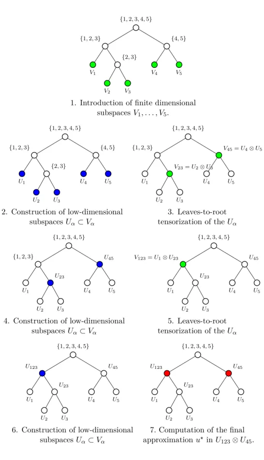
{1, 2, 3} V1 {2, 3} V2 V3 {4, 5} V4 V5
1. Introduction of finite dimensional subspaces V1, . . . , V5. {1, 2, 3, 4, 5} {1, 2, 3} U1 {2, 3} U2 U3 {4, 5} U4 U5 2. Construction of low-dimensional subspaces Uα⊂ Vα {1, 2, 3, 4, 5} {1, 2, 3} U1 V23= U2⊗ U3 U2 U3 V45= U4⊗ U5 U4 U5 3. Leaves-to-root tensorization of the Uα {1, 2, 3, 4, 5} {1, 2, 3} U1 U23 U2 U3 U45 U4 U5 4. Construction of low-dimensional subspaces Uα⊂ Vα {1, 2, 3, 4, 5} V123= U1⊗ U23 U1 U23 U2 U3 U45 U4 U5 5. Leaves-to-root tensorization of the Uα {1, 2, 3, 4, 5} U123 U1 U23 U2 U3 U45 U4 U5 6. Construction of low-dimensional subspaces Uα ⊂ Vα {1, 2, 3, 4, 5} U123 U1 U23 U2 U3 U45 U4 U5
7. Computation of the final approximation u⋆ in U
123⊗ U45.
subspaces Uα ⊂ Vα U15 U1 U5 U34 U3 U4 U2
2. Try several pairings, choose one which leads to
low-dimensional Uα. U234 U2 U34 U3 U4 U15 U1 U5
3. Repeat for the next level: try several pairings, choose one which leads to
low-dimensional Uα. U234 U2 U34 U3 U4 U15 U1 U5
4. Computation of the final approximation u⋆ in U
234⊗ U15.
P
ROJECTION METHODS
Contents
1.1 Introduction . . . . 29 1.2 Interpolation . . . . 29 1.2.1 Interpolation in the one-dimensional case . . . 31 1.2.2 Interpolation with any arbitrary approximation space . . . 33 1.2.3 Interpolation with tensor product bases . . . 34 1.3 Least-squares method . . . . 35 1.3.1 Weighted least-squares projection . . . 36 1.3.2 Random sampling . . . 38 1.3.3 Optimal sampling measure . . . 40
1.1
Introduction
In this chapter we present two classical families of methods to construct the approximation of a function onto a linear space Vm, using evaluations of the function at suitably chosen points:
inter-polation and least-squares regression [28].
The outline of this chapter is as follows. In Section 1.2, we present the approximation of mul-tivariate functions by interpolation. In Section 1.3, we present weighted least-squares projections. Then, we recall the optimal sampling measure from [24], and outline its limitations.
1.2
Interpolation
In this section, we begin by recalling the definition of interpolation of a real-valued function u defined on a subset X ⊂ Rd onto an approximation space V
We consider a m-dimensional linear space Vm whose basis is denoted {ϕj}mj=1, where the ϕj can
be polynomials, splines or wavelets for instance. We denote by
ϕ= (ϕ1, . . . , ϕm) : X → Rm
the m-dimensional vector-valued function such that ϕ(x) = (ϕ1(x), . . . , ϕm(x))T.
Let Γm = {xi}mi=1 be a set of m points in X . The interpolation of u is defined as the
approxi-mation u⋆ ∈ V
m such that
u⋆(xi) = u(xi) for all xi ∈ Γm.
u⋆ can be written under the form
u⋆(x) =
m
X
j=1
ajϕj(x),
where the coefficients (aj)m
j=1 are solution of the following linear system,
ϕ1(x1) ϕ2(x1) . . . ϕm(x1) ϕ1(x2) ϕ2(x2) . . . ϕm(x2) . . . ϕ1(xm) ϕ2(xm) . . . ϕm(xm) | {z } Vϕ(x1,...,xm) a1 a2 .. . am = u(x1) u(x2) .. . u(xm) .
Here, the matrix Vϕ(x1, . . . , xm) is called the Vandermonde like-matrix. We say that Γm is
uni-solvent for the space Vm = span{ϕj}mj=1 if Vϕ(x1, . . . , xm) is invertible, which implies that u⋆ is uniquely defined for any u. A set of points that maximizes the determinant of the Vandermonde-like matrix Vϕ(x1, . . . , xm) is called a set of Fekete points [40]. If Γm is unisolvent, the interpolation
operator Im : X → Vm is defined by Imu = u⋆ and the associated Lebesgue constant Lm (in L∞
norm) is defined by Lm= kImk = sup v6=0 kImvkL∞ kvkL∞ . It holds ku − u⋆kL∞ ≤ (1 + Lm) inf v∈Vmku − vkL ∞.
The Lebesgue constant Lm can be expressed in terms of interpolation functions, but in general an
expression of Lm can not be explicitly found. In dimension one, interpolation is well understood
for various types of approximations (e.g. with polynomials, splines). In particular for polynomial spaces Vm there exists good sets of points Γm, such that the Lebesgue constant Lm is controlled.
Some of them are detailed in Section 1.2.1. However in higher dimension, finding good points for polynomial approximation is a challenging problem. In Section 1.2.2, we consider the
multivari-ate setting and present several sets of interpolation points that have demonstrmultivari-ated their efficiency in practice. In Section 1.2.3, we consider the case where the approximation space is constructed from tensor product bases and present the construction of interpolation operator for approximation spaces associated to downward closed index sets. The purpose of these three sections is not to give an exhaustive list of already studied interpolation points but an insight on the most classical inter-polation points and in particular the ones to which we will compare the boosted optimal weighted least-squares method, contribution of this thesis.
1.2.1 Interpolation in the one-dimensional case
In this subsection, we recall some well-known results for one-dimensional polynomial interpolation i.e. with Vm a space of degree m − 1 polynomials. A lower bound for the Lebesgue constant is
given by the Erdos theorem [33], which shows that in the best case, Lm grows as the logarithm of
the dimension m. More precisely for any set of points, there exists a constant C > 0 such that,
Lm ≥ 2
πlog(m + 1) − C.
Uniformly distributed points.
For uniformly distributed points over [−1, 1], it holds
Lm ∼ 2 m+1
em log(m) as m → ∞,
that shows that uniformly distributed points is clearly not a good option for interpolation.
Chebyshev points.
Another classical set of points is the Chebyshev set of points, which is defined as the solution of
min x1,...,xmx∈[−1,1]max m Y j=1 |x − xj|.
For a given m, these points are near optimal asymptotically according to the Erdos theorem, since
Lm ∼ 2
πlog(m) as m → ∞.
However, Γm 6⊂ Γm+1 (i.e the set of the m Chebyshev points is not included in the set of m + 1
Gauss-quadrature type points.
When the approximation space Vm is the span of the univariate Legendre polynomials {ϕj}mj=1,
the Gauss-Legendre points are well-suited for interpolation. For 1 ≤ i ≤ m, the ith point of the
Gauss-Legendre set of m points is given by the ith root of ϕ
m, the Legendre polynomial of degree
m− 1. The Lebesgue constant for the point set consisting of the Gauss-Legendre points is
Lm ≤ C√m, see [88].
Similarly, when the approximation space is the span of the Hermite polynomials, the Gauss-Hermite points can be defined as the roots of the Hermite polynomials.
Clenshaw-Curtis points.
Clenshaw-Curtis points are the extrema of Chebyshev polynomials. For m ≥ 1, the sequence of m Clenshaw-Curtis points is given by Γm = {cos(m−1jπ ) : j = 0, . . . , m − 1} and the Lebesgue constant
verifies
Lm≤ 2
π log(m − 1) + 1.
The interest is that Γ2m ⊂ Γ2m+1, which is useful for adaptive approximation. But this requires to
double the dimension of the approximation space at each iteration.
Leja points.
Another sequence of points which is suitable for adaptive approximation is the Leja sequence, which is defined recursively for j ≥ 2 by
xj ∈ arg max x∈[−1,1] j Y l=1 |x − xl|,
with x1 taken equal to 0 or 1 in general. The definition is such that this sequence is not unique.
An equivalent definition for the Leja sequence of points is given by
xj ∈ arg max
x∈[−1,1]|detVϕ(x
1, . . . , xj−1, x)| for j ≥ 2.
Therefore Leja sequences can be seen as a greedy D-optimal experimental design [38]. It does not exist any explicit expression for the Lebesgue constant associated to this set of points, but it has been proven that it grows subexponentially [39].
R-Leja points are real part of the Leja points defined on the complex unit disc. In other terms, they are defined as the projection on the real line of complex Leja points. In dimension one, it has
been proven (see [21]) that
Lm≤ C(m + 1)2.
1.2.2 Interpolation with any arbitrary approximation space
Leja points.
The definition of the Leja points can be extended to the cases where d > 1, for any compact set E of Rd [66], for k ≥ 2, by
xk∈ arg max
x∈E| det Vϕ(x
1, . . . , xk−1, x)|.
When d is high, this sequence of points may be costly to compute, therefore it can be replaced by a so-called sequence of discrete Leja points which relies on a LU factorization with row-pivoting of the Vandermonde-like matrix [15]. To deal with the case of unbounded domains, weighted versions of discrete Leja points have been proposed [16].
Fekete points.
A set of points that maximizes the determinant of the Vandermonde-like matrix Vϕ(x1, . . . , xm) is called a set of Fekete points [40]. These points are not limited to polynomial approximation but can be used in a very general setting. In general they are very expensive to compute because it requires a multivariate optimization. Therefore methods to compute approximate Fekete points based on QR factorizations with column pivoting of the Vandermonde-like matrix have been proposed in [86], [14] and [15]. To deal with the case of unbounded domains, weighted Fekete points have also been introduced [51]. There exist connections between Leja and Fekete points [66].
Magic points.
In [65], the authors propose a sequence of interpolation points called magic points which provides in practice good results in terms of the behaviour of the Lebesgue constant. An interest of this method is that it is not limited to polynomial approximation. Furthermore, these points can be relatively simply determined through a greedy algorithm. The procedure is as follows: we start from a candidate set of points Γ and determine a first point x1 and an index i
1 such that
|ϕi1(x
1)| = max
Then for k ≥ 1, we define e ϕki(x) = ϕi(x) − k X l=1 k X p=1 ϕil(x)a k l,pϕi(xp),
with the matrix A = (ak
l,p)1≤l,p≤k being the inverse of the matrix
ϕi1(x 1) ϕ i2(x 1) . . . ϕ ik(x 1) ϕi1(x2) ϕi2(x2) . . . ϕik(x 2) . . . ϕi1(x k) ϕ i2(x k) . . . ϕ ik(x k) ,
such that ϕekil(x) = 0 for all 1 ≤ l ≤ k and x ∈ X andϕeki(xp) = 0 for all 1 ≤ p ≤ k and 1 ≤ i ≤ m.
Then we determine the point xk+1∈ Γ and an index i
k+1 such that
|ϕekik+1(xk+1)| = max
x∈Γ 1≤i≤mmax |ϕe
k i(x)|.
The Lebesgue constant associated with the magic points behaves relatively well in practice [92].
1.2.3 Interpolation with tensor product bases
In this subsection, we consider the case where X has a product structure X = X1× . . . × Xd, then
multivariate interpolation on tensor product bases can be constructed from univariate interpolation.
For each k ∈ {1, . . . d}, we consider {ψk
ik}ik≥1 a set of univariate functions defined on Xk. We
define for all i = (i1, . . . , id) ∈ Nd,
ϕi(x) = d
Y
k=1
ψkik(xk). (1.1)
Let us introduce a set of multi-indices Λm ⊂ Nd such that #Λm = m. The set Λm ⊂ Nd is
said to be downward closed if for all α ∈ Λm and any β such that β ≤ α (i.e. for all 1 ≤ k ≤ d,
βk ≤ αk), then β ∈ Λm. We introduce Vm the associated approximation space
Vm = span{ϕi: i = (i1, . . . , id) ∈ Λm}.
Furthermore, for each k ∈ {1, . . . d}, we consider {xik
k} mk
ik=1 a sequence of points in Xk unisolvent
for the basis {ψk ik}
mk
ik=1, therefore defining a unique interpolation operator denoted I
k