HAL Id: inria-00092408
https://hal.inria.fr/inria-00092408
Submitted on 9 Sep 2006HAL is a multi-disciplinary open access
archive for the deposit and dissemination of sci-entific research documents, whether they are pub-lished or not. The documents may come from
L’archive ouverte pluridisciplinaire HAL, est destinée au dépôt et à la diffusion de documents scientifiques de niveau recherche, publiés ou non, émanant des établissements d’enseignement et de
operator by a stochastic method
Antoine Lejay, Sylvain Maire
To cite this version:
Antoine Lejay, Sylvain Maire. Computing the principal eigenvalue of the Laplace operator by a stochastic method. Mathematics and Computers in Simulation, Elsevier, 2007, 73 (3), pp.351-363. �10.1016/j.matcom.2006.06.011�. �inria-00092408�
operator by a stochastic method
Antoine Lejay1,† —Projet OMEGA, INRIA & Institut ´Elie Cartan, Nancy
Sylvain Maire2 — ISITV, Univ. de Toulon et du Var, Toulon
Abstract: We describe a Monte Carlo method for the numerical computation of the principal eigenvalue of the Laplace operator in a bounded domain with Dirichlet conditions. It is based on the estimation of the speed of absorption of the Brownian mo-tion by the boundary of the domain. Various tools of statistical estimation and different simulation schemes are developed to op-timize the method. Numerical examples are studied to check the accuracy and the robustness of our approach.
Keywords: First eigenvalue of the Dirichlet problem, Euler scheme for Brownian motion, random walk on spheres, random walk on rectangles
AMS Classification: 65C05, 60F15
Published in Mathematics and Computers in Simulations. In print
Archives, links & reviews:
◦ doi: 10.1016/j.matcom.2006.06.011 1Current address: Projet OMEGA (INRIA/IECN)
IECN
Campus scientifique BP 239
54506 Vandoeuvre-l`es-Nancy CEDEX, France E-mail: [email protected]
2Current address: ISITV, Universit´e de Toulon et du Var
Avenue G. Pompidou BP 56
83262 La Valette du Var CEDEX, France E-mail: maire@u vni -tln.fr
†Partially supported by GdR MOMAS (financed by the institutes
1
Introduction
The aim of this paper is to introduce and study a Monte Carlo method for the numerical computation of the principal eigenvalue of the Laplace oper-ator 1
24 in a bounded domain D ⊂ <d with a sufficiently piecewise smooth
boundary ∂D and with Dirichlet boundary conditions. This leading eigen-value determines the speed of convergence to the steady state for the solution of the heat equation. To compute it by a deterministic method, one has to discretize the Laplace operator using for example finite differences or finite elements and then evaluate the largest eigenvalue of the discretization ma-trix using for example the inverse power method. This computation becomes really expensive when the spatial dimension d increases. Moreover the dis-cretization should be refined enough so that the principal eigenvalue of the discretization matrix is close enough to the principal eigenvalue of the Laplace operator. Hence it is worth considering Monte Carlo methods [15] because they are usually efficient for this kind of difficult problems since they do not necessarily require to discretize the domain D and they depend only linearly on the spatial dimension.
We have introduced in [17] a stochastic method to compute the principal eigenvalue of neutron transport operators based on the numerical computa-tion of the type of the neutron transport operator. The idea was to combine the formal eigenfunction expansion of the solution of the relative Cauchy problem and its Monte Carlo evaluation via the Feynman-Kac formula. We intend to use the same methodology here in the case of the Laplace operator. The stochastic representation of the principal eigenvalue of the operator 1
24
is usually achieved by combining the solution u(t, x) of the Cauchy problem
∂u ∂t = 1 24u, u(0, x) ≡ 1, x ∈ D ⊂ Rd
obtained by the Feynman-Kac formula and the formal eigenfunction expan-sion u(t, x) = ∞ X j=1 cjexp(λjt)Ψj(x)
of this solution in L2(D) where λj are the eigenvalues of 1
24 arranged in
decreasing order and Ψj their relative eigenfunctions. Indeed as the solution of this equation is given by
u(t, x) = P (τDx > t) ,
where τx
D is the exit time from D of the Brownian motion starting at x, the principal eigenvalue λ1 is directly linked to the speed of absorption of the
Brownian motion by the boundary ∂D and we have for all x ∈ D λ1 = limt→+∞ 1 t log P (τ x D > t) .
This result is also true for a general elliptic operator A with Dirichlet bound-ary conditions in a bounded domain D, where τx
D is the exit time from D of the stochastic process Xx
t generated by A [7, 8, 13, 19]. We had to compute numerically the same quantity in [17] when studying homogeneous neutron transport operator. In this case, an exact simulation of transport processes involved in Feynman-Kac representations was possible. In the case of the Brownian motion, one has to use approximations based on various discretiza-tion schemes.
In Section 2, we describe quickly grid-free schemes, some of them common and some of them new, that can be used here. Then, we present in Section 3 different estimators for λ1 based on an accurate study of the eigenfunctions
expansion of the solution u(t, x). Some of these estimators were developed in [17] but we also introduced new ones based on correlation coefficients. In order to compare the different simulations schemes and the different estima-tors, we study in detail in Section 4 a bidimensional problem. We finally study in Section 5 more difficult problems in dimension 3 and 5 combining all the tools developed previously in order to show that our method is also relevant in these cases.
2
exit time simulation procedures
The aim of this section is to describe and compare some simulation schemes for the exit time of the Brownian motion in a bounded domain D with Dirich-let boundary conditions.
2.1
Euler schemes
The Euler scheme (see for example [14]) with discretization parameter ∆t writes
X0 = x, Xn+1 = Xn+
√
∆tYn
where the Yn are independent standard Gaussian random variables. To com-pute P (τx
D > t) one needs to compute simulations of τDx. With the crude
version, the simulation stops once Xn+1∈ Dc and τDx is approximated either by n∆t, (n +1
2)∆t or a slightly refined approximation based on the distances
dn = d(Xn, ∂D) and dn+1= d(Xn+1, ∂D). In any case, these approximations are of weak order √∆t and they overestimate this exit time. Indeed, the
main simulation error does not come from the error at the last step but from the possibility for the Brownian motion to leave the domain between step
n and n + 1 and be back into it at time (n + 1)∆t. It is possible to take
into account this possibility to obtain a scheme of weak order ∆t using the half-space approximation [9, 10]. An additional random test based on dnand
dn+1 is required. Taking a uniform random variable Un, the motion stops if exp à −2dndn+1 ∆t ! > Un.
It is still possible to introduce another refinement at the last step [3] which improves the accuracy but does not change the order of the scheme. In [11], another method is proposed that leads to the same order of convergence as in the half-space method. We only consider in the examples the naive version and the one using the half-space approximation, which we denote from now by the Improved Euler scheme.
2.2
Walk on spheres (WOS)
The simulation method based on the Euler schemes covers a wide range of elliptic and parabolic partial differential equations and can take into account the dependence of the drift and of the diffusion coefficients on the spatial variables. One only has to simulate a stochastic differential equation by means of this scheme instead of the Brownian motion. However, in the case of the heat equation some faster schemes are available. The walk on sphere schemes (WOS) [20] relies on the isotropy of the Brownian motion. This walk goes from x to the boundary ∂D from a sphere to another until the motion reaches an ε-absorption layer. The spheres are built so that the jumps are as large as possible. The radius of the next sphere from a starting point
xn is d(xn, ∂D) and the next point is chosen uniformly on this sphere. The average number of steps to exit from the domain is proportional to | log(ε)| [20]. As we want here to simulate τx
D, we need in addition to simulate the law
Y (r) of the exit time from a sphere of radius r starting at its center. Some
scaling arguments on the partial differential equation or on the Brownian motion show that r2Y (1) and Y (r) have the same law. Some analytical
expressions for the distribution function H(t) = P(Y (1) < t) are available. In dimension 2, we have for example [1]
H(t) = ∞ X k=1 2J0(0) jkJ1(jk) exp à −j2 kt 2 !
where J0 and J1 are Bessel functions and the jk are the positive zeros of J0.
series which can be difficult and costly. As we only need here to simulate Y (1) during all the walk, we tabulate the distribution function once and for all and use it for simulations. Note that we can either use its analytical expression to do it or Monte Carlo simulations based on the corrected Euler scheme with a small parameter and a huge number of simulations. The second method is especially efficient in higher dimensions.
Some refined versions (for example, the walk on spheres with shifted cen-tres [12]) allow faster absorption by the boundary, but also leads to simulate complex random variables.
2.3
Walk on rectangles (WOR)
In many practical situations (temperature evolution in a room, ...), the boundary is or can be approximated by a polygon. In this case, exact and fast simulations are possible.
The idea of the random walk on rectangles (WOR) is a generalization of the random walk on squares [4], that can be deduce from the algorithm given in [18] to simulate Stochastic Differential Equations (SDE). The idea is to simulate the exit time and position from a rectangle (or a parallelepiped in dimension greater than 2) by a Brownian motion. Unlike with a sphere, the random variables giving the exit time and position from a rectangle are not independent. Yet, as shown in [5], this could be achieved rather efficiently by proper conditioning and reducing the problem to simulate random variables related to the one-dimensional Brownian motion. The advantage of this method is that, unlike with the random walks of spheres and squares, the rectangles may be chosen prior to any simulation, since the Brownian motion can start from any point in it. In addition, it can be used even if a constant drift term is present, or to deal with Neumann boundary condition. Although it takes more time to simulate the exit time and position from a rectangle, the number of simulations is reduced. Of course, one has to use, when possible, rectangles for which at least one side corresponds to a boundary of D.
Let (B1, . . . , Bd) be a d-dimensional Brownian motion with the starting point (B1
0, . . . , B0d) = (x1, . . . , xd). We denote by Px the distribution of the
one-dimensional Brownian motion starting at x. We are interested in simu-lating its first exit time and position from the parallelepiped [−L1, L1]×· · ·×
[−Ld, Ld]. For that, we set τi = inf{t > 0 ; Bti 6∈ [−Li, Li]} for i = 1, . . . , d and we perform roughly the following operations:
(1) We draw a realization (θ1, y1) for (τ1, B1
τ1) under Px1. We set τ = θ1,
S1 = 1 and J = 1.
(2.1) We use a Bernoulli random variable to decide whether {τi < τ } or {τi ≥ τ } under P
xi.
(2.2) If we have decided that {τi < τ }, then we draw a realization (θi, yi) of (τi, Bi
τi) under Pxi given {τi < τ }. We set J = i, Si = 1
and τ = τi.
(2.3) Otherwise, we set Si = 0, ϕi = τ . (3) We set zJ = yJ.
(4) For i from 1 to d, do
(4.1) If Si = 1 and i 6= J then we simulate a realization zi of Bτi under Pxi given {τi = θi, Bτii = yi}.
(4.2) Otherwise, if Si = 0, then we simulate a realization zi of Biτ under Pxi given {τi ≥ ϕi}.
(5) The algorithm stops and returns the time τ and the position (z1, . . . , zd) on the boundary of the parallelepiped.
The involved distributions and the exact algorithm are detailed in [5].
2.4
Walk on rectangles with importance sampling
(WOR-IS)
This method, developed in [6], is a variation on the previous method. In-stead of simulating the exact couple exit time τ and exit position Bτ of a rectangle R for a Brownian motion B, we draw this exit time and posi-tion (θ, Z) using an arbitrary distribuposi-tion (of course, chosen to be simple), and we compute a weight w such that E(f (τ, Bτ)) = E(wf (θ, Z)) for any bounded, measurable function f defined on R+ × ∂R. Of course, for any
function g defined on R+× ∂D, the functional E(g(τDx, Bτx
D)) is then
evalu-ated by E(w1· · · wn∗g(θn∗, Zn∗)), where the (θi, Zi)’s are the successive exit
times and positions for a sequence of rectangles, the wi’s are their associated weights, and n∗ is the first integer for which Z
n∗ belongs to ∂D, or is close
enough to ∂D.
The advantage of this method over the WOR/WOS is that we are free to choose the distribution of (θ, Z), and then we can easily “constraint” the diffusion to go in some direction or condition it not to reach a part of the boundary of the domain. Thus, this method can be used to simulate Brow-nian motion or SDE in domains with complex geometries and to reduce the variance of the estimators that are computed. Moreover, this method is much
more faster than the WOR if we choose for (θ, Z) random variables that are easy to simulate. In addition, the weights are rather easily computed since they rely on the density of the first exit time and the position of a killed Brownian motion in the one-dimensional case.
However, this method suffers from a severe drawback in our case. The empirical distribution function FN(t) of F (t) = P(τDx < t) is constructed as follows. If (θ(i), w(i))
i=1,...,N are the simulated exit time from D with their associated weights w(i), then
FN(t) = 1 N N X i=1 w(i)χ [0,t)(θ(i)).
If FbN(t) is the empirical distribution function constructed with N inde-pendent random variables with the same law as τx
D, then Var(FbN(t)) = N−1F (t)(1 − F (t)). In our case, Var(FN(t)) = 1 N Var(w (1)χ [0,t)(θ(1))).
The problem is then to find a “strategy” for which Var(FN(t)) is smaller than Var(FbN(t)), at least when t is large enough. Unfortunately, we have not been able to find a good way to do so. For the sake of simplicity, we have adopted the following strategy. For each rectangle, each of its side is reached with a probability 1/4, the exit position is drawn using a uniform random variable on the side and the exit time is simulated using an exponential random variable of parameter 0.35 times the square of the length of the side that is not reached.
3
Estimators of the principal eigenvalue
3.1
Direct approximation
Using the formal eigenfunction expansion of u(x, t), we can write that almost everywhere 1 t log(P (τ x D > t)) = 1 t log(C1e λ1t+ C 2eλ2t+ · · · + Ckeλkt+ o(eλkt)), where C1 = c1Ψ1(x). The Krein-Rutman theorem [19] ensures that λ1 is
simple and C1 > 0. Then
1 t log P (τ x D > t) ' λ1+ log(C1) t + C2 C1 e(λ2−λ1)t t
keeping only the two dominant terms. The previous approximation shows that lim t→∞ 1 t log P (τ x D > t) = λ1
almost everywhere and it has been proved in [13] that it holds everywhere. Hence the Monte Carlo computation of t−1log P(τx
D > t) for large times
of-fers a first possibility to give a numerical approximation of λ1. Moreover we
can choose the starting point wherever we want. The most natural choice is to take this starting point in the center of the domain in order to make the trajectories last as long as possible. Even if we do so, we will see in some numerical examples that this direct method gives in fact a poor approxima-tion because the variance increases quickly with time. Indeed this involves the computation of the probability of rare events which become rarer and rarer as time increases. We now give some better estimators to overcome this difficulty.
3.2
Interpolation method
The previous expansion is constituted of a main term λ1 + t−1log(C1) and
of a term C2
C1
e(λ2−λ1)t
t which decays at an exponential rate the more quickly the first two eigenvalues are distant from each other. The difference λ2− λ1
is intrinsic to the domain. Nevertheless the choice of a starting point near the center of the domain makes the ratio C2/C1 smaller. This can be seen
for instance on the eigenfunctions expansion on square domains. Moreover, it is well known that the errors due to the discretization scheme are smaller for points away from the boundary. If we assume that t is large enough so that this term is negligible with respect to the others, we can compute easily λ1 using the Monte Carlo approximations p1 and p2 of respectively
p1 = P(τDx,S > t1) and p2 = P(τDx,S > t2) with a discretization scheme S. We
obtain the estimators
λIn(t
1, t2) =
log(p2) − log(p1)
t2− t1
of λ1 which are also used in neutron transport criticality computations [2].
Note that p1 and p2 are obviously correlated and may also be biased esti-mators of P (τx
D > t1) and P (τDx > t2) because of the discretization errors.
Letting s1 =
q
p1(1 − p1), we obtain the 95 percent confidence interval
p1− 1.96√s1
N ≤ p1 ≤ p1+ 1.96
s1
√ N
that is assuming that s1 p1 √ N is small enough, log(p1) − 1.96 s1 p1√N ≤ log(p1) ≤ log(p1) + 1.96 s1 p1√N.
We finally have the 90 percent confidence interval for λIn(t
1, t2) writing log(p2 p1) t2− t1 − 1.96N− 1 2 t2 − t1 Ã s1 p1 + s2 p2 ! ≤ λIn(t1, t2) ≤ log(p2 p1) t2 − t1 +1.96N −1 2 t2− t1 Ã s1 p1 + s2 p2 ! . (1)
3.3
Least squares approximations
In order to make a global use of the information given by the computation of the solution at the different times, we can give a least squares approximation of λ1 and log(K0) by fitting these parameters to the approximation model
still assuming that the term C2
C1
e(λ2−λ1)t
t is negligible. We denote by FN(t) be the empirical distribution of τx
D, which is known at the set of times ti. We have to find λ1 and β = log(C1) minimizing
q X i=p à λ1+ β ti − 1 ti log(1 − FN(ti)) !2 ,
which is a linear least squares problem with respect to the parameters λ1 and
β. This method was tested successfully in [16, 17] but we adopt a slightly
different approach which appears to be more accurate and rigorous. We now let F (t) = P(τx
D < t) be the distribution function of the exit time
for a fixed point x. Instead of computing λ1 as the intersection value in the
linear regression, we compute it as the slope of the regression line, since log(1 − F (t)) = λ1t + log(c1Ψ1(x)) + ε(t) with ε = log(1 + R(t, x)/c1Ψ1(x)) and R(t, x) = X k≥2 e−(λk−λ1)tΨ k(x)ck.
Of course, in addition to ε, a second error comes from the replacement of
F (t) by an empirical density FN(t), where N is the number of particles in the
simulation. Thus, we are indeed using a linear regression for the equation log(1 − FN(t)) = −λ1t + log(α1Ψ1(x)) + ε(t) + ηN(t)
with ηN(t) = log à 1 − F (t) − FN(t) 1 − F (t) ! ≈ FN(t) − F (t) 1 − F (t) .
The speed of convergence of FN(t) to F (t) given by the Kolmogorov-Smirnov test [21] is of order 1/√N. We will see that our estimate of λ1 is more likely
to be limited by ηN, and thus by the number N of samples than by ε. We can be even more precise. The empirical distribution function FN(t) converges uniformly to F (t). Moreover, √N(FN(t) − F (t)) converges in dis-tribution to a Gaussian process (xt)t≥0 with Var(xt) = F (t)(1 − F (t)) and Cov(xt, xs) = F (s)(1 − F (s)) when t ≥ s. This implies that
Var(ηN(t)) ≈ 1
N
F (t)
1 − F (t),
which was already used in the interpolation method. Thus, a good estimate of λ1 relies on using a window in which both ε(t) (which is unknown) and
Var(ηN(t)) are small enough.
Remark 1. We could also use weighted least squares methods with weights
given by (1 − FN(t))/FN(t) in order to compensate the variance of the ηN(t). In practice, we have noticed no real improvement.
4
A 2D test case
4.1
Description
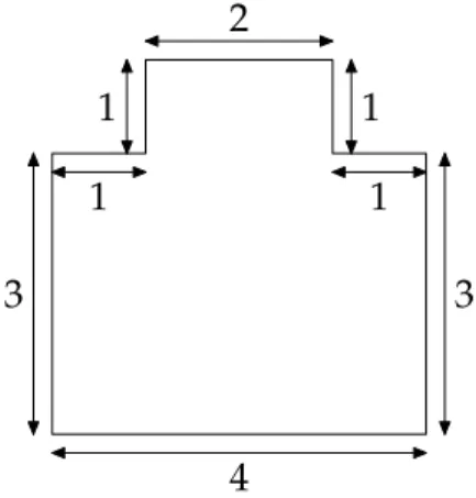
We deal with the 2 dimensional domain seen in Figure 1
4 3 1 1 2 1 1 3
First, we estimate the first eigenvalue λ2Dof 124 using the pdetool
pack-age from Matlab. In Table 1, we give the estimates of λ2D as a function of
the number of times we refine the mesh. Thus, its seems that the real value of λ2D is close to −0.740. The order of the second eigenvalue is −1.75.
# of nodes 180 670 2590 10200 40400 160940
−λ2D 0.7578 0.74532 0.74415 0.74021 0.73975 0.73958
Table 1: Estimate by Matlab/pdetool in function of the refinement of the mesh
4.2
The empirical distribution function of the first exit
time by Monte Carlo methods
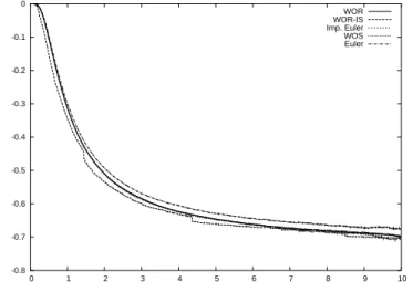
We have considered the simulation of the function F (t) using the different schemes described in Section 2 with 1.000.000 particles, excepted for the WOR-IS where 100.000.000 particles were used (see Section 2.4 for an ex-planation). For the Euler scheme, we use a time step ∆t of 10−3. For the walk on spheres, the absorption boundary layer is ε = 10−3. For the WOR and WOR-IS, we use only the two rectangles [0, 4] × [0, 3] and [1, 3] × [0, 4] (the lower left corner is at (0, 0)). The computation times are presented in Section 4.5. -0.8 -0.7 -0.6 -0.5 -0.4 -0.3 -0.2 -0.1 0 0 1 2 3 4 5 6 7 8 9 10 WOR WOR-IS Imp. Euler WOS Euler
Figure 2: t−1log(1 − FN(t)) for the different schemes
In Figure 2, we have drawn GN(t) = t−1log(1 − FN(t)) where the starting point is (2, 2). All the schemes give a function GN decreasing to a value
which is around −0.7 at t = 10, except for the naive Euler scheme for which it is around −0.67. For the WOR-IS, we have tested different strategies to force the process to stay longer times in the domain, but none were very successful. In addition, we see that the curves are perturbed by numerical artifacts.
Yet for large times, that is t > 7.0, the behavior becomes quite erratic, since it corresponds to the simulation of rare events. We cannot expect to obtain an accurate estimate of λ2D this way.
4.3
Estimation by the interpolation method
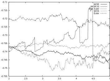
We then use the interpolation method of Section 3.2, with t2 − t1 = 4 and
we show in Figure 3 the values of λS
1(t1, t2) for t1 ∈ [2, 5]. -0.755 -0.75 -0.745 -0.74 -0.735 -0.73 -0.725 -0.72 -0.715 -0.71 2 2.5 3 3.5 4 4.5 5 WOR WOR-IS Imp. Euler WOS Euler
Figure 3: The estimator λIn(t
1, t1+ 4) for the different schemes
We obtain more accurate estimators than with the previous method. We still observe a deterioration when t1 is too large for all the schemes. However,
the naive Euler scheme gives an overestimated value of λ2D, which can be
easily explained by its nature. We no longer consider this scheme in the following.
If we look for the value of λIn(t
1, t1+4) with t1 in some particular intervals,
e.g. t1 ∈ [2, 3], we can see that all the estimators are very close to −0.74
and this for all the remaining schemes. We now turn to more quantitative results.
4.4
Optimization of the estimators
To estimate λ2D, we are free to choose the range of time t for F (t). The idea
is then to consider an estimator λ(i)2D of λ2D using the data on an interval
[ai, bi] for a large choice of ai and bi. We perform a statistical analysis of the set of the λ(i)2D for which a quality criterion is satisfied.
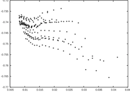
We first use the confidence interval techniques of Section 3.2 after having remarked on Figure 3 that all the estimators λIn(t
1, t1 + 4) are contained in
a narrow band for t1 ∈ [2, 5]. We now compute all the possible estimators
λIn(t
1, t2) and their relative confidence intervals, where t1, t2 are chosen on a
grid ηZ with η = 1/10, t1 ≥ 2, t2 ≤ 8 and t2− t1 ≥ 2. We only keep the
fraction of these estimators for which the length of the confidence interval is small. Indeed, we have to find a balance in the length `90%(t1, t2) of the
confidence interval at 90% given by (1) between the term 1/(t2 − t1) which
shall be small and the term s1/p1+s2/p2that increases when t1or t2increases.
We plot λIn(t
1, t2) against `90%(t1, t2) and we remark that the quality of the
approximation decreases when `90%(t1, t2) increases.
-0.77 -0.765 -0.76 -0.755 -0.75 -0.745 -0.74 -0.735 -0.73 0.005 0.01 0.015 0.02 0.025 0.03 0.035 0.04 0.045 Figure 4: λIn(t
1, t2) in function of `90%(t1, t2) for the improved Euler scheme
We also note that the smallest values of `90%(t1, t2) are obtained when t1
is close to 2 and t2 close to 5.
We now present our results on Table 2 using classical statistical estimators for the λIn(t
Method Improved Euler WOS WOR WOS-IS Min. −0.7423 −0.7385 −0.7398 −0.7537 1st Qu. −0.7403 −0.7378 −0.7376 −0.7456 Median −0.7392 −0.7373 −0.7373 −0.7393 Mean −0.7391 −0.7372 −0.7374 −0.7404 3rd Qu. −0.7377 −0.7368 −0.7369 −0.7364 Max −0.7365 −0.7351 −0.7361 −0.7268
Table 2: Study of the estimators λIn(t
1, t2) by keeping the 10% having the
smallest value of `90%(t1, t2)
If we look at the median or the mean of the estimators λIn(t
1, t2), we can
reach an accuracy of at least 3 · 10−3. All the schemes give an analogous accuracy.
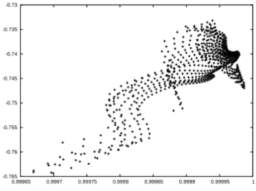
We now turn to the least squares method, by replacing our criterion on the length of the confidence interval by a criterion based on the correlation coef-ficient R. This coefcoef-ficient measures the validity of the linear approximation. We denote by λLS(t
1, t2) the estimator of λLS(t1, t2) giving the slope of the
linear regression of GN(t) with t ∈ [t1, t2]. We select the estimators λLS(t1, t2)
for which R2 is greater than 0.99997. We also plot λLS(t
1, t2) against the
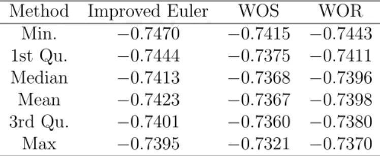
co-efficient R2. We now present our results on λLS(t
1, t2) in Table 3 as we did previously for λIn(t 1, t2). -0.765 -0.76 -0.755 -0.75 -0.745 -0.74 -0.735 -0.73 0.99965 0.9997 0.99975 0.9998 0.99985 0.9999 0.99995 1 Figure 5: λLS(t
Method Improved Euler WOS WOR Min. −0.7470 −0.7415 −0.7443 1st Qu. −0.7444 −0.7375 −0.7411 Median −0.7413 −0.7368 −0.7396 Mean −0.7423 −0.7367 −0.7398 3rd Qu. −0.7401 −0.7360 −0.7380 Max −0.7395 −0.7321 −0.7370
Table 3: Study of the estimators λLS(t
1, t2) for R2 > 0.99997
Once again, we obtained a good accuracy on the first eigenvalue λ2D (at
least 3 · 10−3). However, for the WOR-IS, this criterion is less robust and we have obtained an accuracy 3 · 10−2 and thus we do not include the results in Table 3.
4.5
Computation times
Although the schemes give close estimated values of λ2D, their relative
com-putation times differ largely and may be function of the choice of some pa-rameters, as seen in Table 4. The simulations were done on a bi-processors DEC 700MHz.
Scheme Parameter name Parameter Time (s) Avg. # steps
Euler time step ∆t 10−2
10−3
210 1400
200 2000
WOS boundary layer ε 10−3
10−4 80 85 13 16 WOR — — 700 1.5 WOR-IS — — 16 2.1
Table 4: Computations times with N = 1.000.000 for all the methods
We compare first the average number of steps of each of the methods. The WOR and WOR-IS take around two steps to reach the boundary. The WOS takes around ten times more steps using a boundary layer ε = 10−4. This number of steps increases slowly like a O(| log(ε)|) as ε goes to zero. The Euler scheme with ∆t = 10−2 takes ten times more steps than the WOS. This number of steps increases linearly with ∆t (if ∆t is divided by 10 the number of steps is ten times greater). If we now look at the CPU times, the WOR-IS is really the fastest method as its average number of steps is 2 and that it
requires the simulation of fairly simple random variables. Unfortunately, this method increases somehow the variance of the simulations. A lot more sam-ples are required to make it as accurate as the other methods. The simulation times of the WOR and of the Euler scheme are comparable. The first one requires only 1.5 steps but the simulation of complex random variables. The second one requires many steps but the simulation of very simple Gaussian random variables. A good arrangement between these methods appears to be the WOS. The average number of steps is small and the random variables to simulate are not too complex.
4.6
Preliminary conclusions
Our approach is efficient on this test case. However, among the schemes we have tested, the naive Euler scheme shall be discarded. Our statistical study gives an approximation of λ2D with an accuracy of order 3 · 10−3, which
corresponds to what can be expected from the replacement of F (t) by an empirical distribution function, due to the Kolmogorov-Smirnov theorem.
In practice, we recommend the two following methods: (a) We look graphically at either λIn(t
1, t1+ τ ) for a given τ and t1 in the
range of the obtained values and we then determine a range of times for which the oscillations around a constant value are small enough. We may use either the least squares method or the interpolation method. (b) We use the least squares methods to estimate λLS(t
1, t2) for a large
number of values of t1 < t2 with t2 − t1 ≥ τ for an arbitrary τ , and
keep the values of λLS(t
1, t2) for which the coefficient R2is large enough.
5
More complex problems
5.1
A three dimensional problem
We now consider the extension of our 2D problem where we add a third di-mension z ∈ [0, 4]. We could treat as well more complex three didi-mensional domains but we use this problem as its main eigenvalue can be simply com-puted. By a separation of variables argument, we have λ2D− π
2
32 ' −1.048.
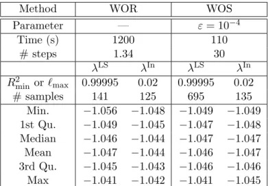
In Table 5, we use confidence intervals and least squares approximations for intervals [t1, t2] contained in [2, 8] with t2− t1 ≥ 2 and a step of 0.1 for t1
Method WOR WOS Parameter — ε = 10−4 Time (s) 1200 110 # steps 1.34 30 λLS λIn λLS λIn R2 min or `max 0.99995 0.02 0.99995 0.02 # samples 141 125 695 135 Min. −1.056 −1.048 −1.049 −1.049 1st Qu. −1.049 −1.045 −1.047 −1.048 Median −1.046 −1.044 −1.047 −1.047 Mean −1.047 −1.044 −1.046 −1.047 3rd Qu. −1.045 −1.043 −1.046 −1.046 Max −1.041 −1.042 −1.041 −1.045
Table 5: Study of the estimators λIn(t
1, t2) for `90%(t1, t2) ≤ `max and
λLS(t
1, t2) for R2 ≥ R2min with N = 1.000.000 particles.
We focus on this example on the WOR ans WOS methods. For the WOS, we need to simulate the uniform law on the unit sphere. This density writes
f (θ, ϕ) = 1
2sin(θ)1[0,π)(θ) 1
2π1[0,2π)(ϕ). The three Cartesian coordinates are
x = sin(θ) sin(ϕ), y = sin(θ) cos(ϕ), z = cos(θ)
where the density of θ is 1
2sin(θ)1[0,π)(θ) and where ϕ is uniform on [0, 2π).
The simulation of θ is achieved using the standard method by 2 arcsin(√U)
where U is uniform on [0, 1). The distribution function of the exit time from the unit ball is obtained via Monte Carlo simulations.
We note that once again we obtain an accuracy of about three digits on the principal eigenvalue using either the WOR or the WOS method. The two statistical methods lead to very similar approximations. If we look at the CPU times, we observe that they increase only linearly with the dimension of the problem.
5.2
A five dimensional problem
We now take some more examples in dimension 5 to emphasize that our method is not very sensitive to the dimensional effect. Similarly to the 3D case, we consider the Dirichlet problem on the domain
Using again a separation of variables, the first eigenvalue λ5D is λ2D −
3π2/32 ' −1.665, if λ
2D is approximated by −0.740.
In Table 6, we use confidence intervals and least squares approximations for intervals [t1, t2] contained in [2, 6] with t2− t1 ≥ 2 and a step of 0.1.
Method WOR Imp. Euler Imp. Euler
Parameter — ∆t = 10−2 ∆t = 6 · 10−3 Time (s) 2000 300 440 # steps 1.23 123 200 λLS λIn λLS λIn λLS λIn R2 min or `max 0.99995 0.06 0.9999 0.06 0.9999 0.06 # samples 20 56 140 62 90 64 Min. −1.666 −1.682 −1.692 −1.677 −1.667 −1.673 1st Qu. −1.663 −1.677 −1.676 −1.671 −1.663 −1.666 Median −1.662 −1.672 −1.671 −1.668 −1.658 −1.657 Mean −1.661 −1.672 −1.671 −1.667 −1.658 −1.658 3rd Qu. −1.659 −1.666 −1.667 −1.665 −1.653 −1.650 Max −1.654 −1.662 −1.651 −1.657 −1.646 −1.645
Table 6: Study of the estimators λIn(t
1, t2) for `90%(t1, t2) ≤ `max and
λLS(t
1, t2) for R2 ≥ R2min with N = 1.000.000 particles.
As the WOS is not so easy to implement in this case, we now use the WOR and the improved Euler scheme in the simulations. We still obtain in less than 10 minutes of CPU a good accuracy of about 3 · 10−3 on the eigenvalue for a problem which is very difficult to solve by means of deterministic methods. The CPU times of the WOR still increases linearly. It seems sufficient to use a discretization parameter of ∆t = 10−2 for the Euler Scheme to reach this accuracy. We can certainly recommend this method for such difficult problems as it is very easy to implement.
6
Conclusion
We have presented and tested a Monte Carlo method to compute the first eigenvalue λ1 of the Laplace operator with Dirichlet boundary condition.
This method is based on the numerical computation of the speed of absorp-tion of the Brownian moabsorp-tion by the boundary of the domain. It requires a good approximation of the law of the exit time of the Brownian motion by means of various schemes and also accurate estimators of λ1 seen as a
We have to note that the estimators of λ1 are very sensitive to the quality
of the empirical distribution function of the exit time. In our least squares method, we have however developed a test based on the coefficient R2, which
appears to be robust in all our experiments. The accuracy is anyhow limited by the speed of convergence given by the Kolmogorov-Smirnov theorem.
The WOR-IS is not efficient in our case, while the naive Euler scheme overestimates λ and is also to be rejected for this purpose. Yet some variants of the Euler scheme provide much more better estimates, while remaining easy to set up. The WOS is the fastest method there, but may be difficult to set up in high dimension. For polytopes, the WOR provides a good approxi-mation of λ1 but takes longer time in high dimension, and is more difficult to
implement. Note that however partial tabulations of some random variables and a better use of the WOR-IS should provide very efficient methods.
On all our test cases, from dimension 2 to 5, we have obtained in no more than 10 min an accuracy of about 3 digits on the eigenvalue λ1 using
1.000.000 particles. Of course, in our test cases, the geometry of the domain was rather simple, but the different methods can be combined to deal with more complex geometries. We can also add that our method is even more valuable in dimension greater than 3, where deterministic methods are lim-ited by the difficulty of generating a mesh and the size of the matrix to invert. In all our methods, the computation time increases linearly with the dimen-sion, and none requires the construction of a mesh. Besides, this method can be extended to deal with a general second-order elliptic operator. The com-putation of λ1 could also be a good test to evaluate the efficiency of diffusion
approximations.
References
[1] A. Borodin and P. Salminen, Handbook of Brownian motion: facts
and formulae. Birkh¨auser, 1996. 4
[2] D. Brockway, P. Soran and P. Whalen. Monte Carlo eigenvalue calculation, in Monte-Carlo methods and applications in neutronics,
photonics and statistical physics. R. Alcouffe et al. (Eds), 378–384,
Springer-Verlag, 1985. 8
[3] F. M. Buchmann. Simulations of stopped diffusions, J. Comput. Phys. 202, no. 2, 446–462, 2005. 4
[4] F. Campillo and A. Lejay. A Monte Carlo method without grid for a fractured porous domain model, Monte Carlo Methods Appl., 8, no. 2, 129–148, 2002. 5
[5] M. Deaconu and A. Lejay. A random walk on rectangles algorithm.
Methodol. Comput. Appl. Probab., 8, no. 1, 135–151, 2006. 5, 6
[6] M. Deaconu and A. Lejay. Simulation of a diffusion process using the importance sampling paradigm. In preparation, 2005. 6
[7] M. Freidlin. Functional Integration and Partial Differential Equations. Princeton University Press, 1985. 3
[8] A. Friedman. Stochastic Differential Equations and Applications,
Vol-ume 2, Academic Press, 1976. 3
[9] E. Gobet. Weak approximations of killed diffusions using Euler schemes. Stoch. Process. Appl., 87, no. 2, pp 167-197, 2000. 4
[10] E. Gobet. Euler schemes and half-space approximations for the sim-ulation of diffusion in a domain, ESAIM Probability and Statistics, 5, 261–297, 2001. 4
[11] E. Gobet and S. Menozzi. Exact approximation rate of killed hy-poelliptic diffusions using the discrete Euler scheme, Stochastic Process.
Appl., 112, no. 2, 201–223, 2004. 4
[12] N. Golyandina. Convergence rate for spherical processes with shifted centres. Monte Carlo Methods Appl. 10, no. 3–4, 287–296, 2004. 5 [13] Y. Kifer. Random perturbations of dynamical systems. Progress in
Probability and Statistics, 16. Birkh¨auser, 1988. 3, 8
[14] P. Kloeden and E. Platen. Numerical solution of stochastic
differ-ential equations. Applications of Mathematics, Springer-Verlag, Berlin,
1992. 3
[15] B. Lapeyre, E. Pardoux and R. Sentis. M´ethodes de Monte-Carlo
pour les ´equations de transport et de diffusion. Springer-Verlag, 1998. 2
[16] S. Maire. R´eduction de variance pour l’int´egration num´erique et pour
le calcul critique en transport neutronique, Phd thesis, Universit´e de
[17] S. Maire and D. Talay. On a Monte Carlo method for neutron transport criticality computations. IMA J. Numer. Anal., to appear, DOI:10.1093/imanum/drl008, 2006. 2, 3, 9
[18] G. Milstein and M. Tretyakov. Simulation of a space-time bounded diffusion. Ann. Appl. Probab., 9, no. 3, 732–779, 1999. 5
[19] R. G. Pinsky. Positive harmonic functions and diffusion. Cambridge Studies in Advanced Mathematics, 45. Cambridge University Press, 1995. 3, 7
[20] K. Sabelfeld. Monte Carlo methods in boundary value problems. Springer, 1991. 4
[21] G. Shorack and J. Wellner. Empirical processes with applications
to statistics. Wiley Series in Probability and Mathematical Statistics: