HAL Id: hal-00617464
https://hal.archives-ouvertes.fr/hal-00617464
Submitted on 29 Aug 2011
HAL is a multi-disciplinary open access archive for the deposit and dissemination of sci-entific research documents, whether they are pub-lished or not. The documents may come from
L’archive ouverte pluridisciplinaire HAL, est destinée au dépôt et à la diffusion de documents scientifiques de niveau recherche, publiés ou non, émanant des établissements d’enseignement et de
Numerical investigation of a three-dimensional four field
model for collisionless magnetic reconnection
D. Grasso, D. Borgogno, Emanuele Tassi
To cite this version:
D. Grasso, D. Borgogno, Emanuele Tassi. Numerical investigation of a three-dimensional four field model for collisionless magnetic reconnection. Communications in Nonlinear Science and Numerical Simulation, Elsevier, 2012, 17, pp.2085. �hal-00617464�
Numerical investigation of a three-dimensional four field
model for collisionless magnetic reconnection
D. Grasso1
, D. Borgogno2
, E. Tassi3
1. CNR Consiglio Nazionale delle Ricerche, Istituto dei Sistemi Complessi, Dipartimento
di Energetica, Politecnico di Torino Corso Duca degli Abruzzi 24, I-10129 Torino, Italy
2. Dipartimento di Energetica, Politecnico di Torino, Corso Duca degli Abruzzi 24, 10129
Torino, Italy
3.Centre de Physique Th´eorique, CNRS – Aix-Marseille Universit´es, Campus de Luminy,
case 907, F-13288 Marseille cedex 09, France
Abstract
In this paper we present the numerical investigation of a three-dimensional four field model for magnetic reconnection in collisionless regimes. The model describes the evolution of the magnetic flux and vorticity together with the perturbations of the parallel magnetic and velocity fields. We explored the different behavior of vorticity and current density structures in low and high β regimes, β being the ratio between the plasma and magnetic pressure. A detailed analysis of the velocity field advecting the relevant physical quanti-ties is presented. We show that, as the reconnection process evolves, velocity layers develop and become more and more localized. The shear of these layers increases with time ending up with the occurrence of secondary instabilities of the Kelvin-Helmholtz type. We also show how the β parameter influences the different evolution of the current density structures, that preserve for longer time a laminar behavior at smaller β values. A qualitative explana-tion of the structures formaexplana-tion on the different z-secexplana-tions is also presented.
Key words: Nonlinear dynamics, plasma instabilities, fluid instabilities, numerical simulations
1. Introduction
Magnetic reconnection is a fundamental process in highly conductive flu-ids and plasmas [1, 2]. It can be defined as a change in the topology of the magnetic field lines, which decouple their motion from the fluid one. It is
associated with a release of magnetic energy into heat, plasma kinetic energy and fast particle energy and it is characterized by the formation of current density sheets in the reconnection region along with strong velocity layers. The range of phenomena involving magnetic reconnection is very wide. It includes solar flares, geomagnetic substorms, interaction of the solar wind with the magnetopause, sawtooth oscillations and disruptions in laboratory plasma, such as in Tokamaks. One of the problems in magnetic reconnection is to identify the appropriate generalized Ohm’s law and the physical mech-anisms which cause the diffusion of the magnetic field through the plasma. In weakly collisional plasmas, such as the high temperature ones in Toka-maks, the inverse of the electron-ion collision frequency is larger than the relaxation time of internal sawtooth oscillations. This consideration made collisionless reconnection to become a frontier subject in the early ’90 [3, 4]. In this regime the typical length scale of the reconnection process is given by the collisionless skin depth, de. Although a kinetic approach should be
invoked in order to treat such collisionless regimes, in the presence of a strong guide field, fluid models, which offer a computational advantage, are often used. Many studies have been done in the framework of two-fluid models. In this context a description of the plasma behavior can be made considering a simpler two-field description [5] or a more sophisticated four-field description [6]. In particular, the two-field model in [5] has been extensively analyzed in the last decade both in two-dimensional and three-dimensional configu-rations [7, 8, 9, 10]. In this model the evolution of the magnetic flux and plasma stream function is followed assuming that variations of the magnetic field and of the plasma velocity, along the direction parallel to the guide field, are negligible. The fingerprint of this approach is the coupling between the evolution of the current density and vorticity fields, which evolve in ordered or turbulent structures depending on the value of the electron temperature, which enters the equation through the the ion sound Larmor radius ̺s [7, 9],
which is a further characteristic scale length of the phenomenon. For values of ̺s ≥ de the velocity layers,advecting the current density and vorticity,
evolve in ordered coherent structures aligned with the separatrix of the mag-netic island. On the other hand, for ̺s << de the velocity layers tend to
be aligned with the neutral line giving rise to strong shears that lead to the onset of secondary Kelvin-Helmholtz instabilities. This twofold picture has been also confirmed in three-dimensional configurations [10, 11]. When we allow the system to develop also magnetic and plasma velocity perturbations along the direction parallel to the guide field, by considering the four-field
model in [6], the picture becomes richer and a new scenario appears, where the evolutions of the current density and vorticity fields are no longer cou-pled. The crucial role in this change is played by the β parameter, expressing the ratio between the plasma and the magnetic field pressures. Indeed, when the low β limit is abandoned, the effects of the strong velocity shears that develop in the reconnection region, on one hand lead to a turbulent vorticity, but on the other hand they get suppressed in the evolution of the current density [11, 12].
Recently, an extension of this four-field model to three dimensions has also been derived [13]. The model belongs to the class of fluid models for plasma physics, for which a noncanonical Hamiltonian formulation is known. The origin of this class can be traced back to the seminal work of Morrison and Greene [14] on ideal magnetohydrodynamics. The class was subsequently enlarged to a great extent by Phil Morrison and co-workers over the years, with the discovery of Hamiltonian structures for several reduced fluid models. In this article we analyze this model by performing numerical simulations with the aim of investigating the evolution, and its dependence on β, of velocity and current density fields in a full 3D setting. In particular we address the question of understanding in what fields the secondary Kelvin-Helmholtz instability dominates and in what fields it is suppressed, and how such instability extends along the z direction. We also recall that the absence of an ignorable coordinate raises the problem of interpreting a dynamics which is much less constrained than the two-dimensional one[15, 10, 11]. In particular, the system no longer possesses the infinity of Casimir invariants which constrain the 2D case and in terms of which it is possible to explain the different structures observed in the current density and vorticity fields [5, 8, 16, 12]. Such explanation was indeed possible, due to the presence of advected scalar fields whose existence was related to the presence of an infinite number of Casimirs. The paper is organized as follows: in Sec. 2 we present the model equations; in Sec. 3 the simulation results are shown and discussed; in Sec. 4 we focus on the energy partition; conclusions are drawn in Sec. 5.
2. Model equations
Our investigation is based on the 3D four-field model for collisionless re-connection, described in Ref.[13]. Considering a Cartesian coordinate system (x, y, z), with the constant magnetic guide field directed along z, the model
equations are given by ∂(ψ − d2 e∇ 2 ⊥ψ) ∂t + [ϕ, ψ − d 2 e∇ 2 ⊥ψ] − dβ[ψ, Z] + ∂ϕ ∂z + dβ ∂Z ∂z = 0, (1) ∂Z ∂t + [ϕ, Z] − cβ[v, ψ] − dβ[∇ 2 ⊥ψ, ψ] − cβ ∂v ∂z − dβ ∂∇2 ⊥ψ ∂z = 0, (2) ∂∇2 ⊥ϕ ∂t + [ϕ, ∇ 2 ⊥ϕ] + [∇ 2 ⊥ψ, ψ] + ∂∇2 ⊥ψ ∂z = 0, (3) ∂v ∂t + [ϕ, v] − cβ[Z, ψ] − cβ ∂Z ∂z = 0, (4) where ψ is the poloidal magnetic flux function, ϕ is the E × B stream func-tion, Z is proportional to the parallel magnetic perturbation and v is the par-allel plasma velocity. The parameter de represents the electron skin depth,
whereas the other two parameters cβ and dβ are defined by cβ ≡pβ/(1 + β),
with β indicating the ratio between the plasma pressure and the toroidal mag-netic pressure, and by dβ ≡ dicβ, where diis the ion skin depth. The Poisson
bracket is defined by [f, g] = ˆz · (∇f × ∇g) for generic fields f and g, whereas the symbol ∇⊥ refers to the gradient perpendicular to ˆz. Equations (1)-(4)
are written in a dimensionless form, according to which, the time is normal-ized with respect to a characteristic Alfv`en time tA, lengths are normalized
with respect to a characteristic scale L and magnetic fields with respect to a characteristic value B. If such value is taken to be the amplitude B0 of the
toroidal guide field, then the following ordering applies:
ψ ∼ ϕ ∼ Z ∼ v ∼ ∂ ∂t ∼ ∂ ∂z ∼ ǫ ≡ Bp B0 ≪ 1, (5) ∂ ∂x ∼ ∂ ∂y ∼ 1, (6)
where Bp indicates a characteristic value for the poloidal magnetic field
(re-mark that this ordering differs from that of Ref. [13], in which a normalization based on Bp, instead of B0, was adopted).
Note that the Eqs. (1)-(4) are exact only at the order ǫ2
. Indeed, in their derivation, only the contributions up to order ǫ of the normalized magnetic field
B= ˆz + ∇ψ × ˆz + cβZ ˆz + O(ǫ 2
), (7)
have been used. A term −cβ
Rx
0 dx
′∂Z/∂z ˆx , which is of order ǫ2
, is required in order to have a divergence-free magnetic field, but it produces only higher
order corrections to (1)-(4).
By construction, the system (1)-(4) is Hamiltonian and conserves the total energy H = 1 2 Z D d3 x (d2 eJ 2 + |∇⊥ϕ| 2 + v2 + |∇⊥ψ| 2 + Z2 ), (8) where J = −∇2
⊥ψ is the parallel current density and D is the domain of
interest. The corresponding Poisson bracket has been provided in Ref. [13].
3. Numerical results
The equations (1)-(4) are integrated numerically by splitting all the fields in two parts: an equilibrium, independent on time, and an evolving pertur-bation. The perturbed component is advanced in time by an explicit, fourth order Adam-Bashforth scheme. The equations are solved in a three dimen-sional slab, with periodic boundary conditions along the y and z directions. Dirichlet conditions are applied at the edges of the x axis, imposing that all the perturbed fields go to zero. A compact finite difference [17] algorithm, suitable for non-equispaced grid, is used for the spatial operations along the x direction, while pseudo-spectral methods are adopted for the periodic di-rections. Numerical filters are introduced in order to control the numerical error propagation, which is a relevant issue in the absence of any dissipative effect, as in the problem we are considering. As described in [17], these fil-ters smooth out the small spatial scales below a chosen cutoff, while leaving unchanged the large scale dynamics on all the time evolution of the process. Finally, in order to address the three-dimensional problem, the code has been parallelized adopting the MPI libraries. We set up a numerical experiment of spontaneous, 3D, collisionless reconnection process in a static equilibrium configuration with
ψeq = − log cosh(x) and ϕeq = veq = Zeq= 0. (9)
The integration domain is defined by −Lx < x < Lx, −Ly < y < Ly and
−Lz < z < Lz, where Lx = 11.32, Ly = 4π, Lz = 64π. The choice of Lx
avoids any influence of boundary conditions imposed along the x direction on the reconnection dynamics. The value of Ly allow to consider the magnetic
reconnection instability induced by highly unstable modes, that in the two-dimensional limit fall in the so-called large ∆′ regime. It is accepted [3, 4, 18]
time scale. Finally, the choice of Lz >> Ly guarantees that kz = 2πn/Lz <
ky = 2πm/Ly for all the pairs of mode numbers (m, n) that develop during
the nonlinear evolution of the process, as imposed by the conditions (5)-(6). In order to take into account the 3D effects on the magnetic reconnection we perturbed the equilibrium (9) by introducing the following double helicity perturbation on the current density field
δJ(x, y, z) = ˆJ1(x) exp(iky1y + ikz1z) + ˆJ2(x) exp(iky2y − ikz2z). (10)
Here we considered the pairs of wave numbers (1, 1) and (1, −1), that corre-spond to the wave vectors components ky1 = 1/4, kz1= 1/64 and ky2 = 1/4,
kz2 = −1/64. These two helicities, that are both linearly unstable, have
resonant surfaces at xs1 = 0.06258 and xs2 = −0.06258. ˆJ1(x) and ˆJ2(x)
are functions localized within a width of the order de, around xs1 and xs2,
respectively. Their typical amplitude is of order 10−4. In order to properly
treat the small scale structures that typically generate in the collisionless regimes a mesh of nx = 801, ny = nz = 512 grid points has been adopted. In this paper we analyzed the influence of the 3D effects on the dynamics of the magnetic reconnection instability by considering two sets of the physical parameters appearing in eqs. (1)-(4). In both cases we have used de = 0.24
and dβ = 0.96, while cβ is varied, assuming the values cβ = 0.4 and cβ = 0.8.
This choice allows to address two regimes with different values of the ion skin depth di and of the ratio, β, between the plasma and the magnetic field
pres-sure. In particular, when cβ = 0.4, β = 0.19, while cβ = 0.8 gives β = 1.78,
which we refer to as a small and a high β regimes.
3.1. Qualitative aspects of the dynamics along the z direction
As shown in the framework of a 3D, two-field, dissipationless model ([15],[10], [11]), the nonlinear interaction between two initially imposed lin-early unstable helicities strongly affects the spatial distribution of the small scale structures where current density and vorticity fields are located. The shape of these patterns is the consequence of the interaction between the current layers associated to the island chains corresponding to the imposed helicities. According to the 2D results [7], in the collisionless cases when ̺s 6= 0 the current density field exhibits a cross-shape structure distributed
along the separatrices of the magnetic islands, and is strongly peaked at the corresponding X points. For a single helicity with (ky, kz) wave vector, the
z following the lines with slope kz/ky, while the value of the x coordinate
does not depend on z. This remains valid also in presence of more than one helicity, at least at the very early stages of the nonlinear evolution. In the early phase, indeed, each helicity is characterized by a given number, depending on ky, of thin current density channels with a characteristic
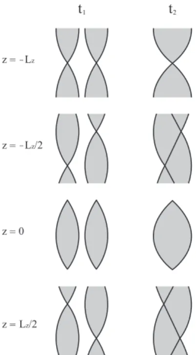
spa-tial orientation. Similarly to electric wires, the current density channels of various helicities interact among each other by means of attracting forces whose strength depends on their geometry. In particular, the maximum of the attraction is localized on the z = const sections where the centers of the current density channels, localized at the X-points of the corresponding magnetic islands, have the same y coordinates. On these sections the inter-action leads to the merging of the current channels. An opposite scenario characterizes the z = const planes where the X and O-points of the magnetic islands with different helicities face each other. Due to the fact that negative minimum current density values lie on the O points, very small attracting or even repulsive interactions act on the maximum current density peaks, as it is the case when two electric wires with currents flowing in opposite directions, face each other. Fig. 1 sketches this behavior for a double helicity case with poloidal and toroidal mode number m = 1, n = 1 and m = 1, n = −1. The figure shows the current density distribution on four z = const sections at the times t1 and t2, that correspond to the very beginning and the advanced
phases of the nonlinear evolution of the process. In the planes z = −Lz and
z = 0, where the X points of the structures have the same y coordinate, the current layers experience the maximum attraction and merge by gener-ating a single X point pattern at t = t2. On such planes, the dynamics is
quite similar to that observed in the single-helicity case. On the contrary, on the planes z = Lz/2 and z = −Lz/2, where the maximum current
den-sity of an island chain faces the minimum of the second chain, current layers merge by generating a new spatial distribution where two X-points are still present. The above described situations refer to the two extreme cases that can take place. Through the z = const planes, lying between those described above, the dynamics varies continuously with z, with a force between the current layers, which depends on the relative shift between the positions of the X-points along the y direction.
3.2. Interpretation of the numerical simulations
Due to the high value of dβ, the early stages of the nonlinear evolution of
We define here the end of the linear phase by the time in which the growth of the two initially imposed modes, deviates from the exponential one, which they would have when considered separately. In this early nonlinear phase of the evolution, the contribution of the terms proportional to cβ is almost
negligible with respect to the Poisson brackets involving dβ. Since, in this
limit, the parallel magnetic field perturbation Z becomes proportional to the vorticity U , the equations for F = ψ − d2
e∇ 2
⊥ψ and for U decouple from the
equations for Z and v and reduce to the two field limit of the model (1)-(4), described in [15], where ρs = dβ [16]. According to the two field model
results [11], also in this case the current density and vorticity field concen-trate in analogous structures characterized by thin and sharp layers on all the z = const sections. Due to the proportionality with U , similar patterns develop also in Z, while the parallel velocity component v is characterized by large scale cell structures similarly to v⊥ = |∇⊥ϕ|, the field which it is
mainly transported by. This behavior is illustrated in figure 2, where the contour plots of U , Z, J and v are plotted on the particular plane z = 0 at t = 90τA for the cβ = 0.8 case.
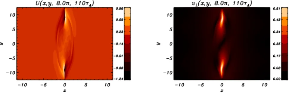
When the influence of cβ effects becomes important, at the later stages of
the process, the vorticity layers tend to broaden, starting from the z = const sections where the X points of the linear magnetic islands associated with the different helicities have similar y coordinate. This leads to the formation of new vorticity structures, localized around the x=0 axis for the particular choice of symmetric initial conditions we assumed, and, as a consequence, of highly localized, bar shaped, perpendicular velocity layers similar to jets as shown in figure 3. As already pointed out in Ref. [13], when the influence of a finite β is not negligible, the structures of U and Z eventually differ. On the other hand, from Eqs. (2) and (3), one sees that in the limit cβ → 0
(but with finite dβ) the relation Z = dβU satisfies the system, if the initial
conditions on Z and U are the same, which is the case here. This explains the similarity in the structures of Z and U for negligible β.
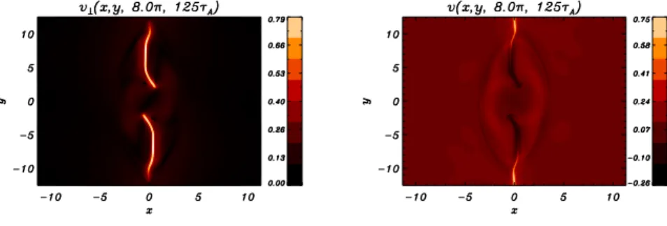
The amplitude of the perpendicular velocity tends to become stronger as the magnetic reconnection develops. In the advanced nonlinear phase it provides the dominant contribution both in the equations of the vorticity and the par-allel velocity fields. U and v are simply transported along the perpendicular velocity and as a consequence they assume the same spatial distribution of v⊥. On the other hand, due to the value of dβ we considered, the time
evolu-tion of J and Z continues to be dominated by the nonlinear terms involving the perpendicular component of the magnetic field, dβ[ψ, Z] and dβ[∇
2 ⊥ψ, ψ]
respectively. In figure 4 the intense jets appearing on the z = 0 section for the perpendicular and parallel velocities are shown together with the more ordered structures characterizing Z and J.
The fronts of both the parallel and perpendicular velocity jets tend to move towards the center of the computational box starting from the boundary sur-faces y = ±4π. Approaching the y = 0 plane, the tops of the jets roll up and assume a “mushroom cap” shape which makes the velocity layers very similar to the “finger” like structures typical of the hydrodynamic Rayleigh-Taylor instability. This suggests the fluid like behavior of the system in these structures. Despite the magnetic field line stochasticity which characterizes the 3D settings we treat here, in fact, magnetic field components parallel to the jets are practically zero, which makes the contribution of the Poisson brackets [∇2
⊥ψ, ψ] and [Z, ψ] locally negligible and reduces the U and v
equa-tions to purely fluid advection equaequa-tions. This justifies the occurrence, at later times, when the width of the jets is of the order of de and the velocity
is comparable to vA, of a Kelvin-Helmholtz like secondary instability which
is responsible for the break of the velocity patterns.
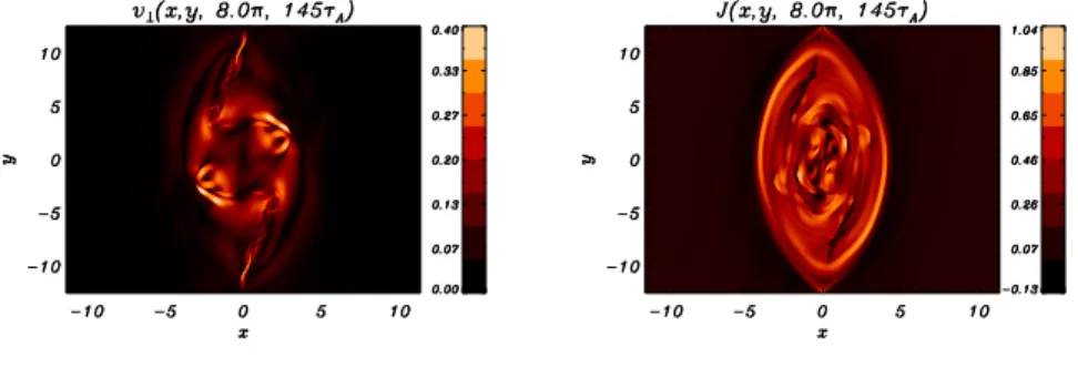
At this stage cβ effects appear also on J and Z fields producing a
turbu-lent redistribution of the patterns in the regions where v⊥ and v are picked,
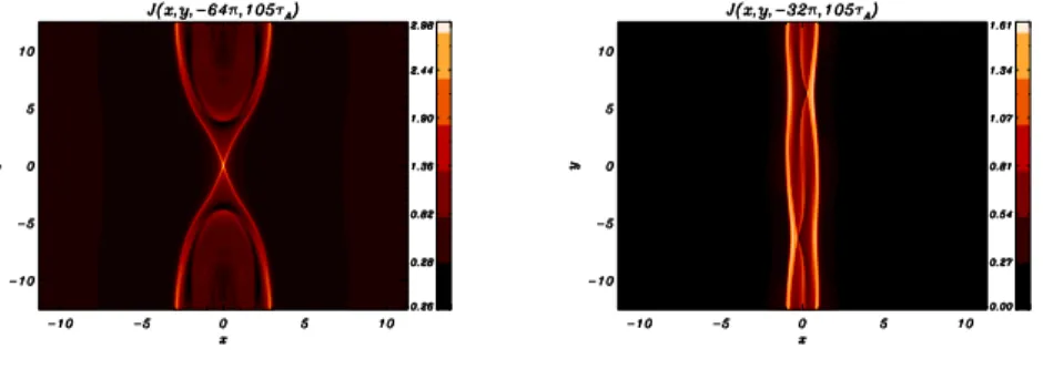
which coexists with the laminar filaments concentrated at the boundaries of the reconnection area. This behavior is clearly illustrated in fig. 5, where the perpendicular velocity and current density are shown on the z = 8π section at the latest stage of the process for the case cβ = 0.8.
On the x − y planes with a larger distance between the y coordinates of the linear magnetic island X-points the contribution of cβ remains rather small
all along the reconnection process. On these sections, in fact, the nonlinear coupling between the current density structures do not allow the formation of the intense and extremely localized velocity layers described above, as il-lustrated in fig. 6. Here a comparison of the merging of the current density layers is shown on two different planes. On the left is the contour plot as it appears at z = −64π and on the right as it appears at z = 32π plane. These planes correspond to the first and second sketch of fig. 1 respectively. We can see that the current density layers tend to broaden and their intensity is reduced as far as we consider z-planes where the distance between the y coordinates of the X-points, corresponding to the two initially imposed he-licities, increases. Because of the dominant terms depending on dβ, the U , J
and Z fields exhibit analogous patterns, while v⊥ and v are characterized by
It is also interesting to comment on the difference between a small and a high β regimes, which we consider as represented by the cβ = 0.4 and cβ = 0.8
cases, respectively. In particular, in the high-β regime, one has dβ ≈ di
and this parameter measures the strength of the Hall term in the equations governing the magnetic dynamics. In the 2D limit, the model becomes then identical to the Hall MHD model investigated in Ref. [19], apart from the dif-ference in the mechanism breaking the frozen-in condition. The comparison between the cβ = 0.4 and cβ = 0.8 cases confirms that also in 3D geometry
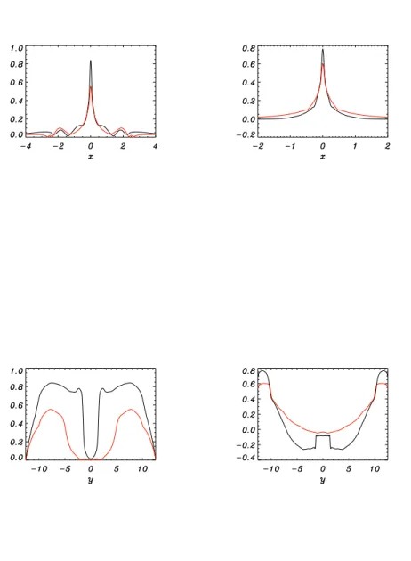
larger values of the β parameter accelerate the formation of the fluid jets, whose occurrence happens at earlier stages of the reconnection process. Par-allel and perpendicular velocities inside the layers are typically smaller in the lower β case, for comparable extensions of the reconnection region on a given z = const section. This difference is highlighted in fig. 7, where the profiles of the velocity fields v⊥ and v are shown on the section z = 0 for the two
different values of cβ mentioned above. In particular, on the first row v⊥(left
frame) and v (right frame) are plotted as function of x, in the limited range −4 < x < 4 and −2 < x < 2 respectively, at the y coordinate corresponding to their maximum. We see that, when considered at times which correspond to the same phase of the evolution of the reconnection process in the two cases, the velocity fields are smaller by a factor of order two in the lower cβ limit, drawn in red. This characteristic is seen also in the second row of
fig. 7, where the velocity fields are plotted as function of y at x = 0, where the fluids jets are located. Here, we can also appreciate that the extension of the fluid jets, which start at the boundaries y = ±4π for both cases, is shorter when cβ = 0.4. In this case (red lines) the jets end at y = ±5 while
for cβ = 0.8 (black lines) they end at y = ±1 approximately. This is due to
the fact that the jets formation started earlier for the cβ = 0.8. As it will
be seen in the next section, greater outflow speeds in the parallel direction, at high β, can be ascribed to a transfer of energy, mediated by the Lorentz force, from the magnetic to the kinetic form. The amount of transferred energy is indeed proportional to cβ. Therefore one can expect a greater
ac-celeration at higher β. We remark also that, because the Hamiltonian (8) is independent on β, the total energy available in the small and high β case is the same. Therefore, increase of the parallel kinetic energy with β is a pure consequence of the dynamical transfer and is not influenced by differences in the total energy of the system. Finally, we notice that, as a consequence of having less steep velocity layers for small β, in the latter case the Kelvin-Helmholtz destabilization of the fluid jets is delayed, making its influence on
the density current and parallel magnetic field perturbation rather smooth.
4. Energy considerations
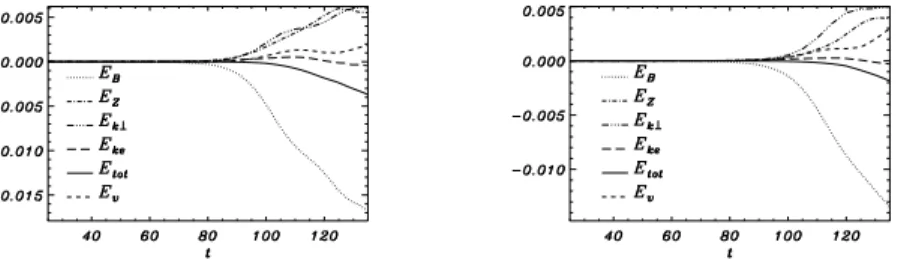
Because the model under consideration is a Hamiltonian system, the total energy (8) should be preserved during the dynamics. It is therefore impor-tant to verify that the decay of H, due to numerical dissipation, remains negligible. From Fig. 8 it is possible to see that, at the latest time of the simulation, the drop in the total energy for both the cases reported is less than 4 h. We remark also that, during most of the simulations, the velocity at which the magnetic energy decreases is much larger than that at which the total energy dissipates. This reassures us of the fact that the magnetic energy loss is due to a genuine reconnection (or also ideal) process and not to numerical dissipation.
In addition to remarks concerning the reliability of the simulations, the anal-ysis of the time evolution of the different forms of energy is also suitable for physical considerations. Fig. 8 shows how, evidently, the perpendicu-lar magnetic energy is converted into various forms during the reconnection process. In order to better understand the mechanisms of transfer of energy, it is useful to consider the following relations, which can be easily obtained from the model equations (1)-(4):
d dt 1 2 Z d3 x|∇⊥ϕ| 2 = Z d3 xJ(B · ∇)ϕ + O(ǫ4 ), (11) d dt 1 2 Z d3 xv2 = cβ Z d3 xv(B · ∇)Z + O(ǫ4 ), (12) d dt 1 2 Z d3 x(|∇⊥ψ| 2 + d2 eJ 2 ) = − Z d3 xJ(B · ∇)ϕ −dβ Z d3 xJ(B · ∇)Z + O(ǫ4 ), (13) d dt 1 2 Z d3 xZ2 = −cβ Z d3 xv(B · ∇)Z +dβ Z d3 xJ(B · ∇)Z + O(ǫ4 ). (14)
In order to obtain compact and physically more meaningful expressions, we express the right-hand sides of (11)-(14) in terms of the magnetic field B, instead of ψ and Z. As a consequence, by virtue of what was specified
in Sec.2, the resulting expressions are exact only at the leading order and corrections of order ǫ4
are required. Of course, giving up B in favor of ψ and Z, yields the relations whose sum gives the exact conservation of the Hamiltonian H. Note also that all the leading order terms on the right-hand sides of (11)−(14) possess the common formR d3
xf (B·∇)g, for generic fields f and g. Mechanisms that produce the transfer of energy from one form to another, can then become inefficient if some fields have a weak variation along the magnetic field lines.
From Eqs. (11) and (13), we see that the mechanism that acts as a source for perpendicular kinetic energy, is a sink for the energy of the poloidal magnetic field and of the parallel current. The rise of Ekperp observed in
Fig. 8, then implies a drop in EB+ Eke. The growth of the parallel kinetic
energy, on the other hand, is possible only at finite β, in which case the parallel Lorentz accelerates the fluid. This mechanism acts also as a sink for the parallel magnetic energy. Note that, in Fig. 8, for the smaller cβ case,
there is a competition between the conversion of magnetic energy into parallel magnetic energy and perpendicular kinetic energy, which lasts until around t = 125 i.e. well into the nonlinear phase, when EZ reaches its maximum
and then drops. At the same time, an increase in Ev is observed. On the
other hand, for the larger cβ case, the conversion into perpendicular plasma
kinetic energy, is dominant from the beginning of the nonlinear phase. We notice also that the form of energies that grow the most in the last phase of the simulations, i.e. Ev and Ekperp, are those determined by the fields, v and
|∇⊥ϕ|, respectively, which exhibit the secondary instability.
5. Conclusions
In this paper we analyzed a three-dimensional model for collisionless re-connection, which takes into account magnetic and velocity perturbations along the guide field direction. On the basis of previous two-dimensional studies we were interested in exploring in a 3D context the different behavior of the current density and vorticity structures. To this aim, we carried out a detailed analysis of the plasma velocity fields, which play a key role in the current density and vorticity dynamics. In the presence of high values of the dβ parameter, we found that, during the early stages of the nonlinear
phase, the perpendicular and parallel velocities on the z = const sections are characterized by large scale cell structures. The other fields J, U and Z, on the other hand, develop thinner spatial patterns similar to the case
β = 0. Following the evolution process, we observe that the perpendicular velocity tends to form highly localized patterns, aligned along the x = 0 line, on some peculiar z = const sections, which depend on the particular choice of the initial perturbation. These patterns are then recaptured also in the parallel velocity and vorticity fields, while, due to the high value of the dβ parameter chosen for this analysis, the evolution of the current density
and of the Z field, is dominated by the contribution of the Poisson brackets involving the magnetic flux.
At the end of the reconnection process both the perpendicular and par-allel velocity layers have become so localized and intense that they develop secondary instabilities of the Kelvin-Helmholtz type. In connection with this we find that the larger cβ, the sooner these instabilities develop.
The increase of the velocities fields and the occurrence of secondary in-stabilities influence also the energy distribution, favoring the conversion of the perpendicular magnetic energy into perpendicular and parallel kinetic energy rather than into parallel magnetic energy. The latter, in particular is transferred into parallel kinetic energy through the action of the parallel Lorentz force.
Acknowledgments
This article is dedicated to P.J. Morrison, on the occasion of his 60th birthday. The authors thank Phil for many inspiring discussions had over the years. The authors acknowledge dr. L. Comisso for providing the sketch pro-posed in figure 1. E. T. acknowledges fruitful discussions with the Nonlinear Dynamics group at the Centre de Physique Th´eorique, Luminy. This work was supported by the European Community under the contracts of Associ-ation between EURATOM and ENEA and between EURATOM, CEA, and the French Research Federation for fusion studies . The views and opinions expressed herein do not necessarily reflect those of the European Commis-sion. Financial support was also received from the Agence Nationale de la Recherche (ANR GYPSI).
References
[1] E.R. Priest and T.G. Forbes, Magnetic Reconnection, (Cambridge: Cambridge University Press) (2000).
[2] D. Biskamp, Magnetic Reconnection in Plasmas, (Cambridge: Cam-bridge University Press) (2000).
[3] A.Y. Aydemir, Phys. Fluids, B4, 3469 (1992).
[4] M. Ottaviani, and F. Porcelli, Phys. Rev. Lett., 71, 382 (1993).
[5] T.J. Schep, F. Pegoraro and B.N. Kuvshinov, Phys. Plasmas, 1, 2843 (1994).
[6] R. Fitzpatrick and F. Porcelli, Phys. Plasmas 11, 4713 (2004); Phys.
Plasmas 14, 049902 (erratum) (2007).
[7] E. Cafaro, D. Grasso, F. Pegoraro, F. Porcelli, and A. Saluzzi, Phys.
Rev. Lett., 80, 4430 (1998).
[8] D. Grasso, F. Califano, F. Pegoraro and F. Porcelli, Phys. Rev. Lett., 86,5051 (2001).
[9] D. Del Sarto, F. Califano and F. and Pegoraro, Phys. Rev. Lett., 91, 235001-1 (2003).
[10] D. Grasso, D. Borgogno and F. Pegoraro, Phys. Plasmas, 14, 055703-1 (2007).
[11] D. Grasso, D. Borgogno, F. Pegoraro and E. Tassi Nonlin. Processes
Geophys., 16, 241, (2009).
[12] E. Tassi, D. Grasso, F. Pegoraro, Commun. Nonlinear Sci. Numer.
Sim-ulat, 15, 2, (2010).
[13] E. Tassi, P.J. Morrison, D. Grasso, F. Pegoraro, Nucl. Fusion 50, 034007 (2010).
[14] P.J. Morrison, J.M. Greene, Phys. Rev. Lett. 45, 790 (1980)
[15] D. Borgogno, D. Grasso, F. Califano, F. Farina, F. Pegoraro, F. Por-celli,Phys. Plasmas., 12, 032309 (2005).
[16] E. Tassi, P.J. Morrison, F.L. Waelbroeck and D. Grasso, Plasma Phys.
Control. Fusion 50, 085014 (2008).
[18] R.G. Kleva, J.F. Drake and F.L. Waelbroeck, Phys. Plasmas 2, 23 (1995); X. Wang and A. Bhattacharjee, Phys. Rev. Lett. 70, 1627 (1993). [19] L.F. Morales, S. Dasso, D.O. G´omez and P.D. Mininni, Adv. in Space
t1 t2
Figure 1: Sketch of the dynamics of the current density structures (black solid lines) in the nonlinear evolution of the 3D reconnection process. The two columns shows the characteristic contour plots of the current density at an early, t1, and at a more advanced
stage, t2, of the nonlinear phase on four different z = const sections. In each plot the gray
regions represent the corresponding domains where the magnetic topology modifications produced by the reconnection instability are located.
Figure 2: Contour plots of the vorticity U (left top frame), the parallel magnetic field perturbation Z (right top frame), the current density J (left bottom frame) and the
Figure 3: Contour plots of the vorticity U (left frame) and the parallel velocity v (right frame) on the section z = 8π at the time t = 105τA, for the cβ= 0.8 case. Early fluid jets
Figure 4: Contour plots of the perpendicular velocity v⊥ (left top frame), the parallel velocity v (right top frame), the parallel magnetic field perturbation Z (left bottom frame) and the current density J (right bottom frame) on the section z = 8π at the time t = 125τA,
for the cβ = 0.8 case. Jet like patterns are present in both the velocity components,
whose maximum amplitude is of the order of the Alfv`en velocity, while Z and J exhibit a filamentary structure distributed on a large fraction of the corresponding area where the magnetic topology modifications are located.
Figure 5: Contour plots of the pependicular velocity v⊥(left frame) and the current density J (right frame) on the section z = 8π at the time t = 145τA, for the cβ = 0.8 case. The
occurrence of a secondary Kelvin-Helmholtz instability is responsible for the break of the v⊥ field layers. At this stage of the process, a turbulent redistribution also affects the J
Figure 6: Contour plots of the current density on the z = −64π (left frame) and on the z = −32π (right frame) at the time t = 105τA, for the cβ = 0.4 case. The current density
layers tend to broaden and their intensity is reduced as far as we consider z-planes where the distance between the y coordinates of the X-points, corresponding to the two initially imposed helicities, increases.
Figure 7: Profiles on the z = 0 section of v⊥ and v as function of x (top left and right
frame respectively) at the y coordinate corresponding to their maximum, and as function of y (bottom left and right frame respectively) at x = 0. The curves corresponding to the cβ= 0.8 case are drawn in black, while the curves corresponding to the cβ= 0.4 case are
Figure 8: Normalized deviations, of the different energy contributions from their value at t = 0, as a function of time for two different simulations. On the left is the plot corresponding to the set of parameters cβ = 0.4, di = 2.4, while on the right is the
plot corresponding to the case cβ = 0.8, di = 1.2. EV refers to the parallel plasma
kinetic energy (1/2)R d3
xv2
, EZ to the parallel magnetic energy (1/2)R d 3
xZ2
, EB to the
perpendicular magnetic energy (1/2)R d3
x|∇⊥ψ|2
, Eke to the kinetic energy associated
to the parallel current density (d2 e/2)R d
3
xJ2
, Ekperp to the perpendicular kinetic energy
(1/2)R d3
x|∇⊥φ|2