RESEARCH OUTPUTS / RÉSULTATS DE RECHERCHE
Author(s) - Auteur(s) :
Publication date - Date de publication :
Permanent link - Permalien :
Rights / License - Licence de droit d’auteur :
Institutional Repository - Research Portal
Dépôt Institutionnel - Portail de la Recherche
researchportal.unamur.be
University of Namur
Identification of Macroeconomic Factors in Large Panels. CREATES Research Paper 2009-43
Bork, Lasse; Dewachter, Hans; Houssa, Romain
Publication date:
2009
Document Version
Early version, also known as pre-print
Link to publication
Citation for pulished version (HARVARD):
Bork, L, Dewachter, H & Houssa, R 2009 'Identification of Macroeconomic Factors in Large Panels. CREATES Research Paper 2009-43' CREATES Research Paper 2009-43 , Danemark.
General rights
Copyright and moral rights for the publications made accessible in the public portal are retained by the authors and/or other copyright owners and it is a condition of accessing publications that users recognise and abide by the legal requirements associated with these rights. • Users may download and print one copy of any publication from the public portal for the purpose of private study or research. • You may not further distribute the material or use it for any profit-making activity or commercial gain
• You may freely distribute the URL identifying the publication in the public portal ?
Take down policy
If you believe that this document breaches copyright please contact us providing details, and we will remove access to the work immediately and investigate your claim.
Identi…cation of Macroeconomic Factors in
Large Panels
Lasse Bork
y, Hans Dewachter
zand Romain Houssa
xCurrent Version: September, 2009
First Draft: May 2008
Abstract
This paper presents a dynamic factor model in which the extracted factors and shocks are given a clear economic interpretation. The eco-nomic interpretation of the factors is obtained by means of a set of over-identifying loading restrictions, while the structural shocks are estimated following standard practices in the SVAR literature. Estimators based on the EM algorithm are developped. We apply this framework to a large panel of US monthly macroeconomic series. In particular, we identify nine macroeconomic factors and discuss the economic impact of monetary pol-icy stocks. The results are theoretically plausible and in line with other …ndings in the literature.
JEL classi…cations: E3, E43, C51, E52, C33
Keywords: Monetary policy, Business Cycles, Factor Models, EM Algo-rithm.
Please address any comments to [email protected]. We thank Tom Engsted and Priscilla To¤ano for helpful comments and suggestions. We also thank Jean Boivin for kindly making the data set available on his website, HEC-Montréal. Hans Dewachter acknowledges …nancial support from FWO grant N G.0626.07.
yFinance Research Group, Aarhus School of Business, University of Aarhus and CREATES
at the University of Aarhus, a research center funded by Danish National Research Foundation.
zCES, University of Leuven, RSM Rotterdam and CESIFO.
1
Introduction
In recent years, factor models have become a standard tool in applied macro-economics and …nance. In empirical macromacro-economics they have been used for predictions (Bernanke & Boivin (2003), Forni et al. (2005), and Stock & Watson (2002a,b)); for structural analysis (Forni & Reichlin (1998), Forni et al. (2008), Giannone et al. (2004, 2002), Houssa (2008a), Bernanke et al. (2005) and Stock & Watson (2005)); and for constructing business cycle indicators (Forni et al. (2001), Kose et al. (2003), Houssa (2008b), and Otrok & Whiteman (1998)). Applications of factor models in …nance include the arbitrage pricing theory (Chamberlain & Rothschild (1983) and Ingersoll (1984)); the measurement of risks (Campbell et al. (1997, ch. 2)); the estimation of the conditional risk-return relation in Ludvigson & Ng (2007); bond market applications (Mönch (2008), Ludvigson & Ng (2008) and Diebold et al. (2008)); and the prediction of the volatility of asset returns (Alessi et al. (2007)).
The increasing popularity of dynamic factor models (DFM) can be explained by two model features. First, factor models distinguish measurement errors and other idiosyncratic (series-speci…c) disturbances from structural shocks. As such, (dynamic) factor models provide a direct mapping from observed data to their theoretical and structural counterparts1. Second, large data sets are becoming
increasingly available and classical multivariate regression models generally per-form poorly in …tting them. By contrast, DFMs, exploiting the dynamic and cross-sectional structure of the panel, extract a (small) set of underlying fac-tors. Moreover, various estimation techniques to analyze factor models in large panels have been recently developed. For instance, Stock & Watson (2002a,b) and Forni et al. (2000) propose a non-parametric estimation approach based on principal components. The former use the time domain method while the latter suggest a frequency domain estimation technique. In a related literature, Otrok & Whiteman (1998) and Kim & Nelson (1999) propose a Bayesian estimation technique whereas Doz et al. (2006, 2007) and Jungbacker & Koopman (2008) use an estimation approach based on the EM algorithm.
1Typically, these theoretical counterparts are de…ned within a DSGE model (see for example
While these studies have provided important contributions to the literature on factor models, some identi…cation issues remain, however. In particular, it is often the case that the (static) factors estimated in applied work do not necessarily have a well-de…ned and unambiguous economic interpretation2. A standard procedure amounts to inferring the economic interpretation of the factors from the dominant factor loadings. This approach, however, neglects the non-dominant (but possibly signi…cant) loadings and hence does not necessarily generate unambiguous and well-de…ned interpretations of the factors.
In this paper we address this identi…cation problem by using a procedure that imposes a speci…c and well-de…ned interpretation on the static factors. The eco-nomic interpretation of the extracted static factors is based on a set of overiden-tifying restrictions on factor loadings3. Furthermore, a set of standard exclusion
restrictions on the impact matrix is used to identify the structural shocks. We employ the iterative maximum likelihood estimation approach as in Doz et al. (2006, 2007) and Jungbacker & Koopman (2008). The method combines the Kalman smoother and the EM algorithm.
We illustrate our approach by revisiting the large cross-section data analyzed in Bernanke et al. (2005). We aim at identifying and extracting from the data panel nine macroeconomic factors, respectively related to in‡ation, unemployment, eco-nomic activity, consumption, state of the business cycle, residential investments, …nancial markets and monetary policy. Given the identi…cation of these factors, we assess and analyze (as in Bernanke et al. (2005)) the impact of monetary policy shocks on a number of key macroeconomic observables through impulse response analysis and variance decompositions.
Our paper is closely related to a number of recent studies. Boivin et al. (2009) and Reis & Watson (2008) impose loadings restrictions to identify a measure of
2Static factors are related to the variance-covariance matrix of the data while dynamic
factors capture the property of their spectral density matrix. See Forni et al. (2000) for a literature review. Recent studies provide a structural interpretation to dynamic factors (shocks), see for example Giannone et al. (2004); Houssa (2008a) and Forni et al. (2008). The main di¤erence between these studies and ours is that we identify (in economic and structural terms respectively) the static and dynamic factors.
3Alternative types of identi…cation schemes in DFMs, among which exclusion restrictions
and loading restrictions, are discussed in the literature; see for instance Stock & Watson (2005), Reis & Watson (2008), Forni & Reichlin (2001) and Kose et al. (2003).
pure in‡ation for the US economy. In the same way, Forni & Reichlin (2001) and Kose et al. (2003) use loading restrictions to di¤erentiate between world, regional and country factors. Finally, Boivin & Giannoni (2006) employ loading restrictions to estimate the theoretical concepts of variables de…ned in DSGE model. The main di¤erence between these studies and ours is that we employ the EM algorithm to derive closed form solutions for (linearly) restricted factor loadings. As such, we can combine various loading restrictions allowing to obtain a clear macroeconomic interpretation of the extracted factors (see sections 2 and 3).
The remainder of the paper is organized as follows. First, the methodological approach is explained in Section 2. We introduce a dynamic factor model and discuss the identi…cation restrictions. In addition, closed-form solutions for the parameter estimates, consistent with the identi…cation schemes and using results from Shumway & Sto¤er (1982) and Wu et al. (1996), are presented. An empirical illustration is provided in Section 3. Section 4 concludes.
2
Methodology
We …rst introduce the DFM. More details can be found in Forni et al. (2000) and Forni & Lippi (2001). Subsequently, we employ the quasi maximum likelihood estimation approach as in Doz et al. (2006, 2007) and Jungbacker & Koopman (2008). We take this approach one step further by imposing (over-) identifying re-strictions on the loadings and on the impulse response function (IRF). This allows a clear economic interpretation of the static factors and a structural identi…cation of the shocks.
2.1
Dynamic Factor Model
Consider a panel of observable economic variables yi;t;where i denotes the
cross-section unit, i = 1; :::; N while t refers to the time index, t = 1; :::; T: The panel of observed economic variables is transformed into stationary variables with zero
mean and unit variance. These transformed variables are labeled by xi;t. Dynamic
factor models assume that a variable xi;tcan be decomposed into two components,
the common component, i;t; and the idiosyncratic component it:
xi;t = i;t+ i;t: (1)
Furthermore, in exact dynamic factor models it is assumed that the idiosyncratic and common components are uncorrelated at all leads and lags and across all vari-ables, E( i;t j;s) = 0; 8 s; t; i; j: The common component, i;t, is assumed to be
driven by a small number r; r << N; of common factors ft= (f1;t f2;t; ; fr;t)
0
:
xi;t = ift+ i;t; (2)
where i is a 1 rvector of factor loadings measuring the exposure of xi;t to the
factors ft: The idiosyncratic component, i;t, is driven by variable-speci…c noise.
Stacking equation (2) over all cross-section units, xi;t; i = 1; :::; N; gives:
Xt= ft+ t; (3)
where Xt= (x1;t; : : : ; xN;t)0, t= ( 1;t; : : : ; N;t)0;and is a N rmatrix of factor
loadings, = ( 1; :::; N)0: Equation (3) is called a static factor model (see for
example Forni et al. (2000) and Stock & Watson (2002b)).
To close the model, factor dynamics have to be speci…ed. We assume that the r-dimensional vector of common factors ft has a VAR(p) representation:
(L)ft= t; (4)
where (L) = I 1L 2L2 : : : pLp; with j denoting a r r matrix
of autoregressive coe¢ cients (j = 1; : : : ; p): Moreover, given the stationarity of the transformed panel; we impose stationarity on the DFM by requiring that the
modulus of the roots of (L) 1 lie outside the unit circle. The q-dimensional
vector of dynamic factor innovations is denoted t. As in Doz et al. (2006), we
make additional distributional assumptions: t i:i:d N (0; Q) and t i:i:d
N (0; R) ;with Q and R denoting (semi-) positive de…nite matrices4.
Using equations (3) and (4), the model can be summarized in …rst order, with a rp 1state vector Ft; Ft= (ft; :::; ft p+1)0;by the measurement equation:
Xt= Ft+ t; (5)
and the transition equation:
Ft = Ft 1+ V Sut; (6)
where is the N rp matrix loading, implied by , is the rp rp compan-ion matrix corresponding to (L); V = I0; 00r(p 1) q 0, and ut represents the
structural shocks that are identi…ed through the matrix S (see sub-section 2:2:2 below): Inverting the VAR in (6) and substituting Ft in (5) gives
Xt= B(L)ut+ t; (7)
where B(L) = (I L) 1V S; represents the IRF to u t:
The state-space system, de…ned by equations (5) and (6), is not uniquely iden-ti…ed. We address the econometric identi…cation as well as the economic inter-pretation of the static factors in section 2:2:1. Finally, the identi…cation of the structural shocks ut is discussed in section 2:2:2.
4Note that, by assuming i.i.d idiosyncratic components, (3)-(4) de…ne an exact DFM as
opposed to an approximate factor model where some correlation is allowed among idiosyncratic components. An exact factor structure is certainly a strong assumption, particularly in the case of large panel data sets where cross-sectional and serial correlations are expected to be found. As such, (3)-(4) represent a missspeci…ed model. However, Doz et al. (2006) show that, for large N and T the exact factor model estimators are consistent quasi-maximum likelihood estimators for the approximate factor model.
2.2
Economic interpretation
Economic interpretation of the factors and shocks requires additional identi…-cation restrictions. We use two types of restrictions: (I ) loading restrictions allowing for a clear macroeconomic interpretation of the (static) factors, and (II ) restrictions on the impact matrix identifying the structural shocks.
2.2.1 Economic factors
We impose a set of restrictions on the loading matrix ; (equation (5)), and denote the restricted loading matrix by : The linear loading restrictions take the following general form:
H vec( ) = ; (8)
where refers to a ` 1 vector of ` linear combinations of restrictions of factor loadings de…ned by H ; H 2 R` N r:
We use three types of loading restrictions, depending on the information content of the observables. In particular, economic identi…cation is achieved by means of (i) unbiasedness restrictions (ii) one-to-one restrictions or (iii) exclusion restric-tions.5 The unbiasedness restriction implies that observable x
j is an unbiased
and direct information variable for factor fl; l = 1; 2; : : : ; r; :
j;l = 1; j;k6=l = 0: (9)
This type of restrictions is used on observables that are assumed to be a direct measure (up to some measurement error) of the underlying factor. For instance, our empirical application assumes that the observable “CPI-u all items”in‡ation is a direct measure for the in‡ation factor. As such, the unbiasedness restrictions imply a unit loading of “CPI-u all items”in‡ation on the in‡ation factor and zero loadings on all other factors. Note that these unbiasedness restrictions allow for the econometric identi…cation of the DFM as the static factors are now uniquely
5To conform to the static factor structure of the model, all loadings on lagged factors are
de…ned.
The one-to-one restriction implies a one-to-one link between an observable and a factor. Unlike unbiasedness restrictions, we allow other common factors to a¤ect the observable as well, i.e. we do not impose j;k6=l = 0. Formally, one-to one restrictions between observable xj and factor l are ensured by imposing:
j;l = 1: (10)
Finally, contemporaneous exclusion restrictions, i.e. the case where variable xj is
(contemporaneously) not related to the factor fl; take the form of:
j;l = 0: (11)
Note that this identi…cation scheme formalizes and extends the standard informal identi…cation procedures used in the literature. The standard approach identi…es the factors from the principal factor loadings of the economic variables, disregard-ing the smaller loaddisregard-ings. Our identi…cation procedure formalizes this approach by (i) imposing exclusion restrictions on the non-informative variables, which ensures that only information of relevant variables is incorporated in the factor and (ii) facilitating interpretation of the factors by means of the unbiasedness or one-to-one restrictions imposing a direct mapping between the observables and the static factor.
The economic interpretation of the factors is obtained by imposing at least one unbiasedness or a one-to-one restriction per factor. However, while exclusion and unbiasedness restrictions exclude some observables from the information set of a factor, we allow for feedback e¤ects across factors. Speci…cally, through the VAR speci…cation (equation (6)), we allow for dynamic interactions among factors. As such, factors can be correlated and structural shocks are eventually transmitted across all observables.
2.2.2 Structural shocks
In equation (7), structural shocks are identi…ed. We follow the standard identi-…cation procedure in the SVAR literature by choosing an appropriate matrix S such that the implied restricted IRF, B(L) ; has an economic justi…cation. For instance, the Blanchard & Quah (1989) long-run restrictions can be obtained by choosing S such that appropriate elements of B(1) are equal zero. Sign restric-tions, recently introduced by Uhlig (2005), can also be ful…lled by choosing S such that the time path of some elements of B(L) have an appropriate sign. Popular sign restrictions include the fact that prices cannot increase following a negative demand shock. Finally, structural identi…cation can be obtained by imposing the Sims (1980)’s triangular representation on the matrix S. This is the approach followed in our empirical application in section 3. We …rst impose that the number of static factors equals the number of dynamic factors, i.e. q = r: This generates a structural shock to each of the static factors. Thereafter, we use the exclusion restrictions implied by the Cholesky decomposition of Q = SS0; with S
lower triangular. The structural interpretation of the shocks is then implied by the ordering of the static factors and discussed in more detailed in section 3.
2.3
Estimation: the EM algorithm
Given the latent nature of the static factors, a standard EM algorithm is used to estimate the parameters and to extract the implied factors. Denote by = f ; R; ; Qg the set of parameters to be estimated with satisfying the set of identi…cation restrictions listed in equation (8). Conditional on the estimates of the factors, ^F (and matrices measuring uncertainty ^P ); the elements of can be
estimated by (Maximization step): vec ( ) = vec (DC 1)
+ (C 1 R) H0 [H (C 1 R) H0] 1f H vec (DC 1)
g ; R = T1G;
vec ( ) = vec (BA 1) ;
= V QV0 = 1
T [C BA 1B0] ;
(12) where the estimator for follows from extending results in Wu et al. (1996).6
Conditional on the estimated parameters, ;the latent factors can be extracted by means of the Kalman smoother and the required moments can be computed (Expectation step). In particular, the following expectations are generated:
A =PTt=1 P^t 1jT + ^Ft 1jTF^0 t 1jT ; B =PTt=1 F^tjTF^0 t 1jT + ^Pft;t 1gjT ; C =PTt=1 F^tjTF^tjT0 + ^PtjT ; D =PTt=1XtF^tjT0 ; G =PTt=1(Xt F^tjT)(Xt F^tjT)0+ P^tjT 0; (13) with: ^ FtjT = E(Ftj XT); ^ PtjT = E((Ft F^tjT)(Ft F^tjT)0 j XT); ^ Pft;t 1gjT = E((Ft F^tjT)(Ft 1 F^t 1jT)0 j XT); (14)
where E( j ) denotes the conditional expectations operator implied by the Kalman smoother (as a function of ), see for instance de Jong & Mackinnon (1988) and de Jong (1989). XT =fX1; : : : ; Xtg denotes the information set. We
iterate sequentially over the M-step in equation (12) and the E-step in equa-tion (13) until convergence of the likelihood starting from di¤erent sets of initial values.7
In our empirical application discussed in section 3 the unrestricted model involves 1; 614 parameters to be estimated. This is computationally feasible with the EM algorithm method. Doz et al. (2006) suggest to initialize the Kalman …lter by the parameters implied by principal components and then …lter the factors. However, principal component analysis results in orthogonal factors and we prefer correlated factors8. Consequently, we suggest to entertain an oblique rotation of
the orthogonal factors which is a common tool in con…rmatory factor analysis as described in Lawley & Maxwell (1971). This approach does not change the initial …t but rotates the factors towards a target loading matrix which we choose to be the exactly identifying loading restrictions. The result is a set of correlated factors from which a set of implied initial parameters consistent with the identifying loading restrictions can be derived.
3
Empirical Application
We illustrate our procedure by revisiting the large data panel analyzed in Bernanke et al. (2005). This data set captures the dynamics of a wide range of macroeco-nomic developments in the US economy over the last decades. In particular, the sample consists of 120 time series (monthly frequency) over the period 1959:1 to 2001:89. The main focus of our empirical analysis is to extract a number of factors
7We de…ne convergence using a relative tolerance of 10 8for the log-likelihood.
8The Geweke & Singleton (1981) identi…cation scheme allows the factors to be correlated
which is relevant if any macroeconomic interpretation is going to be attached to these factors.
9The data are already transformed by Bernanke et al. (2005) to reach stationarity; see
Bernanke et al. (2005) for details on the data set and on the transformations. The …nal data set used contains 120 series and T = 511 monthly observations per series. Prior to the estimation, we de-mean the series and divide them by their standard deviation such that the resulting series have zeros mean and unit variance.
with an unambiguous (macro) economic interpretation. Moreover, we analyze the economic impact of monetary policy shocks on the US economy. We …rst discuss the identi…cation of the factors. Subsequently, we analyze the extracted factors and …nally, we use impulse response functions (IRFs) and variance decomposi-tions to study the impact of monetary policy shocks on the US economy.
3.1
Identi…cation
The identi…cation proceeds in two steps. First, we select the number of static (and dynamic) factors, r (q), and the number of lags in the VAR of the static factors. Subsequently, restrictions are imposed to identify and interpret in macroeconomic terms the static factors and structural shocks.
3.1.1 Number of factors
Our preferred speci…cation contains nine factors and includes six lags in the dy-namics of the factors (br = bq = 9 and p = 6):b The number of dynamic factors is relatively high compared to the literature. For example, Giannone et al. (2004) argue that the number of shocks (dynamic factors) driving the US economy is equal to two (i.e. bq = 2). Stock & Watson (2005) analyzing the same data set, but with a di¤erent method, argue that seven dynamic factors and nine static factors are required ( q = 7b and br = 9). Bai & Ng (2007) and Hallin & Liska (2007) opt for q = 4:b Bernanke et al. (2005), analyzing another large US panel, prefer a model speci…cation with four factors (br = bq = 4). Bork (2008) considers the same data as in Bernanke et al. (2005) and based on various information criteria …nds that an exactly identi…ed factor-augmented VAR model with ^r = 8 explains the data well.
Part of the reported di¤erence in the number of factors can be attributed to the fact that earlier research focussed primarily on …tting the leading statistical indi-cators for economic activity and in‡ation. As demonstrated by Stock & Watson (2005), additional factors are required to …t the other dimensions of the data panel. We follow this line of reasoning and allow for two additional factors
rel-ative to their seven dynamic factors. The motivation for introducing two more factors is based on the observation that our approach, unlike the latent factor approach, imposes a large number of overidentifying restrictions on the loading matrix. These over-identifying restrictions most likely reduce the ‡exibility and the …t of the factor model. This decrease in ‡exibility is compensated for by increasing the number of factors. The statistical performance of this restricted nine-factor model is discussed in section 3.2. Before, we provide economic iden-ti…cation of factors and shocks in the next sub-section.
3.1.2 Economic interpretation of factors and shocks
We identify the nine retained static factors using a relatively wide array of eco-nomic concepts or interpretations, relevant for empirical monetary policy analy-sis. The identi…cation of seven out of the nine factors is motivated by small-scale macroeconomic theoretical models. Our identi…cation procedure is also based on empirical …ndings in Stock & Watson (2005). In particular, we retain four (ag-gregate supply) factors: an in‡ation factor ( ); an economic activity factor (y); an hours in production factor (hrs) functioning as a bu¤er to changes in demand and an unemployment factor (un). The standard aggregate demand equation
motivates the identi…cation of the following three factors: a consumption factor (c); a housing factor (h) approximating (residential) investment; and a monetary policy factor (i)10.
The remaining two factors have an interpretation either as additional information factors or as …nancial factors.11 More precisely, we identify a stock market factor (s) capturing wealth or information e¤ects and a commodity price factor (pcom)
10For more details we refer to Bernanke et al. (2005) for a nice exposition on the mapping
between a small-scale macro model and a factor model.
11Information variables (or information factors) are assumed to be monitored by central banks
because they may display relevant information that is not available in typical macroeconomic variables. See Leeper et al. (1996), Christiano et al. (1999) and very recently Bjørnland & Leitemo (2009) for a discussion. Generally, information variables are fast-moving variables that respond contemporaneously to all variables. Examples of fast moving variables include auction market commodity prices, stock prices, and options on …nancial instruments.
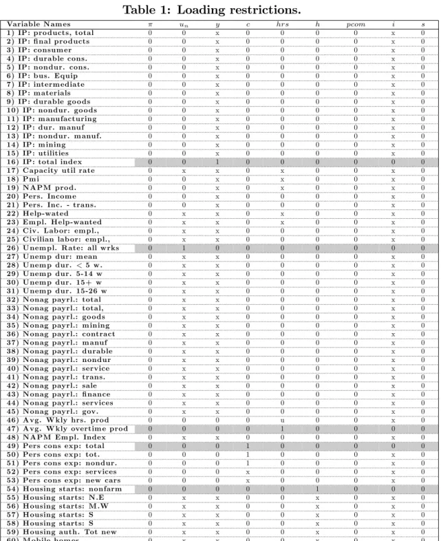
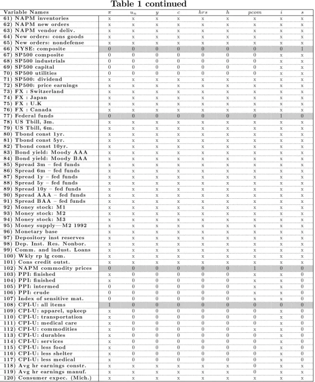
capturing information on nascent in‡ation pressures. Insert Table 1
Table 1 o¤ers an overview of the identi…cation restrictions. The identi…cation of the respective factors is obtained in two steps. First, we …x the interpretation of the factors by imposing a set of unbiasedness restrictions. In particular, we impose unbiasedness restrictions on nine observables closest to the economic in-terpretation of each of the factors (see shading areas in Table 1).12 This results in an exactly identi…ed system (along the lines of Proposition 2 in Geweke & Singleton (1981)). This exactly identi…ed latent factor model is labelled as the “unrestricted model ”.
Second, (over-) identifying restrictions are imposed in the form of exclusion re-strictions (see Table 1). Generally, the identi…cation scheme is based on two strategies. First, exclusion restrictions are primarily imposed on slow-moving variables while fast-moving observables are left unrestricted (except for housing starts and stock market observations).13 This modeling choice is motivated by
the idea that fast moving variables, containing a speculative component, can be considered as general and timely information variables for macroeconomic devel-opments. Second, we di¤erentiate between nominal, real, information, and policy factors. We de…ne: one nominal factor (in‡ation factor); four real factors (un-employment, economic activity, consumption, and hours in production factors); three information factors (housing, commodity price, and stock market factors);
12The target observables of the factors are: the CPI-all items index (series 108) for the
in‡ation factor ( ); the Unemployment Rate all workers (series 26) for the unemployment factor (un); the Industrial Production-total index (series 16) for the economic activity factor
(y); Personal Consumption Expenditure all items (series 49) for the consumption factor (c); Average weekly Hours of Production in manufacturing (series 47) for the hours in production factor (hrs); Housing Starts non-farm (series 54) for the housing factor (h); NAPM commodity price index (series 102) for the commodity price factor (pcom); The e¤ective federal funds rate (series 77) by the monetary policy rate factor (i); and …nally the NYSE stock price index (series 66) for the stock market factor (s). See appendix A for the de…nition and numbers assigned to each observable in the data panel.
13We use the de…nition of fast- and slow-moving variables of Bernanke et al. (2005) except
housing starts and stock market returns, which we assume not to respond contemporaneously to some factors. This assumption helps empirically to distinguish a housing factor from a stock market factor.
and one policy factor (monetary policy factor). In our identi…cation strategy, nominal factors exclude all types of real observables as (contemporaneous) in-formation variables. In the same way, real factors exclude nominal variables. Information factors exclude all slow-moving real and nominal observables. Fi-nally, the policy factor loads freely on all observables. Details on the restrictions per variable are listed in Table 1 and described in more detail in Appendix B. A …nal set of exclusion restrictions identi…es the structural shocks through a stan-dard Cholesky decomposition of the variance-covariance matrix of disturbances in the state equation. The ordering used in the analysis is as follows: ; un; y; c;
hrs; pcom; i; s: This ordering is in line with the identi…cation of monetary policy shocks in the literature (see for example Christiano et al. (1999)).
3.2
Empirical Results
3.2.1 Identi…cation restrictions and model performance
Our identi…cation scheme (see section 2) involves 482 over-identifying restrictions. In this section we provide a statistical test on these restrictions. In particular, we perform an LR-test of our restricted model against the unrestricted (exactly identi…ed) model. We complement this test by a number of measures of …t in-cluding R2, AIC, BIC; the log-likelihood value, and ICp2; a modi…ed version of
the Bai & Ng (2002) ICp2 panel information criterion (see Doz et al. (2006)).
Table 2 reports the results. As expected, the over-identifying restrictions are rejected at the usual signi…cance level. Moreover, the values of the information criteria (AIC, BIC and ICp2) are higher for the restricted model. Interestingly, despite the statistical rejection of the model, we observe that the economic costs of the restrictions is relatively small. In particular, the cost of imposing 482 over-identifying restrictions is a decrease in overall (simple average) R2 of
ap-proximately four percentage points, from 57:0% to 53:2%. As a result, little is lost by imposing the over-identifying restrictions and we are willing to pay the price of a slight reduction in overall R2 for economically interpretable factors.14
14Similar drops in R-square have been reported by Reis & Watson (2008). In a related
Insert Table 2
The general performance (explanatory power) of the restricted nine factor model is in line with the literature. Speci…cally, the average R2 of 53:2% of our model is
in line with the performance of large unrestricted DFMs for the US economy (e.g. Bai & Ng (2007), Bork (2008) and Yu (2008)). Also, the value of average R2 of
our model corresponds to the value one would obtain from the Stock & Watson (2002b) principal components approach with six factors. These …ndings suggest that the over-identifying restrictions and the implied economic interpretation of the factors can be obtained without major loss in …tting the dominant dimensions of variation in the panel.
3.2.2 Implied factors
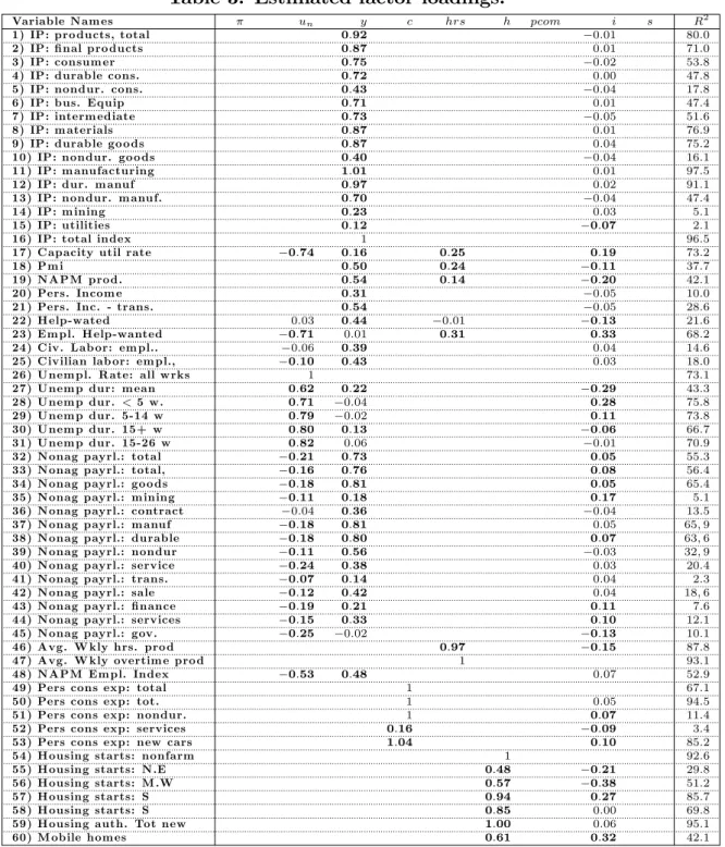
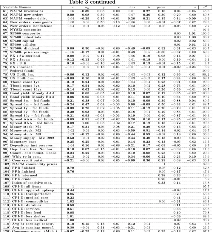
Table 3 reports the estimates of free factor loadings as well as the total variance explained by the common factors (R2) for each of our observables. Figures 1
till 3 give a graphical representation of the estimated factor loadings for each of the nine retained factors. Overall, the statistics reported in Table 3 support the economic interpretation of the latent factors. In particular, the signs of estimated factor loadings are in line with theory. Also, the retrieved factors capture most of the variation in the key variables (with many R2s above 90%). Figure 4 displays
the factors as retrieved from the panel.
Insert Figures 4 till 3 and Table 3
Speci…cally, we …nd that the in‡ation factor ( ) closely tracks the CPI-u all items in‡ation. Moreover, the R-squared is higher than the one based on the in‡ation factor identi…ed by Bernanke et al. (2005) (96% instead of 87%).15 The
estimated factor loadings on other CPI and PPI in‡ation series are signi…cantly positive and the common component captures a substantial part of the variation
each of 187 US sectoral price indices. Using t-tests they reject the null hypothesis of unit loadings on their pure in‡ation factor. They report that imposing these restrictions only decreases the R2 by less than 3% for eighty percent of the 187 observables.
in these series.
The unemployment factor (un) captures approximately 73% of the variation in
the target unemployment variable, i.e. Unemployment rate all workers. Other unemployment measures load signi…cantly and positively on this factor. Note too that this factor also contributes signi…cantly to the variation in the payroll variables and capacity utilization. As expected, loadings are typically negative for employment, payroll and capacity utilization variables.
The economic activity factor (y) explains up to 97% of growth in industrial pro-duction (the target variable) and also …ts reasonably well the di¤erent compo-nents of industrial production. Exceptions are non-durables, mining and utilities. Moreover, loadings for industrial production components are in general positive. The economic activity factor also contributes to the variation of payroll, income and employment variables. The consumption factor (c) is restricted to load only on the …ve personal expenditure series in addition to the fast-moving variables. The one-to-one restrictions help to extract a consumption factor that explains 67 percent in the total personal expenditure series which is signi…cantly higher than the 6-10% reported by Bernanke et al. (2005) and Bork (2008). Note too that estimated factor loadings suggest a close link between consumption of durables and the consumption factor. Other consumption components, i.e. non-durables and services, remain largely unrelated to the consumption factor as indicated by the low R2. The hours in production factor (hrs) explains average weekly
over-time hours for production workers in manufacturing almost perfectly, R2 = 93%.
Furthermore, as suggested by the loadings, this factor signi…cantly contributes to the dynamics of capacity utilization and help-wanted ads dynamics.
The housing factor (h) explains 93% of total non-farm housing starts and autho-rizations while the commodity price factor (pcom) only captures 39% in monthly commodity price in‡ation as measured by movement in the NAPM commodity price index. The stock market factor (s) explains more than 97% of variation in the NYSE index. This factor also explains well price movements for the S&P500. Price earnings or dividend ratios do not load signi…cantly on the stock market factor. The latter feature is probably explained by the fact that the stock mar-ket factor models stock returns, while levels of the price dividend and earnings
ratios are included in the data set. Finally, the monetary policy factor tracks, by construction, perfectly the federal funds rate. In addition, the factor explains most of the variation in the remaining interest rate variables such as yields and spreads. Loadings for yields and spreads conform to the standard term structure literature.
3.2.3 Measuring the impact of monetary policy
We use our model to analyze the overall impact of monetary policy shocks on the US economy. To facilitate comparison with the literature we do not present the impulse response functions (IRFs) of the factors themselves. Instead, we focus on the IRFs of twenty key measures covering the US economy, as implied by the fac-tor model (e.g. Bernanke et al. (2005)). More speci…cally, we analyze the federal funds rate, the yen per US dollar exchange rate, the level of industrial production, the consumer price level (CPI), monetary aggregates, the capacity utilization, the (un)employment level, the average hourly earnings, the level of consumption and consumer con…dence expectations as key indicators for the macroeconomy. Addi-tionally, we cover housing starts and two …nancial market indicators: the dividend yield on the S&P and the …ve year treasury yield.
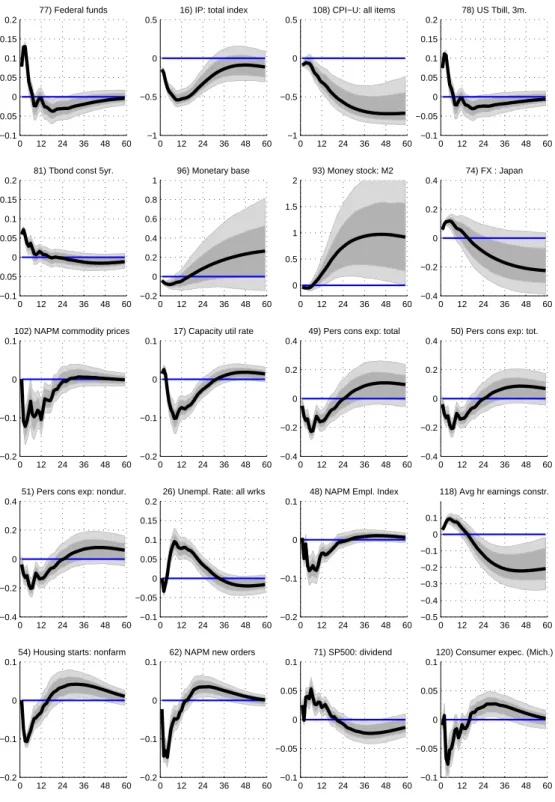
Insert Figure 5
Figure 5 displays the IRFs of each of these variables to a 25 basis points monetary policy shock. The unit of the IRFs is the standard deviation of the respective se-ries. Our IRFs depicted in Figure 5, are as expected and in line with the literature (see Christiano et al. (1999)). The empirical plausibility of the IRFs, therefore, suggests that the model is able to identify accurately the key macroeconomic transmission mechanisms and shocks.
Several observations can be made in this respect. First, unlike standard small-scale VAR models, we do no longer observe a price puzzle. Second, a contrac-tionary monetary policy shock has a negative impact on output where the maxi-mal e¤ect is reached within one year. Third, long-run neutrality of monetary
pol-icy cannot be rejected. In particular, monetary polpol-icy shocks only have a tempo-rary e¤ect on production, consumption, capacity utilization, and (un)employment levels. Fourth, the impact of temporary policy shocks is initially negative on the consumption expectations but then reverses before the impact becomes neutral in the long-run. Finally, the results show a signi…cant impact of monetary policy shocks on …nancial markets. Monetary policy tightening increases the bond yields with the short-term yields responding more than the long-term yields, as illus-trated by the IRF of the 3 month and 5 year yield. However, given the moderate persistence of the policy shocks (see the IRF of the federal funds rate), the impact on bond yields of monetary policy shocks remains relatively small and temporary. Real estate markets, as illustrated by the IRF of the housing starts, initially re-spond strongly to the monetary policy shock although there is no long-run e¤ect. Following a monetary tightening, the dividend yield tends to adjust temporarily upwards while the yen tends to depreciate against the US dollar. These IRFs match both the responses reported in Banbura et al. (2008), using a BVAR and Bernanke et al. (2005) using a FAVAR.
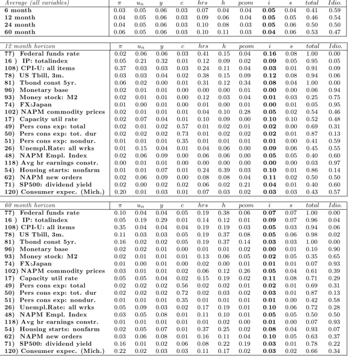
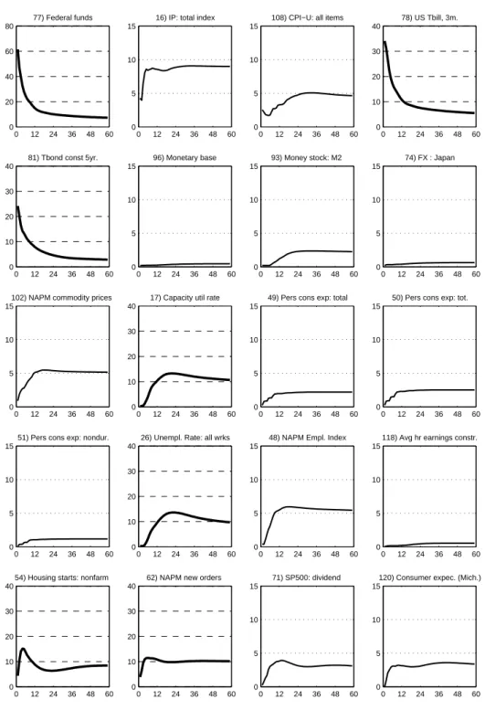
Insert Figure 6 and Table 4
Table 4 and Figure 6 present the variance decomposition of the selected vari-ables at alternative forecasting horizons. This tool allows us to assess the rel-ative importance of monetary policy shocks in the overall variation of the se-ries. Our results are broadly in line with those reported both in Banbura et al. (2008) and Bernanke et al. (2005). In line with these studies, we observe that monetary shocks do not have an important long-run (60 month) impact on the forecast error variance of a broad selection of key macroeconomic and …nancial variables. Speci…cally, we …nd that a monetary policy shock explains less than 12%of the variation in industrial production, consumer prices, commodity prices, (un)employment, new orders for any forecast horizon and virtually zero for con-sumption and money base. Unlike Bernanke et al. (2005), however, we do not …nd a large signi…cant long-run e¤ect of monetary policy shocks on the federal funds rate and the bond yields. The estimates reported in Table 4 indicate that monetary policy shocks are only mildly persistent and only account for
approx-imately 3% to 7% of total long-run variation in the federal funds rate and the bond yields. Banbura et al. (2008), reporting similarly small numbers, argue that this may be explained by the size of the model.16
4
Conclusion
This paper has proposed a methodology to identify factors within the framework of dynamic factor models. We impose an economic interpretation on the static factors through a set of over-identifying restrictions on the factor loadings. We modify the standard estimation methodology to incorporate these over-identifying loading restrictions. In particular, following Shumway & Sto¤er (1982) and Wu et al. (1996), the appropriate parameter estimators and …lters based on the EM algorithm are discussed.
In the empirical application the paper focuses on identifying a set of nine factors with economic interpretation. These factors represent key measures of the US economy such as in‡ation, unemployment, economic activity, consumption, state of the business cycle, residential investments, …nancial markets and monetary policy. The obtained factors are empirically plausible measures for each of the targeted key concepts, listed above. Subsequently, we use the model to assess the overall impact of monetary policy on the US economy. Our results are in line with those obtained using alternative methods on large panels, e.g. FAVARs or large BVARs.
16The larger the model, the more shocks can be identi…ed and the smaller the likelihood of
misspeci…cation of the monetary policy shocks. In this model we identify nine structural shocks, which is signi…cantly higher than the number of structural shocks identi…ed by Bernanke et al. (2005).
References
Alessi, L., Barigozzi, M. & Capasso, M. (2007), ‘Dynamic factor GARCH: Multi-variate volatility forecast for a large number of series’, Laboratory of Economics and Management (LEM), Sant’Anna School of Advanced Studies .
Altug, S. (1989), ‘Time to build and aggregate ‡uctuations: some new evidence’, International Economic Review 30(4), 889–920.
Bai, J. & Ng, S. (2002), ‘Determining the number of factors in approximate factor models’, Econometrica 70(1), 191–221.
Bai, J. & Ng, S. (2007), ‘Determining the number of primitive shocks in factor models’, Journal of Business & Economic Statistics 25, 52–60.
Banbura, M., Giannone, D. & Reichlin, L. (2008), ‘Large bayesian VARs’, Journal of Applied Econometrics (forthcoming) .
Bernanke, B. S. & Boivin, J. (2003), ‘Monetary policy in a data-rich environment’, Journal of Monetary Economics 50(3), 525–546.
Bernanke, B. S., Boivin, J. & Eliasz, P. (2005), ‘Measuring the e¤ects of mone-tary policy: a factor-augmented vector autoregressive (FAVAR) approach’, The Quarterly Journal of Economics pp. 387–422.
Bjørnland, H. & Leitemo, K. (2009), ‘Identifying the interdependence between US monetary policy and the stock market’, Journal of Monetary Economics (forthcoming) .
Blanchard, O. J. & Quah, D. (1989), ‘The dynamic e¤ects of aggregate demand and supply disturbances’, American Economic Review 79(4), 655–73.
Boivin, J. & Giannoni, M. (2006), Dsge models in a data-rich environment, Work-ing Paper 12772, National Bureau of Economic Research.
Boivin, J., Giannoni, M. P. & Mihov, I. (2009), ‘Sticky prices and monetary policy: Evidence from disaggregated us data’, American Economic Review 99(1), 350–84.
Bork, L. (2008), Estimating US monetary policy shocks using a factor-augmented vector autoregression: An EM algorithm approach. CREATES Research Paper 2009-11, University of Aarhus.
Campbell, J. Y., Lo, A. & MacKinlay, C. (1997, ch. 2), The Econometrics of Financial Markets, Princeton University Press, Princeton.
Chamberlain, G. & Rothschild, M. (1983), ‘Arbitrage, factor structure, and mean-variance analysis on large asset markets’, Econometrica 51(5), 1281–1304. Christiano, L. J., Eichenbaum, M. & Evans, C. L. (1999), Monetary policy shocks:
What have we learned and to what end?, in J. B. Taylor & M. Woodford, eds, ‘Handbook of Macroeconomics’, Vol. 1A, Elsevier Science, North Holland, New York, pp. 65–148.
de Jong, P. (1989), ‘Smoothing and interpolation with the state-space model’, Journal of the American Statistical Association 84, 1085–1088.
de Jong, P. & Mackinnon, M. J. (1988), ‘Covariances for smoothed estimates in state space models’, Biometrika (75), 601–602.
Diebold, F. X., Li, C. & Yue, V. Z. (2008), ‘Global yield curve dynamics and interactions: A dynamic Nelson-Siegel approach’, Journal of Econometrics 146(2), 351–363.
Doz, C., Giannone, D. & Reichlin, L. (2006), A quasi maximum likelihood ap-proach for large approximate dynamic factor models. European Central Bank Working Paper no. 674.
Doz, C., Giannone, D. & Reichlin, L. (2007), A two-step estimator for large ap-proximate dynamic factor models based on Kalman …ltering, CEPR Discussion Paper 6043, Centre for Economic Policy Research.
Forni, M., Giannone, D., Lippi, M. & Reichlin, L. (2008), ‘Opening the black box: Structural factor models with large cross-sections’, Econometric Theory, Vol. 25, No. 05, Pages 1319-1347 .
Forni, M., Hallin, M., Lippi, M. & Reichlin, L. (2000), ‘The generalized dynamic-factor model: Identi…cation and estimation’, The Review of Economics and Statistics 82(4), 540–554.
Forni, M., Hallin, M., Lippi, M. & Reichlin, L. (2001), ‘Coincident and leading indicators for the euro area’, Economic Journal 111(471), 62–85.
Forni, M., Hallin, M., Lippi, M. & Reichlin, L. (2005), ‘The generalized dynamic factor model: one sided estimation and forecasting’, Journal of the American Statistical Association 100(471), 830–840.
Forni, M. & Lippi, M. (2001), ‘The generalized dynamic factor model: Represen-tation theory’, Econometric Theory 17(06), 1113–1141.
Forni, M. & Reichlin, L. (1998), ‘Let’s get real: A factor analytical ap-proach to disaggregated business cycle dynamics’, Review of Economic Studies 65(3), 453–73.
Forni, M. & Reichlin, L. (2001), ‘Federal policies and local economies: Europe and the us’, European Economic Review 45(1), 109–134.
Geweke, J. F. & Singleton, K. J. (1981), ‘Maximum likelihood "con…rmatory" fac-tor analysis of economic time series’, International Economic Review 22(1), 37– 54.
Giannone, D., Reichlin, L. & Sala, L. (2002), Tracking Greenspan: Systematic and unsystematic monetary policy revisited. CEPR Discussion Papers no. 3550. Giannone, D., Reichlin, L. & Sala, L. (2004), Monetary policy in real time, in M. Gertler & K. Rogo¤, eds, ‘NBER Macroeconomic Annual 2004’, Vol. 19, MIT Press.
Hallin, M. & Liska, R. (2007), ‘Determining the number of factors in the general-ized factor model’, Journal of the American Statistical Association 102, 603– 617.
Houssa, R. (2008a), ‘Monetary union in west africa and asymmetric shocks: A dynamic structural factor model approach’, Journal of Development Economics Vol. 85, 319–347.
Houssa, R. (2008b), Sources of Fluctuations: World, Regional, and National Factors, In Macroeconomic Fluctuations in Developing Countries, PhD the-sis, KULeuven.
Ingersoll, Jonathan E, J. (1984), ‘Some results in the theory of arbitrage pricing’, Journal of Finance 39(4), 1021–39.
Jungbacker, B. & Koopman, S. J. (2008), Likelihood-based analysis for dynamic factor models, Tinbergen Institute Discussion Papers 08-007/4, Tinbergen In-stitute.
Kim, C.-J. & Nelson, C. R. (1999), State-Space Models with Regime Switching, The MIT Press.
Kose, A. M., Otrok, C. & Whiteman, C. (2003), ‘International business cy-cles: World, region, and country-speci…c factors’, American Economic Review 93(4), 1216–1239.
Lawley, D. N. & Maxwell, A. E. (1971), Factor Analysis as a Statistical Method (Butterworths Mathematical Texts), 2nd. edn, Butterworths, London.
Leeper, E. M., Sims, C. A. & Zha, T. (1996), ‘What does monetary policy do?’, Brookings Papers on Economic Activity 27(1996-2), 1–78.
Ludvigson, S. C. & Ng, S. (2007), ‘The empirical risk-return relation: A factor analysis approach’, Journal of Financial Economics 83(1), 171–222.
Ludvigson, S. C. & Ng, S. (2008), ‘Macro factors in bond risk premia’, The Review of Financial Studies (forthcoming) .
Mönch, E. (2008), ‘Forecasting the yield curve in a data-rich environment: A no-arbitrage factor-augmented VAR approach’, Journal of Econometrics 146(1), 26–43.
Otrok, C. & Whiteman, C. H. (1998), ‘Bayesian leading indicators: Measuring and predicting economic conditions in Iowa’, International Economic Review 39(4), 997–1014.
Reis, R. & Watson, M. W. (2008), Relative goods’prices, pure in‡ation, and the Philips correlation. American Economic Journal Macroeconomics (forthcom-ing).
Sargent, T. J. (1989), ‘Two models of measurements and the investment acceler-ator’, Journal of Political Economy 97(2), 251–287.
Shumway, R. H. & Sto¤er, D. S. (1982), ‘An approach to time series smoothing and forecasting using the EM algorithm’, Journal of Time Series Analysis 3, 253–226.
Sims, C. (1980), ‘Macroeconomics and reality’, Econometrica 48, 1–48.
Stock, J. H. & Watson, M. W. (2002a), ‘Forecasting using principal components from a large number of predictors’, Journal of the American Statistical Asso-ciation 97, 1167–1179.
Stock, J. H. & Watson, M. W. (2002b), ‘Macroeconomic forecasting using di¤usion indexes’, Journal of Business Economics and Statistics XX:II, 147–162. Stock, J. H. & Watson, M. W. (2005), Implications of dynamic factor models for
VAR analysis, Working Paper 11467, National Bureau of Economic Research. Uhlig, H. (2005), ‘What are the e¤ects of monetary policy on output? Results
from an agnostic identi…cation procedure’, Journal of Monetary Economics 52(2), 381–419.
Wu, L. S.-Y., Pai, J. S. & Hosking, J. (1996), ‘An algorithm for estimating parameters of state-space models’, Statistics and Probability Letters 28, 99– 106.
Yu, W.-C. (2008), ‘Macroeconomic and …nancial market volatilities: an empirical evidence of factor model’, Economics Bulletin 3(33), 1–18.
A
Data description
Data are from Bernanke et al. (2005).
First column: A superscript indicates that an exactly identifying restriction has been imposed on this variable, i.e. 108[1] indicates that an identifying restriction has been imposed on this variable for the …rst factor. The second column is a mnemonic and a * indicates a "slow-moving" variable. Fourth column contains transformation codes. "level" indicates an un-transformed variable, say xt: "ln" means ln xtand " ln" means
ln xt ln xt 1:
Real output and income
1 IPP* 1959:01–2001:08 ln Industrial production: products, total (1992 = 100,SA) 2 IPF* 1959:01–2001:08 ln Industrial production: …nal products (1992 = 100,SA) 3 IPC* 1959:01–2001:08 ln Industrial production: consumer goods (1992 = 100,SA) 4 IPCD* 1959:01–2001:08 ln Industrial production: durable cons. goods (1992 = 100,SA) 5 IPCN* 1959:01–2001:08 ln Industrial production: nondurable cons. goods (1992 = 100,SA) 6 IPE* 1959:01–2001:08 ln Industrial production: business equipment (1992 = 100,SA) 7 IPI* 1959:01–2001:08 ln Industrial production: intermediate products (1992 = 100,SA) 8 IPM* 1959:01–2001:08 ln Industrial production: materials (1992 = 100,SA)
9 IPMD* 1959:01–2001:08 ln Industrial production: durable goods materials (1992 = 100,SA) 10 IPMND* 1959:01–2001:08 ln Industrial production: nondur. goods materials (1992 = 100,SA) 11 IPMFG* 1959:01–2001:08 ln Industrial production: manufacturing (1992 = 100,SA)
12 IPD* 1959:01–2001:08 ln Industrial production: durable manufacturing (1992 = 100,SA) 13 IPN* 1959:01–2001:08 ln Industrial production: nondur. manufacturing (1992 = 100,SA) 14 IPMIN* 1959:01–2001:08 ln Industrial production: mining (1992 = 100,SA)
15 IPUT* 1959:01–2001:08 ln Industrial production: utilities (1992 = 100,SA) 16[3] IP* 1959:01–2001:08 ln Industrial production: total index (1992 = 100,SA)
17 IPXMCA* 1959:01–2001:08 level Capacity util rate: manufac., total (% of capacity,SA) (frb) 18 PMI* 1959:01–2001:08 level Purchasing managers’ index (SA)
19 PMP* 1959:01–2001:08 level NAPM production index (percent)
20 GMPYQ* 1959:01–2001:08 ln Personal income (chained) (series #52) (bil 92$,SAAR)
(Un)employment and hours
22 LHEL* 1959:01–2001:08 ln Index of help-wanted advertising in newspapers (1967 = 100;SA) 23 LHELX* 1959:01–2001:08 ln Employment: ratio; help-wanted ads: no. unemployed clf 24 LHEM* 1959:01–2001:08 ln Civilian labor force: employed, total (thous.,SA)
25 LHNAG* 1959:01–2001:08 ln Civilian labor force: employed, nonag. industries (thous.,SA) 26[2] LHUR* 1959:01–2001:08 level Unemployment rate: all workers, 16 years and over (%,SA)
27 LHU680* 1959:01–2001:08 level Unemploy. by duration: average (mean) duration in weeks (SA) 28 LHU5* 1959:01–2001:08 level Unemploy. by duration: pers unempl. less than 5 wks (thous.,SA) 29 LHU14* 1959:01–2001:08 level Unemploy. by duration: pers unempl. 5 to 14 wks (thous.,SA) 30 LHU15* 1959:01–2001:08 level Unemploy. by duration: pers unempl. 15 wks = (thous.,SA) 31 LHU26* 1959:01–2001:08 level Unemploy. by duration: pers unempl. 15 to 26 wks (thous.,SA) 32 LPNAG* 1959:01–2001:08 ln Employees on nonag. payrolls: total (thous.,SA)
33 LP* 1959:01–2001:08 ln Employees on nonag. payrolls: total, private (thous.,SA) 34 LPGD* 1959:01–2001:08 ln Employees on nonag. payrolls: goods-producing (thous.,SA) 35 LPMI* 1959:01–2001:08 ln Employees on nonag. payrolls: mining (thous.,SA)
36 LPCC* 1959:01–2001:08 ln Employees on nonag. payrolls: contract construc. (thous.,SA) 37 LPEM* 1959:01–2001:08 ln Employees on nonag. payrolls: manufacturing (thous.,SA) 38 LPED* 1959:01–2001:08 ln Employees on nonag. payrolls: durable goods (thous.,SA) 39 LPEN* 1959:01–2001:08 ln Employees on nonag. payrolls: nondurable goods (thous.,SA) 40 LPSP* 1959:01–2001:08 ln Employees on nonag. payrolls: service-producing (thous.,SA) 41 LPTU* 1959:01–2001:08 ln Employees on nonag. payrolls: trans. and public util. (thous.,SA) 42 LPT* 1959:01–2001:08 ln Employees on nonag. payrolls: wholesale and retail (thous.,SA) 43 LPFR* 1959:01–2001:08 ln Employees on nonag. payrolls: …nance, ins. and real est (thous.,SA) 44 LPS* 1959:01–2001:08 ln Employees on nonag. payrolls: services (thous.,SA)
45 LPGOV* 1959:01–2001:08 ln Employees on nonag. payrolls: government (thous.,SA) 46 LPHRM* 1959:01–2001:08 level Avg. weekly hrs. of production wkrs.: manufacturing (sa) 47[5] LPMOSA* 1959:01–2001:08 level Avg. weekly hrs. of prod. wkrs.: mfg., overtime hrs. (sa)
48 PMEMP* 1959:01–2001:08 level NAPM employment index (percent)
Consumption
49[4] GMCQ* 1959:01–2001:08 ln Pers cons exp (chained)— total (bil 92$,SAAR)
50 GMCDQ* 1959:01–2001:08 ln Pers cons exp (chained)— tot. dur. (bil 96$,SAAR) 51 GMCNQ* 1959:01–2001:08 ln Pers cons exp (chained)— nondur. (bil 92$,SAAR) 52 GMCSQ* 1959:01–2001:08 ln Pers cons exp (chained)— services (bil 92$,SAAR) 53 GMCANQ* 1959:01–2001:08 ln Personal cons expend (chained)— new cars (bil 96$,SAAR)
Housing starts and sales
54[6] HSFR 1959:01–2001:08 ln Housing starts: nonfarm (1947–1958); tot. (
55 HSNE 1959:01–2001:08 ln Housing starts: northeast (thous.u.)s.a. 56 HSMW 1959:01–2001:08 ln Housing starts: midwest (thous.u.)s.a. 57 HSSOU 1959:01–2001:08 ln Housing starts: south (thous.u.)s.a. 58 HSWST 1959:01–2001:08 ln Housing starts: west (thous.u.)s.a.
59 HSBR 1959:01–2001:08 ln Housing authorized: total new priv housing (thous.,SAAR) 60 HMOB 1959:01–2001:08 ln Mobile homes: manufacturers’ shipments (thous. of units,SAAR)
Real inventories, ordes and un…lled orders
61 MNV 1959:01–2001:08 level NAPM inventories index (percent) 62 PMNO 1959:01–2001:08 level NAPM new orders index (percent) 63 PMDEL 1959:01–2001:08 level NAPM vendor deliveries index (percent)
64 MOCMQ 1959:01–2001:08 ln New orders (net)— consumer goods and materials, 1992 $ (bci) 65 MSONDQ 1959:01–2001:08 ln New orders, nondefense capital goods, in 1992 $s (bci)
Stock prices
66[9] FSNCOM 1959:01–2001:08 ln NYSE composite (12/31/65 = 50)
67 FSPCOM 1959:01–2001:08 ln S&P’s composite (1941–1943 = 10) 68 FSPIN 1959:01–2001:08 ln S&P’s industrials (1941–1943 = 10) 69 FSPCAP 1959:01–2001:08 ln S&P’s capital goods (1941–1943 = 10) 70 FSPUT 1959:01–2001:08 ln S&P’s utilities (1941–1943 = 10)
71 FSDXP 1959:01–2001:08 level S&P’s composite common stock: dividend yield (% per annum) 72 FSPXE 1959:01–2001:08 level S&P’s composite common stock: price-earnings ratio (%,NSA)
Foreign exchange rates
73 EXRSW 1959:01–2001:08 ln Foreign exchange rate: Switzerland (swiss franc per US$) 74 EXRJAN 1959:01–2001:08 ln Foreign exchange rate: Japan (yen per US$)
75 EXRUK 1959:01–2001:08 ln Foreign exchange rate: United Kingdom (cents per pound) 76 EXRCAN 1959:01–2001:08 ln Foreign exchange rate: Canada (canadian $ per US$)
Interest rates and spreads
77[8] FYFF 1959:01–2001:08 level Interest rate: federal funds (e¤ective) (% per annum,nsa) 78 FYGM3 1959:01–2001:08 level Interest rate: us tbill,sec mkt,3-mo. (% per ann,nsa) 79 FYGM6 1959:01–2001:08 level Interest rate: us tbill,sec mkt,6-mo. (% per ann,nsa) 80 FYGT1 1959:01–2001:08 level Interest rate: ust const matur., 1-yr. (% per ann,nsa) 81 FYGT5 1959:01–2001:08 level Interest rate: ust const matur., 5-yr. (% per ann,nsa) 82 FYGT10 1959:01–2001:08 level Interest rate: ust const matur., 10-yr. (% per ann,nsa) 83 FYAAAC 1959:01–2001:08 level Bond yield: moody’s aaa corporate (% per annum) 84 FYBAAC 1959:01–2001:08 level Bond yield: moody’s baa corporate (% per annum) 85 SFYGM3 1959:01–2001:08 level Spread fygM3— fy¤
86 SFYGM6 1959:01–2001:08 level Spread fygm6— fy¤ 87 SFYGT1 1959:01–2001:08 level Spread fygt1— fy¤ 88 SFYGT5 1959:01–2001:08 level Spread fygt5— fy¤ 89 SFYGT10 1959:01–2001:08 level Spread fygt10— fy¤ 90 SFYAAAC 1959:01–2001:08 level Spread fyaaac— fy¤ 91 SFYBAAC 1959:01–2001:08 level Spread fybaac— fy¤
Money and credit quantity aggregates
92 FM1 1959:01–2001:08 ln Money stock: M1 (bil$,SA) 93 FM2 1959:01–2001:08 ln Money stock: M2 (bil$,SA) 94 FM3 1959:01–2001:08 ln Money stock: M3 (bil$,SA) 95 FM2DQ 1959:01–2001:08 ln Money supply— M2 in 1992 $s (bci)
96 FMFBA 1959:01–2001:08 ln Monetary base, adj for reserve requirement changes (mil$,SA) 97 FMRRA 1959:01–2001:08 ln Depository inst reserves: total, adj for res. req chgs (mil$,SA) 98 FMRNBA 1959:01–2001:08 ln Depository inst reserves: nonbor., adj res req chgs (mil$,SA) 99 FCLNQ 1959:01–2001:08 ln Commercial and indust. loans outstanding in 1992 $s (bci)
100 FCLBMC 1959:01–2001:08 level Wkly rp lg com. banks: net change com and ind. loans (bil$,SAAR) 101 CCINRV 1959:01–2001:08 ln Consumer credit outstanding nonrevolving g19
Price indexes
102[7] PMCP 1959:01–2001:08 level NAPM commodity prices index (%)
103 PWFSA* 1959:01–2001:08 ln PPI: …nished goods (82 = 100,SA)
104 PWFCSA* 1959:01–2001:08 ln PPI: …nished consumer goods (82 = 100,SA)
105 PWIMSA* 1959:01–2001:08 ln PPI: intermed mat. sup and components (82 = 100,SA) 106 PWCMSA* 1959:01–2001:08 ln PPI: crude materials (82 = 100,SA)
107 PSM99Q* 1959:01–2001:08 ln Index of sensitive materials prices (1990 = 100) (bci-99a) 108[1] PUNEW* 1959:01–2001:08 ln CPI-u: all items (82–84 = 100,SA)
109 PU83* 1959:01–2001:08 ln CPI-u: apparel and upkeep (82–84 = 100,SA) 110 PU84* 1959:01–2001:08 ln CPI-u: transportation (82–84 = 100,SA) 111 PU85* 1959:01–2001:08 ln CPI-u: medical care (82–84 = 100,SA) 112 PUC* 1959:01–2001:08 ln CPI-u: commodities (82–84 = 100,SA) 113 PUCD* 1959:01–2001:08 ln CPI-u: durables (82–84 = 100,SA) 114 PUS* 1959:01–2001:08 ln CPI-u: services (82–84 = 100,SA)
115 PUXF* 1959:01–2001:08 ln CPI-u: all items less food (82–84 = 100,SA) 116 PUXHS* 1959:01–2001:08 ln CPI-u: all items less shelter (82–84 = 100,SA) 117 PUXM* 1959:01–2001:08 ln CPI-u: all items less medical care (82– 84 = 100,SA)
Average hourly earnings
118 LEHCC* 1959:01–2001:08 ln Avg hr earnings of constr wkrs: construction ($,SA) 119 LEHM* 1959:01–2001:08 ln Avg hr earnings of prod wkrs: manufacturing ($,SA)
Miscellaneous
B
Over-identifying loading restrictions
The speci…c set of (over-) identifying restrictions can be summarized as follows; the in‡ation factor ( ) is identi…ed by the unbiasedness restriction on CPI-u all items. Additionally, we allow other in‡ation measures to load on the in‡ation factor. With the in‡ation factor being a nominal factor, we exclude from the information set all real variables, e.g. industrial production.
For the four real factors we impose exclusion restrictions on nominal variables (e.g. CPI in‡ation). Additional exclusion restrictions limit the type of real vari-ables acting as information varivari-ables for each of the factors. In particular, the unemployment factor (un)is identi…ed by the unbiasedness restriction on
’Unem-ployment all workers’. Other (un)em’Unem-ployment variables and measures of payroll statistics and capacity utilization are included as additional information vari-ables. All other slow-moving variables are excluded from the information set. The economic activity factor (y), identi…ed by the unbiasedness restriction on the Industrial Production (IP) total index series, uses IP variables next to em-ployment and payroll series as additional state variables. The hours in production factor (hrs) measures the current over (under) production and is identi…ed (by means of an unbiasedness restriction) through the overtime hours in production and manufacturing. As additional information variables we include variables such as capacity utilization rate, survey-based production indices (PMI, PMP) and help-wanted advertising to enter freely. We exclude (un)employment and IP growth as we consider them less informative with respect to the level of over and underproduction. The last real factor, i.e. the consumption factor (c) ; is …ltered from the observed consumption series in the panel with an unbiasedness restric-tion on ‘Personal Consumprestric-tion Expenditure’ series and one-to-one restricrestric-tions on two consumption observables. Moreover, due to consumption smoothing, we do not expect strong contemporaneous correlations between production employ-ment based statistics and consumption (growth). Therefore, we impose exclusion restrictions on production related variables.
The information and the policy factors measure particular features in the econ-omy. More precisely, the housing factor (h) is included as a residential investment
factor. This factor is identi…ed through an unbiasedness restriction on the total number of housing starts and uses as additional information variables other hous-ing starts or authorization variables. We consider the houshous-ing factor to be mainly a forward-looking variable containing all relevant information. As such, exclusion restrictions are imposed on all slow-moving variables. The commodity price fac-tor (pcom) aims at measuring cost-push facfac-tors due to price increases of raw materials or intermediate products. It is identi…ed by means of the NAPM com-modity price index. Moreover, the comcom-modity price factor retrieves additional information from PPI data for crude and intermediate materials and from the index of sensitive materials. The monetary policy factor (i) is directly measured by the e¤ective federal funds rate. Finally, the stock market factor (s) is related to returns on the NYSE index and uses S&P500 stock market component indices as additional state variables. We allow all other fast-moving variables to load freely on the stock market factor allowing for direct interactions across …nancial markets.
Table 1: Loading restrictions.
Variable N am es un y c hrs h pcom i s
1) IP : pro ducts, total 0 0 x 0 0 0 0 x 0 2) IP : …nal pro ducts 0 0 x 0 0 0 0 x 0 3) IP : consum er 0 0 x 0 0 0 0 x 0 4) IP : durable cons. 0 0 x 0 0 0 0 x 0 5) IP : nondur. cons. 0 0 x 0 0 0 0 x 0 6) IP : bus. Equip 0 0 x 0 0 0 0 x 0 7) IP : interm ediate 0 0 x 0 0 0 0 x 0 8) IP : m aterials 0 0 x 0 0 0 0 x 0 9) IP : durable go o ds 0 0 x 0 0 0 0 x 0 10) IP : nondur. go o ds 0 0 x 0 0 0 0 x 0 11) IP : m anufacturing 0 0 x 0 0 0 0 x 0 12) IP : dur. m anuf 0 0 x 0 0 0 0 x 0 13) IP : nondur. m anuf. 0 0 x 0 0 0 0 x 0 14) IP : m ining 0 0 x 0 0 0 0 x 0 15) IP : utilities 0 0 x 0 0 0 0 x 0 16) IP : total index 0 0 1 0 0 0 0 0 0 17) C apacity util rate 0 x x 0 x 0 0 x 0
18) P m i 0 0 x 0 x 0 0 x 0
19) N A P M pro d. 0 0 x 0 x 0 0 x 0 20) Pers. Incom e 0 0 x 0 0 0 0 x 0 21) Pers. Inc. - trans. 0 0 x 0 0 0 0 x 0 22) H elp-wated 0 x x 0 x 0 0 x 0 23) Em pl. H elp-wanted 0 x x 0 x 0 0 x 0 24) C iv. Lab or: em pl., 0 x x 0 0 0 0 x 0 25) C ivilian lab or: em pl., 0 x x 0 0 0 0 x 0 26) U nem pl. R ate: all w rks 0 1 0 0 0 0 0 0 0 27) U nem p dur: m ean 0 x x 0 0 0 0 x 0 28) U nem p dur. < 5 w . 0 x x 0 0 0 0 x 0 29) U nem p dur. 5-14 w 0 x x 0 0 0 0 x 0 30) U nem p dur. 15+ w 0 x x 0 0 0 0 x 0 31) U nem p dur. 15-26 w 0 x x 0 0 0 0 x 0 32) N onag payrl.: total 0 x x 0 0 0 0 x 0 33) N onag payrl.: total, 0 x x 0 0 0 0 x 0 34) N onag payrl.: go o ds 0 x x 0 0 0 0 x 0 35) N onag payrl.: m ining 0 x x 0 0 0 0 x 0 36) N onag payrl.: contract 0 x x 0 0 0 0 x 0 37) N onag payrl.: m anuf 0 x x 0 0 0 0 x 0 38) N onag payrl.: durable 0 x x 0 0 0 0 x 0 39) N onag payrl.: nondur 0 x x 0 0 0 0 x 0 40) N onag payrl.: service 0 x x 0 0 0 0 x 0 41) N onag payrl.: trans. 0 x x 0 0 0 0 x 0 42) N onag payrl.: sale 0 x x 0 0 0 0 x 0 43) N onag payrl.: …nance 0 x x 0 0 0 0 x 0 44) N onag payrl.: services 0 x x 0 0 0 0 x 0 45) N onag payrl.: gov. 0 x x 0 0 0 0 x 0 46) A vg. W kly hrs. pro d 0 0 0 0 u 0 0 x 0 47) A vg. W kly overtim e pro d 0 0 0 0 1 0 0 0 0 48) N A P M Em pl. Index 0 x x 0 0 0 0 x 0 49) Pers cons exp: total 0 0 0 1 0 0 0 0 0 50) Pers cons exp: tot. 0 0 0 1 0 0 0 x 0 51) Pers cons exp: nondur. 0 0 0 1 0 0 0 x 0 52) Pers cons exp: services 0 0 0 x 0 0 0 x 0 53) Pers cons exp: new cars 0 0 0 x 0 0 0 x 0 54) H ousing starts: nonfarm 0 0 0 0 0 1 0 0 0 55) H ousing starts: N .E 0 x x 0 0 x 0 x 0 56) H ousing starts: M .W 0 x x 0 0 x 0 x 0 57) H ousing starts: S 0 x x 0 0 x 0 x 0 58) H ousing starts: S 0 x x 0 0 x 0 x 0 59) H ousing auth. Tot new 0 x x 0 0 x 0 x 0 60) M obile hom es 0 x x 0 0 x 0 x 0
The factors are denoted by the symbols f ; un; y; c; hrs; h; pcom; i; sg and describe general in‡ation, unemployment,
economic activity (growth), consumption growth, hours in production, residential investments, commodity price in‡ation, federal funds rate and stock markets returns respectively. x denotes a free factor loading that is estimated. Shading areas cover loadings that are …xed with unbiasedness restrictions.
Table 1 continued Variable N am es un y c hrs h pcom i s 61) N A P M inventories x x x x x x x x x 62) N A P M new orders x x x x x x x x x 63) N A P M vendor deliv. x x x x x x x x x 64) N ew orders: cons go o ds x x x x x x x x x 65) N ew orders: nondefense x x x x x x x x x 66) N Y SE: com p osite 0 0 0 0 0 0 0 0 1 67) SP 500 com p osite 0 0 0 0 0 0 0 x x 68) SP 500 industrials 0 0 0 0 0 0 0 x x 69) SP 500 capital 0 0 0 0 0 0 0 x x 70) SP 500 utilities 0 0 0 0 0 0 0 x x 71) SP 500: dividend x x x x x x x x x 72) SP 500: price earnings x x x x x x x x x 73) FX : Sw itzerland x x x x x x x x x 74) FX : Japan x x x x x x x x x 75) FX : U .K x x x x x x x x x 76) FX : C anada x x x x x x x x x 77) Federal funds 0 0 0 0 0 0 0 1 0 78) U S T bill, 3m . x x x x x x x x x 79) U S T bill, 6m . x x x x x x x x x 80) T b ond const 1yr. x x x x x x x x x 81) T b ond const 5yr. x x x x x x x x x 82) T b ond const 10yr. x x x x x x x x x 83) B ond yield: M o o dy A A A x x x x x x x x x 84) B ond yield: M o o dy B A A x x x x x x x x x 85) Spread 3m – fed funds x x x x x x x x x 86) Spread 6m – fed funds x x x x x x x x x 87) Spread 1y – fed funds x x x x x x x x x 88) Spread 5y – fed funds x x x x x x x x x 89) Spread 10y – fed funds x x x x x x x x x 90) Spread A A A – fed funds x x x x x x x x x 91) Spread B A A – fed funds x x x x x x x x x 92) M oney sto ck: M 1 x x x x x x x x x 93) M oney sto ck: M 2 x x x x x x x x x 94) M oney sto ck: M 3 x x x x x x x x x 95) M oney supply— M 2 1992 x x x x x x x x x 96) M onetary base x x x x x x x x x 97) D ep ository inst reserves x x x x x x x x x 98) D ep. Inst. R es. N onb or. x x x x x x x x x 99) C om m . and indust. Loans x x x x x x x x x 100) W kly rp lg com . x x x x x x x x x 101) C ons credit outst. x x x x x x x x x 102) N A P M com m o dity prices 0 0 0 0 0 0 1 0 0 103) P P I: …nished x 0 0 0 0 0 x x 0 104) P P I: …nished x 0 0 0 0 0 x x 0 105) P P I: interm ed 0 0 0 0 0 0 x x 0 106) P P I: crude 0 0 0 0 0 0 x x 0 107) Index of sensitive m at. 0 0 0 0 0 0 x x 0 108) C P I-U : all item s 1 0 0 0 0 0 0 0 0 109) C P I-U : apparel, upkeep x 0 0 0 0 0 0 x 0 110) C P I-U : transp ortation x 0 0 0 0 0 0 x 0 111) C P I-U : m edical care x 0 0 0 0 0 0 x 0 112) C P I-U : com m o dities x 0 0 0 0 0 x x 0 113) C P I-U : durables x 0 0 0 0 0 0 x 0 114) C P I-U : services x 0 0 0 0 0 0 x 0 115) C P I-U : less fo o d x 0 0 0 0 0 0 x 0 116) C P I-U : less shelter x 0 0 0 0 0 0 x 0 117) C P I-U : less m edical x 0 0 0 0 0 0 x 0 118) A vg hr earnings constr. x x x x x x 0 x x 119) A vg hr earnings m anuf. x x x x x x 0 x x 120) C onsum er exp ec. (M ich.) x x x x x x x x x
The factors are denoted by the symbols f ; un; y; c; hrs; h; pcom; i; sg and describe general in‡ation, unemployment,
economic activity (growth), consumption growth, hours in production, residential investments, commodity price in‡ation, federal funds rate and stock markets returns respectively. x denotes a free factor loading that is estimated. Shading areas cover loadings that are …xed with unbiasedness restrictions.
Table 2: Model Performance.
R2 AIC BIC IC
p2 Log Lik p-value for LR test
Exactly Identi…ed Model 57:0 1:449 1:684 0:565 42821
Our (Restricted) Model 53:2 1:518 1:685 0:475 45413 0:0002
R2is a simple average of the R-squared of the 120 series; AIC denotes Akaike Information Criterion; BIC is Bayesian
Information Criterion; ICp2is a modi…ed version of the Bai & Ng (2002) ICp2information criterion; and Log Lik is