HAL Id: hal-00103149
https://hal.archives-ouvertes.fr/hal-00103149
Submitted on 3 Oct 2006
HAL is a multi-disciplinary open access
archive for the deposit and dissemination of sci-entific research documents, whether they are pub-lished or not. The documents may come from teaching and research institutions in France or abroad, or from public or private research centers.
L’archive ouverte pluridisciplinaire HAL, est destinée au dépôt et à la diffusion de documents scientifiques de niveau recherche, publiés ou non, émanant des établissements d’enseignement et de recherche français ou étrangers, des laboratoires publics ou privés.
Mixing enhancement and transport reduction in chaotic
advection
Tounsia Benzekri, Cristel Chandre, Xavier Leoncini, Ricardo Lima, Michel
Vittot
To cite this version:
Tounsia Benzekri, Cristel Chandre, Xavier Leoncini, Ricardo Lima, Michel Vittot. Mixing enhance-ment and transport reduction in chaotic advection. 5e Colloque Chaos Temporel et chaos Spatio-Temporel, Dec 2005, havre, France. pp.95-99. �hal-00103149�
ccsd-00103149, version 1 - 3 Oct 2006
chaotic advection
T.Benzekri
1, C.Chandre
1, X.Leoncini
1, R.Lima
1, & M.Vittot
1Centre de Physique Th´eorique⋆⋆, CNRS Luminy, Case 907, F-13288 Marseille cedex 9, France
benzekri@cpt.univ-mrs.fr
Abstract. We present a method for reducing chaotic transport in a model of chaotic advection due to time-periodic forcing of an oscillating vortex chain. We show that by a suitable modification of this forcing, the modified model combines two effects: enhancement of mixing within the rolls and suppression of chaotic transport along the channel.
1
Introduction
Chaotic advection (or Lagrangian chaos) was introduced in Ref. [1] to qualify a motion in which it is possible to generate chaotic trajectories even if the flow is laminar. Such phenomena are observed in a wide range of physical systems [2] and has fundamental applications such as in geophysical flow [3,4] and chemical engineering. Chaotic advection was mostly studied for two dimensional unsteady flows [5,6,8]. The advantage of these studies is that it uses the theory of dynamical systems and in particular the Hamiltonian theory for incompressible flows; the phase space being the physical space in this case. We present a method of chaos control for Hamiltonian systems, which is able by a small modification of the Hamiltonian to create barriers which suppress chaotic transport [9] and at the same time, enhance mixing inside the region bounded by the barriers [11]. We consider the dynamics of passive tracers of a time periodic two dimensional and in-compressible flow as in Refs. [5,6,7]. The flow is generated by electromagnetic forces, an electrolytic solution interacts with an alternative magnetic field produced by magnets be-low the fluid. A chain of vortices are then observed. Time periodic dependence is imposed externally displacing the fluid laterally i.e. in the direction perpendicular to the roll axes giving rise to chaotic advection.
2
The model
The model proposed to describe this phenomena (see Ref. [5]) is based on the following streamfunction:
Ψ (x, y, t) = α sin(x + ǫ sin t) sin y, (1)
where α is the maximal value of vertical velocity, ǫ is the amplitude of the lateral oscilla-tions. The equation of motion of these passive tracers are given by a Hamiltonian of 1.5
⋆⋆ Unit´e Mixte de Recherche (UMR 6207) du CNRS, et des universit´es Aix-Marseille I, Aix-Marseille II et du Sud
2 T.Benzekri et al
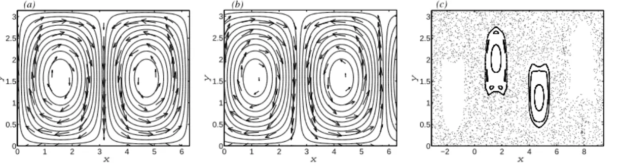
degrees of freedom. We plot in Figs. 1(a) and (b) the field lines of the alternating rolls for t = 0 and t = 3π/4 respectively and for ǫ = 0.63, and α = 0.6. The field lines which are closed curves, oscillate periodically and horizontally with a displacement of order −ǫ sin t. For ǫ = 0, the Hamiltonian is integrable, the trajectories of advected tracers coincides with streamlines. The phase space, which is here the real space, is characterized by a
chain of rolls with separatrices localized at x = mπ, with m ∈ Z. The fluid is limited
by two invariant surfaces y = π and y = 0 corresponding to the top and bottom roll boundaries. In the integrable case, as mentioned in Ref. [8], the flow is characterized by hyperbolic fixed points along the two invariant surfaces y = π and y = 0 and localized in
x = mπ, m ∈Z. These points are joined by a vertical heteroclinic connection for which the
stable and unstable manifold coincide. When ǫ 6= 0, the equations of motion of advected tracers give rise to a non integrable Hamiltonian dynamics. The two invariant surfaces y = π and y = 0 are still invariant and the phase space is now characterized by regular trajectories in the center of the rolls and a chaotic region around and between the rolls. Tracers within the center of the rolls remain confined contrary to the ones in the chaotic sea which are advected unboundedly along the channel.
A Poincar´e section of the dynamics of the stream function (1) is represented in Fig. 1(c), for ǫ = 0.63, and α = 0.6. We observe that for this value of α, the center of the cells is a regular region (characterized by quasi-periodic orbits) and chaotic advection is localized between and around these rolls. When α increase, these regular orbits break up taking place to more chaotic transport of advective particles.
Under the perturbation, i.e. for ǫ 6= 0, the vertical heteroclinic connection breaks down and the stable and unstable manifolds intersect transversely thus generating chaotic ad-vection of passive tracers [8].
The main observation is that the regular patterns persist and chaos or mixing is not well developed, the particules being spread along the channel due to chaotic transport. For that, we propose to suppress chaotic transport along the channel by creating barriers between the roll chains, and enhance the mixing within the chain. These barriers will be created around the broken separatrices of the integrable case.
We want to transform the stream function so that the mixing is enhanced within an area limited by the created barriers which prevent diffusion.
The modified stream function is otained by adding to the integrable stream function
Ψ0 = α sin x sin y,
a perturbation to the action variables of the stream function, i.e.:
Ψc(x, y, t) = α sin(x + f (y, t)) sin y. (2)
3
Construction of the perturbation
In what follows, we propose to add a perturbation f to the stream function Ψ0, which
depends on y and t, and such that the transformed stream function (2) has the following properties: the chaotic transport is confined by impenetrable barriers and a good mixing
is obtained in each of the cells bounded by these barriers.
In order to built these barriers, we first briefly summarize a method of so called parametric control.
3.1 Parametric control
Consider a Hamiltonian of the form:
H(A, θ) = H0(A) + V (A, θ),
where (A, θ) ∈ RL × TL are the action-angle variables, H0 is the integrable part and
V the perturbation. In the absence of the pertubation, the motion of the Hamiltonian
H = H0(A), which depends only on actions, is completely regular and all the orbits lie on
invariant tori with frequency vector ω = ∂H0/∂A. By adding the perturbation, the phase
space is generically made up of a mixture between regular and chaotic motions. Our aim is to derive a control term such that, for the controlled Hamiltonian
Hc(A, θ) = H0(A) + V (A + f, θ), (3)
invariant tori which act as barriers to diffusion for L = 2 are present.
Without loss of generality, we consider a region near a constant value of the action A = A0
and we set the average of V (A0, θ) to zero, i.e.
R
TLV (A0, θ)dLθ = 0. Since for sufficently
large amplitude of the perturbation the invariant torus localized at A = A0 for the
integrable part is broken, the strategy is to add a control term in the action variables
depending on angle variables which allow us to reconstruct a torus around A = A0. For
this purpose, we define the linear operator Γ as a pseudo-inverse of ω · ∂θ i.e. acting on
V =PkVkeiθ·k as Γ V = X ω·k6=0 Vk iω · ke iθ·k,
and ∂θ denotes the first derivatives of V with respect of θ. Then we translate the action
variables by a term of the form Γ ∂θV (A0, θ) so that the controlled Hamiltonian Hc
expressed in new coordinates is such that
∀θ ∈TL, Hc(A0, θ) = 0.
This requirement ensures the existence of a barrier since it implies dA/dt = 0, at A = A0.
The control term is given by:
f(θ) = Γ ∂θV (A0, θ). (4)
Using this control term, Hamiltonian (3) has an invariant torus whose equation is given
4 T.Benzekri et al
3.2 Application to the model
In order to built a barrier for the stream function (2) , we can choose a surface which is
located around x = x0 where x0 ∈ πZ. In what follows, we select x0 = 0.
The autonomous streamfunction of the model is
H(x, E, y, τ ) = E + Ψ (x, y, τ ) = ω · A + V (A, θ), where A = (x, E) are the actions, θ = (y, τ ) the angles and ω = (0, 1).
Since Ψ does not depends on E, the perturbation f is added only to x and it is given by:
f (y, τ ) = ǫ sin τ + Γ ∂yΨ (0, y, τ ) = ǫ sin τ + α cos yCǫ(τ ), (5)
where Cǫ(τ ) = Γ sin(ǫ sin τ ) = −2 X n≥0 1 2n + 1J2n+1(ǫ) cos(2n + 1)τ, (6)
and Jl for l ∈N, are Bessel functions of the first kind.
The modified stream function is then given by :
Ψc(x, y, τ ) = α sin[x + ǫ sin τ + α cos yCǫ(τ )] sin y, (7)
which has the invariant torus:
x = −α cos yCǫ(τ ), (8)
and acts as a barrier to diffusion since Hamiltonian system (7) has two degrees of freedom. We notice that y = 0 and y = π are still boundaries for the stream function (7). This comes from the fact that the perturbation does only modify the actions.
3.3 Numerical results
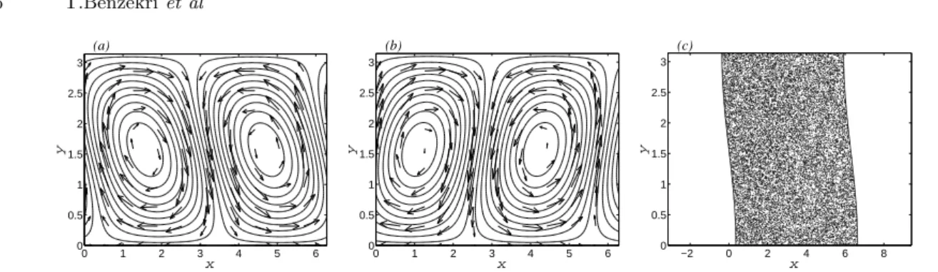
In Fig. 2(a) and (b), we depict the streamlines for Ψc given by Eq. (7). The streamlines of
the alternating rolls are slightly deformed (non-uniformly in y). Moreover, the displace-ment of these rolls remains parallel to the x-axis as it is for the stream function Ψ . But, the dynamics of tracers is completely different. For the same value of ǫ and α as in Fig. 1(c),
a Poincar´e section of the dynamics of the modified stream function Ψc given by Eq. (7) is
represented in Fig. 2(c). We notice that the perturbation which creates invariant surfaces around x = 0 (mod 2π) ( bold curves) suppresses the chaotic advection. At the same time, we observe that inside the cell bounded by the two barriers, more chaotic mixing appears: the regular trajectories observed for the streamfunction Ψ are broken by the perturbation. It means that, f (Eq. (5)) creates two invariant surfaces around x = 0 and x = 2π, and destabilises the inside of the cell and in particular the remainders of the regular motion near x = π/2 and x = 3π/2.
In order to get some clues on the origin of mixing enhancement, we compute the
Mel-nikov function. We perform the canonical transformation (x, y) 7→ (x′, y′) generated by
F2(y, x′, t) = yx′− Γ Ψ0(Φ(t), y). In the case of Ψ0, the stream function becomes
˜
Ψp(x′, y′, t) = α[sin(x′+ Φ(t)) − sin(Φ(t))] sin y′.
The Poisson bracket between Ψ0 and ˜Ψp is given by
{Ψ0, ˜Ψp} = α
2
(1 − cos x) sin(Φ(t)) sin y cos y.
It is straightforward to see that the Melnikov function vanishes when x = 0 mod 2π, i.e. on the boundaries of the cell, and is maximum (in absolute value) when x = π mod 2π, i.e. in the middle of the cell. Therefore it is expected that the mixing is enhanced since then, there is a maximum flux inside the cell [10].
In order to test the robustness of the perturbation, we simplified it.
For ǫ < 1, we can get a simplified perturbation by considering the first term of the series
Cǫ(τ ) in Eq. (6) which is given by:
fs(y, τ ) = −2αJ1(ǫ) cos y cos τ. (9)
Taking this into account, we obtain for the stream function:
Ψc(x, y, τ ) = α sin(x + ǫ sin τ − 2αJ1(ǫ) cos y cos τ ) sin y. (10)
We performed a Poincar´e section for the simplified perturbed stream function given by Eq. (10), for α = 0.6 and ǫ = 0.63. We obtain the same figure as in Fig. 2(c) with just few advected tracers showing that the simplified perturbation remains efficient.
0 1 2 3 4 5 6 0 0.5 1 1.5 2 2.5 3 x y (a) 0 1 2 3 4 5 6 0 0.5 1 1.5 2 2.5 3 x y (b) −2 0 2 4 6 8 0 0.5 1 1.5 2 2.5 3 x y (c)
Fig. 1.Streamlines at (a) t = 0 and (b) t = 3π/4, and (c) Poincar´e section of the stream function Eq. (1). The parameters are α = 0.6 and ǫ = 0.63.
4
Conclusion
We have constructed a perturbation for a model of time-dependent oscillating vortex chain for which we observe chaotic advection. By adding the suitable perturbation, we
6 T.Benzekri et al 0 1 2 3 4 5 6 0 0.5 1 1.5 2 2.5 3 x y (a) 0 1 2 3 4 5 6 0 0.5 1 1.5 2 2.5 3 x y (b) −2 0 2 4 6 8 0 0.5 1 1.5 2 2.5 3 x y (c)
Fig. 2.Streamlines at (a) t = 0 and (b) t = 3π/4, and (c) Poincar´e section of the stream function Eq. (7). The parameters are α = 0.6 and ǫ = 0.63.
obtained an efficient mixing by trapping passive tracers inside a cell while maintaining the oscillations of the rolls. With this perturbation which modifies the time-depending forcing, one is able to destroy the tori located in the center of the cells while creating barriers which suppress the chaotic diffusion along the channel.
References
1. H. Aref, Stirring by chaotic advection, J. Fluid Mech., 143 , 1 (1984).
2. J.M. Ottino, The Kinematics of mixing: streching, chaos, and transport Cambridge U.P., Cambridge, 1989. 3. R.P. Behringer , S. Meyers and H. Swinney, Chaos and mixing in geostrophic flow, Phys. Fluids A,
3, 1243 (1991).
4. M.G. Brown, K.B. Smith, Ocean stirring and chaotic low-order dynamics, Phys. Fluids, 3, 1186 (1991). 5. T.H. Solomon, J.P. Gollub, Chaotic particle transport in Rayleigh-B´enard convection, Phys. Rev. A,
38, 6280 (1988).
6. T.H. Solomon, N.S. Miller, C.J.L Spohn, J.P. Moeur, Lagrangian chaos: transport, coupling and phase separation, AIP Conf. Proc., 676, 195 (2003).
7. H. Willaime, O.Cardoso, P. Tabeling, Spatiotemporel intermittency in lines of vortices, Phys. Rev. E, 48, 288 (1993).
8. R. Camassa, S. Wiggins, Chaotic advection in Rayleigh-B´enard flow, Phys. Rev. A, 43, 774 (1991). 9. C. Chandre, G. Ciraolo, F. Doveil, R. Lima, A. Macor, M. Vittot, Channelling chaos by building
barriers, Phys. Rev. Lett., 94, 074101 (2005).
10. S. Balasuriya, Optimal perturbation for enhanced chaotic transport, Physica D, 202, 155 (2005). 11. T.Benzekri, C. Chandre, X. Leoncini, R. Lima, M. Vittot, Chaotic advection and targeted mixing,