HAL Id: hal-02971960
https://hal.archives-ouvertes.fr/hal-02971960
Submitted on 20 Oct 2020
HAL is a multi-disciplinary open access
archive for the deposit and dissemination of
sci-entific research documents, whether they are
pub-lished or not. The documents may come from
teaching and research institutions in France or
abroad, or from public or private research centers.
L’archive ouverte pluridisciplinaire HAL, est
destinée au dépôt et à la diffusion de documents
scientifiques de niveau recherche, publiés ou non,
émanant des établissements d’enseignement et de
recherche français ou étrangers, des laboratoires
publics ou privés.
Dynamical traceback age of the β Pictoris moving group
N. Miret-Roig, P. A. B. Galli, W. Brandner, H. Bouy, D. Barrado, J. Olivares,
T. Antoja, M. Romero-Gómez, F. Figueras, J. Lillo-Box
To cite this version:
N. Miret-Roig, P. A. B. Galli, W. Brandner, H. Bouy, D. Barrado, et al.. Dynamical traceback age of
the β Pictoris moving group. Astronomy and Astrophysics - A&A, EDP Sciences, 2020, 642, pp.A179.
�10.1051/0004-6361/202038765�. �hal-02971960�
https://doi.org/10.1051/0004-6361/202038765 c N. Miret-Roig et al. 2020
Astronomy
&
Astrophysics
Dynamical traceback age of the
β
Pictoris moving group
?
N. Miret-Roig
1, P. A. B. Galli
1, W. Brandner
2, H. Bouy
1, D. Barrado
3, J. Olivares
1, T. Antoja
4, M. Romero-Gómez
4,
F. Figueras
4, and J. Lillo-Box
31 Laboratoire d’astrophysique de Bordeaux, Univ. Bordeaux, CNRS, B18N, allée Geoffroy Saint-Hilaire, 33615 Pessac, France
e-mail: [email protected]
2 Max Planck Institute for Astronomy, Königstuhl 17, 69117 Heidelberg, Germany
3 Centro de Astrobiología (CSIC-INTA), ESAC Campus, Camino Bajo del Castillo s/n, 28692 Villanueva de la Cañada, Madrid,
Spain
4 Institut de Ciències del Cosmos, Universitat de Barcelona, IEEC, Martí i Franquès 1, 08028 Barcelona, Spain
Received 26 June 2020/ Accepted 16 July 2020
ABSTRACT
Context.The β Pictoris moving group is one of the most well-known young associations in the solar neighbourhood and several
members are known to host circumstellar discs, planets, and comets. Measuring its age precisely is essential to the study of several astrophysical processes, such as planet formation and disc evolution, which are strongly age-dependent.
Aims.We aim to determine a precise and accurate dynamical traceback age for the β Pictoris moving group.
Methods. Our sample combines the extremely precise Gaia DR2 astrometry with ground-based radial velocities measured in an
homogeneous manner. We use an updated version of our algorithm to determine dynamical ages. The new approach takes into account a robust estimate of the spatial and kinematic covariance matrices of the association to improve the sample selection process and to perform the traceback analysis.
Results.We estimate a dynamical age of 18.5+2.0−2.4Myr for the β Pictoris moving group. We investigated the spatial substructure of
the association at the time of birth and we propose the existence of a core of stars that is more concentrated. We also provide precise radial velocity measurements for 81 members of β Pic, including ten stars with the first determinations of their radial velocities.
Conclusions.Our dynamical traceback age is three times more precise than previous traceback age estimates and, more importantly,
for the first time it reconciles the traceback age with the most recent estimates of other dynamical, lithium depletion boundaries and isochronal ages. This has been possible thanks to the excellent astrometric and spectroscopic precisions, the homogeneity of our sample, and the detailed analysis of binaries and membership.
Key words. Galaxy: kinematics and dynamics – solar neighborhood – stars: kinematics and dynamics – open clusters and associations: individual: β Pictoris moving group – stars: formation
1. Introduction
Young local associations and moving groups are fundamental structures that help us to understand the stellar formation and evolution processes. They are small aggregates of stars (a few dozens) that share dynamical properties. For this reason, it is implicitly assumed that they were born at the same time and at the same place (from the same molecular cloud) and, therefore, they share the same chemical composition (de Zeeuw et al. 1999; Jayawardhana 2000). Most of the known associations are located nearby and allow for a detailed study of their properties.
One of the most well-known associations is β Pictoris (β Pic). It was discovered a couple of decades ago when Barrado y Navascués et al. (1999) identified the first two companions to the β Pic star and Zuckerman et al.(2001) identified an addi-tional set of 17 co-moving stars. Since then, many studies have contributed to increase the number of members of this associa-tion (e.g.Torres et al. 2006;Malo et al. 2013;Binks et al. 2015; Riedel et al. 2017b). Today, there are a few hundreds of can-didate members of the β Pic moving group, making it one of the richest associations. Its proximity (∼40 pc) and observational characteristics (it is visible both from the southern and northern
? The radial velocities are only available at the CDS via
anony-mous ftp to cdsarc.u-strasbg.fr(130.79.128.5) or viahttp:
//cdsarc.u-strasbg.fr/viz-bin/cat/J/A+A/642/A179
hemispheres) facilitated the discovery of members with a large diversity of stellar masses and very interesting properties, such as discs, confirmed exoplanets, and exocomets (Kalas & Jewitt 1995; Kalas et al. 2004; Lagrange et al. 2010,2019; Chauvin et al. 2012;Kiefer et al. 2014).
The age is one of the most fundamental parameters to study stellar formation and evolution. β Pic has an estimated age of ∼20 Myr (Barrado y Navascués et al. 1999;Barrado y Navascúes 2001;Mamajek & Bell 2014;Binks & Jeffries 2014), which is of particular interest for the study of several astrophysical pro-cesses, such as disc evolution and planet formation. However, different methods lead to a relatively broad range of values and errors ranging from 10.8 Myr to 40 Myr (see Table6for a review of the literature age estimates of β Pic).
Among the few techniques available to determine stellar ages, dynamical ages1have the advantage that they are indepen-dent of stellar evolutionary models. The main assumption of this method is that the stars were formed together, in the past, at a time when the association was most concentrated. This assump-tion is supported by the lithium and isochronal ages where there is no evidence of a significant age spread (Mamajek & Bell 2014;Messina et al. 2016). Several authors in the literature have used different techniques to traceback the positions and motions of the stars (linear trajectories, epicyclic approximation, orbital
1 The term “kinematical ages” is sometimes used for similar purposes.
Open Access article,published by EDP Sciences, under the terms of the Creative Commons Attribution License (https://creativecommons.org/licenses/by/4.0),
integration with a Galactic potential) and different definitions of the size of the association (e.g. standard deviation of the positions in a privileged direction, in 3D, maximum distance between members, pairwise encounters). Historically, the main limitations of the traceback analysis were the observational uncertainties in proper motions and the lack of trigonometric parallaxes and radial velocities to derive distances and spatial velocities (Ortega et al. 2002,2004;Song et al. 2003). After the Gaia Data Release 2 (DR2, Gaia Collaboration 2016,2018a) we have a large, uniform sample of stars with extremely pre-cise parallax and proper motions. Additionally, several authors measured radial velocities of β Pic members (e.g. Torres et al. 2006; Shkolnik et al. 2012;Gagné & Faherty 2018), although these are highly inhomogeneous and systematic errors may exist between different studies. Currently, the main limitations of the traceback analysis are: (1) the availability of an homogeneous and precise dataset of radial velocities; (2) the design of a new strategy for the selection of kinematic members adequate for the high-quality data at hand, and (3) a statistically robust approach for analysing the orbits and to establish a dynamical traceback age. In this study, we made a special effort to prepare a clean sample with precise and uniform data.
This work is structured as follows. In Sect.2, we present the spectroscopic observations we carried out and the process for measuring precise radial velocities for new and archival data. We also describe the improvements of our method for selecting a bona fide sample of kinematic members from our initial list of candidates from the literature. In Sect.3, we describe the algo-rithm used to derive the dynamical age and analyse in detail the orbits of the bona fide members. In Sect.4, we discuss the results obtained and we present our conclusions in Sect.5.
2. Data and sample selection
In this section, we present a compilation of confirmed mem-bers and new candidates reported in the literature over the past decade. In order to have a sample with homogeneous stellar parameters, we use the 5D astrometric solution (positions, par-allaxes, and proper motions) of the Gaia DR2 catalogue. We complement these data with a set of radial velocities (from our own observations plus archival data) analysed using the same methodology. In this study we use the radial velocities published in the literature and in Gaia DR2 only to compare with our own determinations. In Table1, we review the selection process from the initial compilation to the final sample.
Our initial sample is based onTorres et al.(2008),Schlieder et al.(2012),Malo et al. (2013,2014a),Gagné et al.(2015a,b, 2018),Alonso-Floriano et al.(2015),Messina et al.(2017) and Gagné & Faherty(2018). This results in a sample of 236 stars after removing the sources in common between the studies. Binaries and multiple systems are counted as one single object unless they have been resolved in previous studies. These authors used different algorithms based on the kinematics (and included the photometry in some cases) to identify new candidates or confirm members of β Pic. Most of these studies are pre-Gaia or were carried with partial information (missing parallaxes or radial velocities). For this reason, it has been necessary to develop a tool to reject kinematic outliers with our homogeneous and precise astrometry and spectroscopy (see Sect.2.3). 2.1. Proper motions and parallaxes
We use the proper motions and parallaxes of the Gaia DR2 catalogue which constitute the most recent and precise
astro-metric measurements available to date for our sample. To iden-tify the Gaia DR2 counterparts of the stars in our sample we used the 2MASS source identifier (which are given in the original tables used to construct our initial sample) and the TMASS_BEST_NEIGHBOUR table available in the Gaia archive. For 42 sources we did not find a counter part with this proce-dure, so we manually refine the match considering position and magnitude. Finally, we find proper motions and parallaxes for 222 stars in our initial sample. There are eight sources in Gaia DR2 with only the two-parameter solution and six that are not in Gaia DR2 (see AppendixA). The median of the uncertainties of this sample are ∼0.1 mas yr−1in proper motions and 0.08 mas in parallax which lead to a median error in tangential velocity of 0.19 km s−1, obtained by taking into account the correlations among the astrometric parameters (see Table1).
2.2. Radial velocities
The scarcity and quality of the radial velocities of β Pic stars are currently two of the main limitations for deriving an accurate estimate of the dynamical age of the association. Even though many radial velocity measurements are available in the litera-ture (e.g.Torres et al. 2006;Kharchenko et al. 2007;Shkolnik et al. 2012;Elliott et al. 2014;Gagné & Faherty 2018), we resort to a re-analysis of the spectra available in public archives to ensure that all the radial velocities are derived using the same methodology. The consistency and homogeneity of the individ-ual measurements is indeed particularly important in a dynami-cal traceback analysis (see e.g.Miret-Roig et al. 2018).
2.2.1. New spectroscopic observations
We performed spectroscopic observations of β Pic stars with three different instruments. The FEROS spectrograph (Kaufer et al. 1999) mounted on the ESO/MPG 2.2 m telescope operated at La Silla (Chile) was used to collect the spectra of 43 stars as part of programme 103.A-9009 (PI: W. Brandner). These obser-vations were performed in OBJCAL mode that allows for simul-taneous acquisition of the target spectrum and the calibration lamp during July and August 2019. We observed 8 stars with the CAFE spectrograph (Aceituno et al. 2013;Lillo-Box et al. 2020) mounted on the 2.2 m telescope of the Calar Alto Obser-vatory (programme: H18-2.2-015, F19-2.2-002, PI: D. Barrado). The observations were carried out from July to October 2018, right after the upgrade of the instrument. The data were pro-cessed using the new instrument pipeline described inLillo-Box et al.(2020), which performs the basic reduction and extracts the radial velocities. Finally, another 14 stars were observed with the SOPHIE spectrograph (Perruchot et al. 2008) mounted on the 1.93 m telescope of the Haute-Provence Observatory (pro-grammes: 2018A-PNPS005, 2019A-PNPS008, PI: H. Bouy). These spectra were obtained in August 2018 and May 2019 and were processed with the instrument standard data reduction pipeline which measures radial velocities by numerical cross-correlation techniques. The median signal-to-noise ratio (S/N) of our observations is 25.
2.2.2. Spectroscopic archival data
In addition to the observations conducted by our team we did an exhaustive search for the spectra available in public archives. As shown in Table 2, a total of 582 spectra have been col-lected from the European Southern Observatory (ESO) and the ELODIE archives. We reanalysed all these data (see Sect.2.2.3)
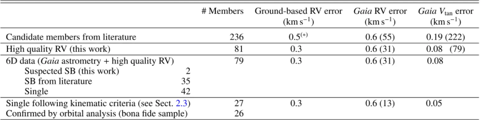
Table 1. Number of sources at each step of the data selection process (see Sect.2).
# Members Ground-based RV error GaiaRV error Gaia Vtanerror (km s−1) (km s−1) (km s−1)
Candidate members from literature 236 0.5(∗) 0.6 (55) 0.19 (222)
High quality RV (this work) 81 0.3 0.6 (31) 0.08 (79)
6D data (Gaia astrometry+ high quality RV) 79 0.3 0.6 (31) 0.08
Suspected SB (this work) 2
SB from literature 35
Single 42
Single following kinematic criteria (see Sect.2.3) 27 0.3 0.6 (13) 0.05
Confirmed by orbital analysis (bona fide sample) 26
Notes. Columns 3–4 indicate the median radial velocity error obtained from ground-based surveys and from the Gaia DR2 catalogue, respectively. For comparison, in Col. 5 we indicate the median tangential errors obtained with the Gaia DR2 parallaxes and proper motions, obtained taking into account the correlation among the astrometric parameters. The number of Gaia sources used to estimate the median velocity errors is indicated in brackets in each case.(∗)Median radial velocity errors published in the literature for the 137 stars with radial velocity previous to this work. This
sample is inhomogeneous and may be affected by systematic errors among different studies.
Table 2. Spectra analysed in this study from our spectroscopic observa-tions plus archival data.
Spectrograph R ∆λ # Spectra
(nm) Total/this work
FEROS 48 000 350–920 167/45 HARPS 115 000 378–691 138/0 ELODIE 45 000 385–680 45/0 SOPHIE 75 000 387–694 62/62 UVES 110 000 300–1100 277/0 CAFE 62 000 407–925 34/34
Notes. Number of spectra analysed and number of new spectra obtained in this study with different instruments. The total number of spectra analysed is 723 and 141 of them are new. The (maximum) resolving power and spectral range of each spectrograph are indicated.
and provide radial velocities for a larger number of stars. Table2 shows the instruments that have been used in this study and the respective number of spectra analysed in each case. We specify the number of new spectroscopic observations presented in this work (see Sect.2.2.1) which constitute a 20% of all the spec-tra. We note that some sources have been observed several times with the same or various instruments. In fact, the 723 spectra cor-respond to 81 different stars, 54% of which have been observed once, 18% twice, and the rest three or more times. We refer to Sect. 2.2.3for a description of how we combined the different radial velocity measures for the same star.
2.2.3. Radial velocities determination
The observed and downloaded spectra were reduced using the official pipeline available for each instrument. We derived radial velocities by cross-correlating the reduced spectra of the stars with the closest mask to its spectral type. We used six dif-ferent masks of spectral types A0, F0, G2, K0, K5, and M5, along with the iSpec routines for this purpose (Blanco-Cuaresma et al. 2014; Blanco-Cuaresma 2019). This procedure follows the cross-correlation technique (Baranne et al. 1996;Pepe et al. 2002) and fits a Gaussian profile to the cross-correlation function (CCF) to derive the radial velocity and associated uncertainty. We discard the radial velocity measurements resulting from a
poor fit to the CCF due to, for example, a low S/N of the spec-trum or a mismatch between the spectral type of the star and the adopted mask. We used the effective temperatures given in GaiaDR2 as a rough estimate of the spectral type of the star to choose the corresponding mask. For each star, we compute the radial velocity scatter from the results obtained with three di ffer-ent masks: the closest mask (M) to the spectral type of the star, one before (M−1), and one after (M+1). We add this number in quadrature to the formal uncertainty returned from the iSpec routines. The later step accounts for the observed fluctuation on the radial velocity results derived from different masks2.
We derive radial velocities for 81 stars of our initial sam-ple of β Pic candidates by combining our own observations with archival spectra (see Table available at CDS). In the case of mul-tiple radial velocity measurements for the same star, we proceed as follows. For each radial velocity solution (for a given star), we generate a sample of 10 000 synthetic measurements from a Gaussian distribution where the mean and variance correspond to the radial velocity and its uncertainty. We repeat this process for all radial velocity measurements of the star. Then we take the mean of the joint distribution of synthetic radial velocities as our final result for the radial velocity of the star. The uncertain-ties on the resulting radial velocity are computed from the 16% and 84% percentiles of the joint distribution of synthetic radial velocities. We note that for ten of the stars (12% of the radial velocities we determine), our radial velocity is the first measure-ment ever taken. This is an important product of our work since these data can be used to assess the membership and to study the dynamics of the association in 6D. Additionally, six of them are in our final bona fide sample of 26 stars (see Sect.2.3).
In Table 1, we compare the quality of our radial velocities with the Gaia DR2 catalogue and with previous ground-based spectroscopic surveys. We find a radial velocity in the litera-ture for 137 sources in our initial sample. These measurements come from a variety of different surveys with different quali-ties and methods to determine the radial velocity. Our measure-ments are homogeneous and about 40% more precise than this
2 This method provided an overestimate uncertainty for the β Pic star
since it is a fast rotator (v sin i = 120 km s−1, Lagrange et al. 2019)
and only the A0 mask provides reasonable CCF fit. The formal error returned by the iSpec routines is 2.2 km s−1, a 60% smaller than the
−20 −10 0 10 20 RV this work (km s−1) −6 −4 −2 0 2 4 6 R V this w ork – R V external (km s − 1) Gaia DR2 Literature
Fig. 1. Radial velocity residuals between this work and external mea-sures: Gaia DR2 (blue squares) and previous spectroscopic measures in the literature (magenta open circles). For this comparison, we used the 42 single stars with 6D data (see Table1). Our final sample of 26 stars is represented by the filled markers. We note that our radial veloc-ity uncertainties (horizontal error bars) are smaller than the markers in most of the cases. The largest uncertainty corresponds to the β Pic star (see footnote 2).
compilation which is crucial for the success of our work. We see that the radial velocities of our sample are twice as precise as the Gaia DR2 radial velocities and we have a measurement for a larger number of sources. We identified and discarded 35 sources which have been classified as binaries in previous works. In order to include the binaries in our study, we would need to determine the radial velocity motion of the centre of mass and that is beyond the scope of this work.
Figure 1 shows the comparison of the radial velocities derived in our study with the ones in Gaia DR2 and the ones in other spectroscopic surveys in the literature for the 42 sin-gle stars with 6D data in our sample. We found hints of bina-rity in two sources (2MASS J19312434-2134226 and 2MASS J22571130+3639451) and we discarded them from the analy-sis (see Appendix B). The median difference and root mean square error (RMSE) between the Gaia DR2 radial velocities and our measurements are 0.7 km s−1 and 1.0 km s−1, respec-tively. These values are computed while disregarding the source with a radial velocity difference of about 5 km s−1. The Gaia DR2 radial velocity of this star is based only in two transits, which is probably the reason for its large uncertainty. If we compare the radial velocities from the literature and our sam-ple, we obtain a median difference and RMSE of 0.3 km s−1and 0.9 km s−1, respectively. Since we believe that the homogeneity and precision of our radial velocities is superior to any other sample, we only use our measurements in the current analysis. 2.3. Kinematic sample selection
In this section, we present the kinematic selection that we designed to discard kinematic outliers in our sample. Kinematic outliers in the context of the present study refer to sources with a velocity significantly different than the group, either because they are non-members or because they are variable due to multi-plicity, for example. First, we introduce the notation we adopted to refer to position and velocity coordinate systems. We used the curvilinear heliocentric coordinates (ξ0, η0, ζ0) defined inAsiain et al. (1999) to place the stars in the configuration space. This coordinate system is centred at the current position of the Sun (R = 8.4 kpc) and rotates around the Galactic centre with a
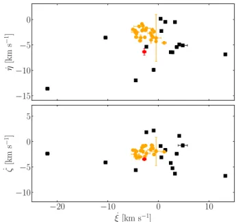
−15 −10 −5 0 ˙η [km s − 1] −20 −10 0 10 ˙ξ [km s−1] −10 −5 0 5 ˙ ζ[km s − 1]
Fig. 2.Present velocity distribution in the Galactic plane (top) and in the vertical plane (bottom) of the sample of 42 single sources with 6D data. The sample of 26 kinematically selected members is represented by the orange dots and the kinematically rejected sources are the black squares. The source 2MASS J11493184–7851011 (red dot) is retained by our kinematical criteria but is discarded due to its orbit (see text).
frequency of the circular velocity of ω = 28.81 km s−1kpc−1 (Irrgang et al. 2013). It has the advantage that it minimises the variation in each component of the configuration space. The radial component ξ0points towards the Galactic anti-centre, the azimuthal component η0is measured along the circle of radius R and is positive in the sense of the galactic rotation, and the vertical component ζ0 is defined positive towards the north Galactic pole. We also refer to the corresponding velocities as
˙
ξ0, ˙η0, ˙ζ0. The second reference system considered in this work is the Cartesian heliocentric system. The spatial components X, Y, Z, along with the velocity components U, V, W, are defined with X, U pointing towards the Galactic centre, Y, V towards the direction of Galactic rotation, and Z, W towards the north Galactic pole. We use a peculiar solar motion of (U , V , W )= (11.1, 12.24, 7.25) km s−1(Schönrich et al. 2010).
In Fig.2we represent the velocity distribution of the 42 sin-gle stars with Gaia astrometry and radial velocities from this work. We see that a number of sources have a significant scatter. Most of them were classified as members of β Pic with pre-Gaia astrometry or with no radial velocity information and clearly appear to be kinematic outliers with our extremely precise data. We discard the kinematic outliers in the 3D velocity distribution ( ˙ξ0, ˙η0, ˙ζ0) in a similar way to what we did inMiret-Roig et al. (2018). The major improvement is that in this work we use a robust estimator of the covariance matrix (the Minimum Covari-ance Determinant from Sklearn,Pedregosa et al. 2011) to fit the central location (µ) and the covariance matrix (Σ) of the velocity ellipsoid of the association. Then, we compute the Mahalanobis distance of each object defined as:
DM(x)= q
(x − µ)TΣ−1(x − µ). (1)
In Fig.B.1, we show the distribution of Mahalanobis distances. We use the percentile p65 to discard the kinematic outliers and retain 27 kinematic members (dots in Fig.2). This threshold is empiric and represents the best compromise between rejecting
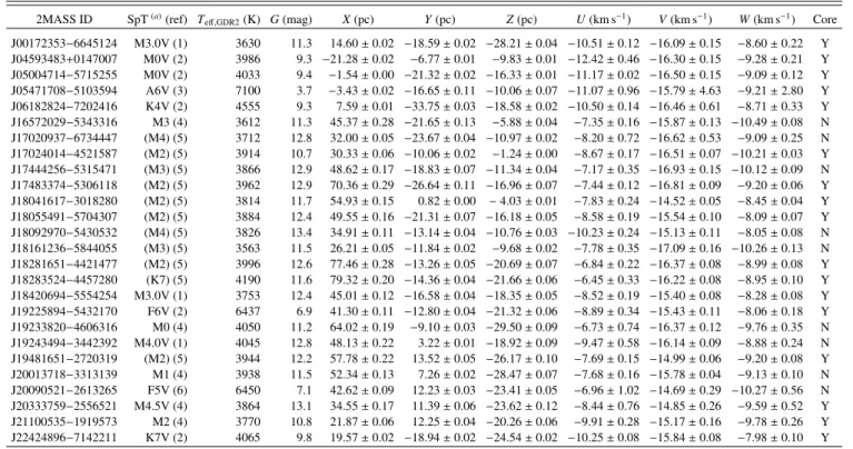
Table 3. Final bona fide sample of 26 members of β Pic selected to determine the dynamical age.
2MASS ID SpT(a)(ref) T
eff,GDR2(K) G (mag) X(pc) Y(pc) Z(pc) U(km s−1) V(km s−1) W(km s−1) Core
J00172353−6645124 M3.0V (1) 3630 11.3 14.60 ± 0.02 −18.59 ± 0.02 −28.21 ± 0.04 −10.51 ± 0.12 −16.09 ± 0.15 −8.60 ± 0.22 Y J04593483+0147007 M0V (2) 3986 9.3 −21.28 ± 0.02 −6.77 ± 0.01 −9.83 ± 0.01 −12.42 ± 0.46 −16.30 ± 0.15 −9.28 ± 0.21 Y J05004714−5715255 M0V (2) 4033 9.4 −1.54 ± 0.00 −21.32 ± 0.02 −16.33 ± 0.01 −11.17 ± 0.02 −16.50 ± 0.15 −9.09 ± 0.12 Y J05471708−5103594 A6V (3) 7100 3.7 −3.43 ± 0.02 −16.65 ± 0.11 −10.06 ± 0.07 −11.07 ± 0.96 −15.79 ± 4.63 −9.21 ± 2.80 Y J06182824−7202416 K4V (2) 4555 9.3 7.59 ± 0.01 −33.75 ± 0.03 −18.58 ± 0.02 −10.50 ± 0.14 −16.46 ± 0.61 −8.71 ± 0.33 Y J16572029−5343316 M3 (4) 3612 11.3 45.37 ± 0.28 −21.65 ± 0.13 −5.88 ± 0.04 −7.35 ± 0.16 −15.87 ± 0.13 −10.49 ± 0.08 N J17020937−6734447 (M4) (5) 3712 12.8 32.00 ± 0.05 −23.67 ± 0.04 −10.97 ± 0.02 −8.20 ± 0.72 −16.62 ± 0.53 −9.09 ± 0.25 N J17024014−4521587 (M2) (5) 3914 10.7 30.33 ± 0.06 −10.06 ± 0.02 −1.24 ± 0.00 −8.67 ± 0.17 −16.51 ± 0.07 −10.21 ± 0.03 Y J17444256−5315471 (M3) (5) 3866 12.9 48.62 ± 0.17 −18.83 ± 0.07 −11.34 ± 0.04 −7.17 ± 0.35 −16.93 ± 0.15 −10.12 ± 0.09 N J17483374−5306118 (M2) (5) 3962 12.9 70.36 ± 0.29 −26.64 ± 0.11 −16.96 ± 0.07 −7.44 ± 0.12 −16.81 ± 0.09 −9.20 ± 0.06 Y J18041617−3018280 (M2) (5) 3814 11.7 54.93 ± 0.15 0.82 ± 0.00 − 4.03 ± 0.01 −7.83 ± 0.24 −14.52 ± 0.05 −8.45 ± 0.04 Y J18055491−5704307 (M2) (5) 3884 12.4 49.55 ± 0.16 −21.31 ± 0.07 −16.18 ± 0.05 −8.58 ± 0.19 −15.54 ± 0.10 −8.09 ± 0.07 Y J18092970−5430532 (M4) (5) 3826 13.4 34.91 ± 0.11 −13.14 ± 0.04 −10.76 ± 0.03 −10.23 ± 0.24 −15.13 ± 0.11 −8.05 ± 0.08 N J18161236−5844055 (M3) (5) 3563 11.5 26.21 ± 0.05 −11.84 ± 0.02 −9.68 ± 0.02 −7.78 ± 0.35 −17.09 ± 0.16 −10.26 ± 0.13 N J18281651−4421477 (M2) (5) 3996 12.6 77.46 ± 0.28 −13.26 ± 0.05 −20.69 ± 0.07 −6.84 ± 0.22 −16.37 ± 0.08 −8.99 ± 0.08 Y J18283524−4457280 (K7) (5) 4190 11.6 79.32 ± 0.20 −14.36 ± 0.04 −21.66 ± 0.06 −6.45 ± 0.33 −16.22 ± 0.08 −8.95 ± 0.10 Y J18420694−5554254 M3.0V (1) 3753 12.4 45.01 ± 0.12 −16.58 ± 0.04 −18.35 ± 0.05 −8.52 ± 0.19 −15.40 ± 0.08 −8.28 ± 0.08 Y J19225894−5432170 F6V (2) 6437 6.9 41.30 ± 0.11 −12.80 ± 0.04 −21.32 ± 0.06 −8.89 ± 0.34 −15.43 ± 0.11 −8.06 ± 0.18 Y J19233820−4606316 M0 (4) 4050 11.2 64.02 ± 0.19 −9.10 ± 0.03 −29.50 ± 0.09 −6.73 ± 0.74 −16.37 ± 0.12 −9.76 ± 0.35 N J19243494−3442392 M4.0V (1) 4045 12.8 48.13 ± 0.22 3.22 ± 0.01 −18.92 ± 0.09 −9.47 ± 0.58 −16.14 ± 0.09 −8.88 ± 0.24 N J19481651−2720319 (M2) (5) 3944 12.2 57.78 ± 0.22 13.52 ± 0.05 −26.17 ± 0.10 −7.69 ± 0.15 −14.99 ± 0.06 −9.20 ± 0.08 Y J20013718−3313139 M1 (4) 3938 11.5 52.34 ± 0.13 7.26 ± 0.02 −28.47 ± 0.07 −7.68 ± 0.16 −15.78 ± 0.04 −9.13 ± 0.10 N J20090521−2613265 F5V (6) 6450 7.1 42.62 ± 0.09 12.23 ± 0.03 −23.41 ± 0.05 −6.96 ± 1.02 −14.69 ± 0.29 −10.27 ± 0.56 N J20333759−2556521 M4.5V (4) 3864 13.1 34.55 ± 0.17 11.39 ± 0.06 −23.62 ± 0.12 −8.44 ± 0.76 −14.85 ± 0.26 −9.59 ± 0.52 Y J21100535−1919573 M2 (4) 3770 10.8 21.87 ± 0.06 12.25 ± 0.04 −20.26 ± 0.06 −9.91 ± 0.28 −15.17 ± 0.16 −9.78 ± 0.26 Y J22424896−7142211 K7V (2) 4065 9.8 19.57 ± 0.02 −18.94 ± 0.02 −24.54 ± 0.02 −10.25 ± 0.08 −15.84 ± 0.08 −7.98 ± 0.10 Y
Notes.(a)Spectral types between parentheses were estimated from the absolute Gaia G-band magnitude.
References. (1)Riedel et al.(2017a); (2)Torres et al.(2006); (3)Gray et al.(2006); (4)Riaz et al.(2006); (5)Gagné & Faherty(2018); (6)Houk
(1982).
kinematic outliers which hinder the traceback analysis and keep-ing kinematic members in the final sample. When we compute the orbits of our targets (see Sect.3.1) we immediately see that one of them (2MASS J11493184–7851011, red circle in Fig.2) has an orbit that is significantly different from the main group and thus, we discard this object. This star has a kinematics simi-lar to β Pic but it is at >3σ in positions with respect to β Pic. We also checked that this object has the largest Mahalanobis distance to the centre of the velocity distribution. We refer to AppendixBfor a detailed discussion, source-by-source, of the kinematically rejected sources. The final sample contains 26 bona fide members of β Pic and their 3D positions and veloc-ities are given in Table3.
2.4. Bona fideβ Pic sample
In this paper, we make a substantial effort to prepare a robust sample of β Pic members with the best precision possible in their determination of the positions in the 6D space phase. Then we used this valuable data to identify and remove kinematic outliers. In this section, we review the main characteristics of our final sample.
The relative error in the parallax of these members is less than 1% which allows us to compute the distance as the inverse of parallax. We note that four stars have a parallax error <0.1% at distances up to 50 pc. The median relative errors in proper motions are of 0.3% in right ascension (µα∗) and 0.09% in
decli-nation (µδ). The precision in µα∗and µδis similar but a few
mem-bers have µα∗ close to zero which increases the relative error.
The β Pic star is the brightest source (G = 3.7 mag) and causes a fraction of the pixel used in the standard Gaia DR2 analysis to be saturated. Hence, measurements of its centroid position and
the resulting astrometry are less precise than for fainter sources (G > 6 mag) (Lindegren et al. 2018).
In Table4, we provide the median heliocentric position and velocity of β Pic. We see that the observational uncertainties in positions (σerr) are of the order of tenths of parsecs and thus, the observed dispersion (σobs) can be interpreted as an intrin-sic dispersion (σint). The dispersion in the Galactic plane (X, Y components) is twice the vertical dispersion (Z). When we look at the velocity dispersion, we find that the median errors in velocity (σerr) are significantly smaller than the velocity dis-persion observed (σobs), indicating the presence of an intrinsic cosmic dispersion (σint). Therefore, the dispersion we observe in Fig. 2 is intrinsic and not due to observational errors. The velocity ellipsoid is elongated in the radial direction (towards the Galactic centre) with a dispersion that is twice that of those in the other two directions. The typical velocity dispersions observed in molecular clouds are of the order of 0.5 to 1 km s−1 in nearby, low-mass star-forming regions (and references therein Hennebelle & Falgarone 2012;Heyer & Dame 2015), similar to the velocity dispersion we find in β Pic.
3. Traceback analysis
In this section, we describe our methodology to perform the traceback analysis which is based on the work ofMiret-Roig et al.(2018), with some improvements.
3.1. Towards a dynamical age estimate
We consider the same 3D Milky Way potential as inMiret-Roig et al.(2018) to integrate the equations of motion. This model is based on theAllen & Santillan(1991) potential which consists
Table 4. Parameters of the distribution in positions (in pc) and in velocities (in km s−1) of the 26 bona fide kinematic members of β Pic in the
present (t= 0 Myr).
Positions
X Y Z σobs,X σobs,Y σobs,Z σerr,X σerr,Y σerr,Z σint,X σint,Y σint,Z 47.49 −7.89 −17.92 16.04 13.18 7.44 0.11 0.04 0.05 15.93 13.14 7.39
Velocities
U V W σobs,U σobs,V σobs,W σerr,U σerr,V σerr,W σint,U σint,V σint,W
−8.74 −16.16 −9.98 1.49 0.54 0.70 0.24 0.11 0.11 1.25 0.43 0.59
Notes. Columns indicate: (1–3) central location of the distribution, (4–6) robust standard deviation, (7–9) median errors, and (10–12) a rough estimate of the intrinsic dispersion, computed as σ2
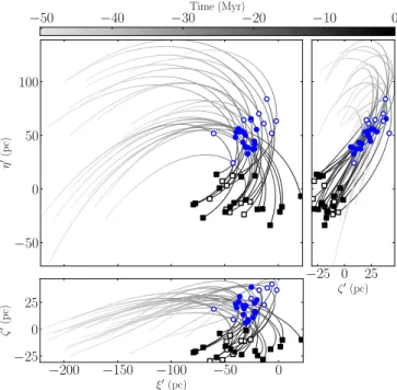
int= σ 2 obs−σ 2 err. −50 −40 −30Time (Myr)−20 −10 0 −50 0 50 100 η 0(p c) −200 −150 −100 −50 0 ξ0(pc) −25 0 25 ζ 0(p c) −25 0 25 ζ0(pc)
Fig. 3.Orbital projection in the Galactic plane (top left) and in the two vertical planes (bottom left and top right) of our bona fide sample of 26 members of β Pic, integrated back in time 50 Myr, under the new A&S potential. The orbits are colour-coded with the backwards time, the black squares represent the positions in the present (t = 0 Myr), and the blue dots represent positions at birth time (t= −18.5 Myr). The filled markers correspond to the core of β Pic defined in Sect.3.2.
of a spherical central bulge, a disc, and a massive spherical halo, but with updated parameters taken from (their Table 1Irrgang et al. 2013). Hereafter we refer to this model as new A&S and we compare it with other axisymmetric models in Sect.3.3. In Fig.3, we show the 2D orbital projections in the Galactic plane and the two vertical planes of the 26 bona fide members in our sample. The orbits have been integrated back in time 50 Myr.
Following the example of other studies (e.g.Fernández et al. 2008;Ducourant et al. 2014;Mamajek & Bell 2014;Riedel et al. 2017b;Miret-Roig et al. 2018), we define the dynamical age as the time at which the members of the association were most centrated in space. The algorithm to measure the degree of con-centration, hereafter the size of the association, is of uttermost importance and different strategies to compute the size have been used in the literature. These different methodologies have signif-icantly contributed to the large spread in the dynamical trace-back ages determined. In general, the size of the association is estimated with the empiric standard deviation in the spatial
coor-dinates. However, it is very sensitive to the presence of outliers, i.e. members which significantly deviate from the mean posi-tion of the associaposi-tion which are not necessarily contaminants. In this section, we present three strategies to estimate the size of the association as a function of time. Some of them are based on classical functions used in the literature (i.e. the variance) and others are novel, representing the overall variance of the associ-ation, and independent of the coordinates chosen. In the follow-ing, we define the three functions we use to estimate the size of the association in a way that they all have units of length.
– The size in the radial, azimuthal, and vertical directions (Sξ0,
Sη0, Sζ0) are the squared root of the diagonal terms of the
covariance matrix in each direction.
– The Trace Covariance Matrix Size (STCM) is defined as: STCM=
" Tr(Σ) 3
#1/2
. (2)
– The Determinant Covariance Matrix Size (SDCM) is defined as:
SDCM= [det(Σ)]1/6. (3)
Each of these expressions are computed from the covariance matrix of the association in the configuration space. We used two different algorithms to estimate the covariance matrix, namely the empirical covariance estimation, and the robust covariance estimation, both from the Sklearn packages (Pedregosa et al. 2011). Whereas the first corresponds to the classical maximum likelihood estimator, the second is less sensitive to outliers in the dataset.
The size estimators Sξ0, Sη0, and Sζ0, when computed with
the empirical covariance estimation, correspond to the classical standard deviation in each direction. The other two size estima-tors (STCMand SDCM) can be interpreted from the eigenvalues of the covariance matrix. The trace of the association, often referred as the total variance of the covariance matrix, coincides with the sum of its eigenvalues. In Eq. (2), we introduce a factor of 1/3 (in a 3D space) so that we can interpret the STCMestimator as the arithmetic mean of the variances in the individual components. In any case, this multiplicative factor changes the absolute value of the size estimator but not the locus of the minimum, which is our main interest. The determinant of the covariance matrix, also known as the generalised variance, can be interpreted as the geo-metric mean of the eigenvalues of the covariance matrix. Then, the volume of the association is proportional to the squared root of the determinant of the covariance matrix. Finally, we define the diagonal of the Determinant Covariance Matrix Size (SdDCM) analogously to the SDCMsize but only considering the diagonal terms, that is, neglecting the correlations among the three spa-tial components. This is not a good estimator of the size of the
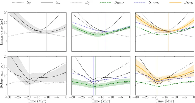
0 5 10 15 20 Empiric size (p c) −30 −25 −20 −15 −10 −5 0 Time (Myr) 0 5 10 15 20 Robust size (p c) −30 −25 −20 −15 −10 −5 0 Time (Myr) −30 −25 −20 −15 −10 −5 0 Time (Myr) Sξ0 Sη0 Sζ0 SDCM SdDCM ST CM
Fig. 4.Size of the β Pic association as a function of backwards time computed with the empirical covariance estimate (top panels) and the robust covariance estimate (bottom panels). The association size estimates considered in this study are indicated in the legend and described in the text. The lines represent the median of 1000 bootstrap repetitions and the shaded areas represent the 1σ uncertainties. The orbits were integrated using the new A&S potential.
association since it neglects part of the information included in the covariance matrix. However, it can be understood as a geo-metric mean of the size estimators Sξ0, Sη0, Sζ0, so we include it
only for comparison.
In Fig.4we show the six parameters defining the size of β Pic (Sξ0, Sη0, Sζ0, SDCM, SdDCM, STCM) computed with the
empiri-cal covariance estimate and the robust covariance estimate as a function of time. It is remarkable that the minimum size obtained with the empirical covariance estimate (top panels) depends on the size estimator, whereas we find a minimum at a similar times for all the size estimators considered with the robust covariance estimate (bottom panels). This is because the robust covariance estimate gives less weight to sources with a large dispersion, attenuating the impact of outliers.
Going forward, we only considered the size estimates com-puted with the robust covariance estimates. In the left bottom panel of Fig.4, we show the dispersion in the radial, azimuthal, and vertical direction, independently. We see that the vertical component does not provide useful information for constrain-ing the age of the association, while the two components in the Galactic plane have a minimum at a similar time. In this panel we highlighted the azimuthal component (Sη0) which is the size
estimator we used inMiret-Roig et al.(2018).
In the middle bottom panel, we add the size from the deter-minant of the covariance matrix (SDCM) and, for comparison, the inaccurate size using only the diagonal values of this matrix (SdDCM), that is, with and without correlations, respectively. Both curves have close minima with a time difference of ∼1 Myr, and are also similar to the age obtained with the Sη0 size
esti-mator. The correlations reduce the value of the determinant and in consequence, the absolute value of SDCM, estimating a birth size of the association of ∼5 pc. In the right bottom panel, we include the size estimator from the trace (STCM). As mentioned
before, the STCM and SDCM sizes correspond to the arithmetic and geometric mean of the eigenvalues of the covariance matrix, respectively. These two statistics are related by an inequality in which the arithmetic mean is always larger than the geometric mean and they are only equal if all the individual values are the same. This corresponds to an isotropic covariance matrix, which is not the case in our study.
Currently, thanks to the excellent astrometric precision of Gaia and the homogeneous precise radial velocity sample derived in this work, the observational uncertainties are no longer what dominates the uncertainties in the dynamical age. We propagated the present uncertainties with an analytic approx-imation (Miret-Roig et al. 2018) and estimated that the disper-sion due to observational uncertainties is.2 pc at the time of minimum size. At birth, the association had a STCMsize of ∼7 pc (see Fig.4), which is similar to what has been observed in star-forming regions such as Ophiuchus (Cánovas et al. 2019), Taurus (Galli et al. 2019), and Corona Australis (Galli et al. 2020).
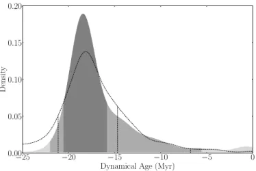
As mentioned, the sample selection (i.e. the presence of con-taminants or unidentified binaries) is extremely important. To estimate the impact of the sample selection on the age, we took 1000 random samples of the 26 bona fide β Pic members and estimated the dynamical age with each. Then, we can determine a dynamical age and a robust uncertainty from the distribution of ages. In Fig.5, we report a kernel density estimate of the age distribution with a bandwidth of 1 Myr; this value is smaller and of the order of the age uncertainties. In Table5, we report the mode and the 68%, 95%, and 99.7% highest density intervals3of
3 The highest density interval is defined such that all points within
the interval have a higher probability density than all points outside the interval. We used the ArviZ python package (Kumar et al. 2019) to compute it.
−25 −20 −15 −10 −5 0 Dynamical Age (Myr)
0.00 0.05 0.10 0.15 0.20 Densit y
Fig. 5. Dynamical age distribution of the bona fide β Pic members, obtained with the robust estimate of the covariance matrix. The dis-tribution obtained with the STCM size estimator is colour-coded with
the 68%, 95%, and 99.7% highest-density intervals. The distribution obtained with the SDCM size estimator is shown in dashed lines and
the same highest density intervals are shown. The orbits were inte-grated using the new A&S potential and we computed 1000 bootstrap repetitions.
the age distribution. Considering the STCMsize estimator and the 68% highest density interval, we find a dynamical age of β Pic of 18.5+2.0−2.4Myr (see Table5). With the SDCMsize estimator, we obtain a similar age, 17.6+3.5−2.9Myr. We note that the two values agree within a 1 Myr difference which is significantly smaller than the age uncertainty.
3.2. Signs of substructure at birth time
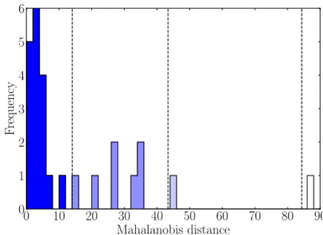
When we look at Fig.3, we see that at birth, some stars appeared to be more concentrated and forming a core (filled dots), while a few members appeared to be more dispersed (empty dots). To identify these two populations, we compute the Mahalanobis dis-tance (Eq. (1)) with the robust central location and covariance of the 3D spatial distribution (ξ0, η0, ζ0). In Fig.C.1, we show the distribution of the Mahalanobis distances. We used the percentile p68 to separate the core from the peripheral stars which results in 17 core stars and 9 peripheral stars (see Table3). These stars were selected at birth time in the space of positions and in this space they appear most concentrated (see Fig.3). Interestingly, in the present, the stars forming the core appear more dispersed than those originally more dispersed. In the velocity space, both populations are mixed in the present and at birth time.
It is worth mentioning that if we use only the 17 core stars to study the dynamical age, we obtain an age very similar to the value we obtained in Sect.3.1. With the STCMsize we find an age of 18.8+1.7−2.1Myr and with the SDCMsize an age of 17.6+3.5−1.2Myr. As expected, in this case were all the stars are well concen-trated at birth time, the age is independent of the covariance esti-mate used (empirical or robust). Additionally, the small bump we observe in Fig.6at ∼–15 Myr disappears with the age distri-bution obtained only with the 17 core stars. In short, if we use the core sample of 17 stars to trace back the age of β Pic we find variations of less than 1 Myr with respect to the value we obtained in Sect.3.1, with all the covariance and size estimates considered in this study. This is the first time that the spatial dis-tribution of β Pic is analysed in detail and these results should be revisited with a larger sample of members.
3.3. Effect of the Galactic potential
In this section, we discuss the effect of considering dif-ferent Galactic axisymmetric potentials and including non-axisymmetric structures such as spiral arms, on the dynamical age. First, we considered two additional axisymmetric poten-tials, namely the one ofMcMillan(2017, hereafter McMillan17) and the one ofBovy (2015, hereafter MWPotential14). These two models together with the new A&S model have similar rota-tion curves in the range of radius relevant here with only slight differences in the mass distribution as can be seen in their respec-tive rotation curves (Fig. D.1 inGaia Collaboration 2018bfor a comparison of new A&S and McMillan2017 and Fig. 8 inBovy 2015for MWpotential14).
We also used a non-axisymmetric potential which accounts for the spiral arms in addition to the axisymmetric potential described in Sect. 3.1. The 3D spiral model is the PERLAS spiral arms fromPichardo et al. (2003, hereafter new A&S + spiral arms (P03)). The locus is the one followingDrimmel & Spergel(2001) and has a pitch angle of 15.5◦. We take a pattern speed ofΩP = 21 km s−1kpc−1and a mass of 0.04% of the disc mass. These values are in agreement with the values proposed inAntoja et al.(2011). Recently,Eilers et al.(2020) estimated a density contrast at the solar radius of 20% which is similar to the amplitude of the arms used here which leads to a contrast of around 23% (Antoja et al. 2011).
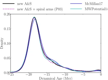
In Fig.6we present the dynamical age distribution obtained with different axisymmetric potentials and with the non-axisymmetric potential with spiral arms. In Table 5 we report the percentiles of the dynamical age distribution for each of the potentials considered. The variations in the dynamical age due to the Galactic potential are minimal, and they are all compatible with the value we obtained in Sect.3.1. Therefore, we conclude that the variations in the dynamical age produced by different Galactic potentials are much lower than our main source of uncer-tainty, that is, the membership. This is valid for the potentials we have tested, the parameters of which are constrained by recent observations of the Milky Way and can be explained for the short integration times given the low age of the association. Given that the different Galactic potentials considered here lead to changes in the dynamical age smaller than the current uncertainties, we decided to keep the results obtained with the new A&S potential which has fewer parameters.
4. Discussion
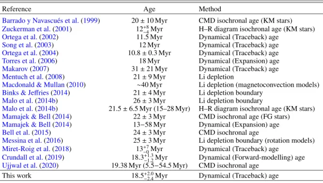
In the previous section, we discussed different strategies to deter-mine the dynamical traceback age of β Pic. All of them are com-patible, with differences of .1 Myr, significantly smaller than the age uncertainties. Going forward, we adopt the an age of 18.5+2.0−2.4Myr, obtained for the sample of 26 bona fide members, with the STCM size, and with the axisymmetric potential. Our study provides the first traceback age which conforms with other dynamical ages recently published in the literature, such as the expansion or the forward-modelling algorithms and with ages based on evolutionary models such as the lithium depletion or the isochronal ages. In Table6, we present a compilation of previous age estimates published in the literature and we see that our deter-mination is compatible with the majority of them. The first reli-able age determination of the β Pic star and its moving group was an isochronal age presented inBarrado y Navascués et al.(1999), 20 ± 10 Myr, which is in full agreement with our current estimate. The earliest traceback studies of β Pic obtained an age of 11–13 Myr (Ortega et al. 2002; Song et al. 2003; Ortega et al. 2004), which is younger that what we find here. These
Table 5. Dynamical age (in Myr) obtained with the robust metrics for different potentials.
Potential Size estimator p0.15 p2.5 p16 Mode p84 p97.5 p99.85
New A&S SDCM −32.0 −27.6 −21.1 −17.6 −14.7 −6.8 0
McMillan17 SDCM −43.9 −29.3 −20.2 −17.7 −14.6 −8.1 0
MWPotential14 SDCM −46.5 −27.8 −21.2 −17.7 −14.6 −6.1 −1.5
New A&S+ spiral arms (P03) SDCM −46.4 −29.3 −20.8 −17.9 −14.4 −7.6 0
New A&S STCM −25.2 −22.0 −20.5 −18.5 −15.9 −5.6 0
McMillan17 STCM −26.3 −22.2 −19.7 −18.2 −15.2 −8.6 0
MWPotential14 STCM −26.3 −23.7 −20.7 −18.7 −16.2 −7.6 0
New A&S+ spiral arms (P03) STCM −26.4 −22.3 −20.2 −18.5 −15.9 −5.6 0
Notes. We report the mode and the highest density interval for probabilities of 68%, 95%, and 99.7%.
−25 −20 −15 −10 −5 0
Dynamical Age (Myr) 0.00 0.05 0.10 0.15 0.20 Densit y new A&S
new A&S + spiral arms (P03)
McMillan17 MWPotential14
Fig. 6.Dynamical age distribution of β Pic obtained with the STCMsize
estimator and different axisymmetric potentials (solid lines) and with the new A&S+ spiral arms (P03) potential (dashed line).
differences are most probably due to the large observational uncertainties of the pre-Gaia astrometry and, thus, to the pres-ence of a significant number of kinematic contaminants. Those authors used the maximum size between stars to determine the age of the association. We did not consider this size estimator in our study but it is clearly sensitive to the presence of outliers in the dataset.
Miret-Roig et al.(2018) measured a dynamical age of β Pic of 13+7−0Myr with a method that is very similar to the one pre-sented in this work. We believe that the main differences between these two studies are (1) the precision of the 6D space phase positions, (2) the new sample selection based on a robust esti-mate of the 3D velocities covariance matrix, and (3) the new orbital analysis which uses an improved size estimator of the association.
In our previous study, we used the Gaia DR1 astrometry and a compilation of radial velocities from the literature without any treatment. Here, we use the improved precision of Gaia DR2 and a uniform sample of radial velocities. The median uncer-tainty in the DR1 parallaxes and proper motions were 0.3 mas and 0.2 mas yr−1, respectively, compared to the values 0.05 mas and <0.1 mas yr−1now available from the DR2. We discarded ten objects from our previous sample for being classified as binaries and five others do not have a radial velocity measurement in our work. These leaves only six objects in common between the two works (23% of our new sample). The black solid line in Fig.4
(Sη0) corresponds to the methodology used inMiret-Roig et al.
(2018, their blue curve in Fig. 7). We see that with the empiric covariance (top panel) matrix we still find younger dynamical traceback ages. On the contrary, the size estimator Sη0, if we use
a robust estimate of the covariance matrix, we recover a similar age to the one reported in Sect.3.1.
Another technique used in the literature to measure a kine-matic age consists of studying if the association is under expan-sion. Torres et al. (2006) found a linear relation between the velocity and the position in the direction of the Galactic cen-tre, which results in an age of ∼18 Myr. In a similar approach, Mamajek & Bell(2014) found an age of 21+10−5 Myr, taking into account the positions and velocities in the Galactic plane. Both results are compatible with what we obtain here. In addition, we used our new accurate sample to estimate an expansion age of β Pic. We fitted a line between the Cartesian heliocentric posi-tions XYZ and velocities UVW. We find evidence of expansion in the direction towards the Galactic centre and in the direction of Galactic rotation with slopes of κX = 0.057 ± 0.006 km s−1pc−1 and κY = 0.033 ± 0.008 km s−1pc−1, respectively. In the verti-cal direction, we find a slope of κZ = −0.02 ± 0.02 km s−1pc−1, which is slightly negative but compatible with zero. These coef-ficients result in an expansion age4of 17 ± 2 Myr and 29 ± 4 Myr in the radial and azimuthal directions. If we combine these mea-sures with a weighted mean as done byMamajek & Bell(2014), we obtain an expansion age of 20±4 Myr, in excellent agreement with our traceback age.
Recently, Crundall et al. (2019) provided a new tool (Chronostar) to determine a dynamical age applying the forward-modelling technique, and obtained an age of 18.3+1.3−1.2Myr. It is interesting to see how similar the results of their study are to ours despite the different sample of members (we have 15 members in common, 25% of their sample) and method used. These results prove that both methods are complementary. Their method allowed them to detect the β Pic members among a large catalogue of field stars while ours provides a deeper orbital anal-ysis allowing us to discover, for example, the existence of a central core and a more dispersed structure at birth time.
Finally, it is important to mention that the age estimates in the literature based on the Li depletion or isochronal fitting obtained values very similar to the one obtained here and, in gen-eral, with a lower dispersion than the dynamical age estimates obtained up to now (see Table 6). If we exclude the work of Macdonald & Mullan(2010) which obtained an age of ∼40 Myr, twice the other works, we obtain a median value of 21 ± 4 Myr
4 To compute the expansion age we used the relation τ= γ−1κ−1, where
Table 6. Literature age estimates for β Pic.
Reference Age Method
Barrado y Navascués et al.(1999) 20 ± 10 Myr CMD isochronal age (KM stars) Zuckerman et al.(2001) 12+8−4Myr H–R diagram isochronal age (KM stars)
Ortega et al.(2002) 11.5 Myr Dynamical (Traceback) age
Song et al.(2003) 12 Myr Dynamical (Traceback) age
Ortega et al.(2004) 10.8 ± 0.3 Myr Dynamical (Traceback) age
Torres et al.(2006) 18 Myr Dynamical (Expansion) age
Makarov(2007) 31 ± 21 Myr Dynamical (Traceback) age
Mentuch et al.(2008) 21 ± 9 Myr Li depletion
Macdonald & Mullan(2010) ∼40 Myr Li depletion (magnetoconvection models) Binks & Jeffries(2014) 21 ± 4 Myr Li depletion boundary
Malo et al.(2014b) 26 ± 3 Myr Li depletion boundary
Malo et al.(2014b) 21.5 ± 6.5 Myr (15–28 Myr) H–R diagram isochronal age (KM stars) Mamajek & Bell(2014) 22 ± 3 Myr CMD isochronal age (FG stars)
Mamajek & Bell(2014) 13−58 Myr Dynamical (Expansion) age
Bell et al.(2015) 24 ± 3 Myr CMD isochronal age
Messina et al.(2016) 25 ± 3 Myr Li depletion boundary (rotation models) Miret-Roig et al.(2018) 13+7−0Myr Dynamical (Traceback) age
Crundall et al.(2019) 18.3+1.3−1.2Myr Dynamical (Forward-modelling) age Ujjwal et al.(2020) 19.38 Myr (5.5−54.5 Myr) CMD isochronal age
This work 18.5+2.0−2.4Myr Dynamical (Traceback) age
Notes. This table is an udated version of Table 1 fromMamajek & Bell(2014).
which is in good agreement with the age we measured. This is an important result since our method is independent of evolutionary models and these are two very different strategies.
5. Conclusions
In this work we measured a dynamical, traceback age of the β Pic moving group of 18.5+2.0−2.4Myr which is compatible with ages based on evolutionary models. Our age estimate is the first trace-back age that reconciles the ages determined by the tracetrace-back method with other dynamical ages (expansion, forward mod-elling), lithium depletion ages, or isochronal ages.
The precision in the dynamical traceback age we achieved in this study is thanks to the combination of the Gaia DR2 astrom-etry and the uniform radial velocity sample of single stars that we produced in this work. We measured the radial velocity of 81 candidate members of β Pic in a uniform manner. For ten sources, our measure is the first radial velocity estimate. This is an important result of our work, allowing us to identify 15 kinematic outliers from our initial sample and two new potential spectroscopic binaries.
Our improved algorithm to determine the age (based on our previous work,Miret-Roig et al. 2018) provides a more rigor-ous kinematic sample selection and an improved orbital anal-ysis. We showed the importance of using a robust estimate of the covariance matrix (instead of an empirical one) to minimise the impact of outliers (sources which deviate from the central locus of the association which are not necessarily contaminants). We explored different size estimators computed from the covari-ance matrix to determine the dynamical age (the standard devi-ation in different directions, the determinant, and the trace). All of them provide dynamical ages with differences of less than 1 Myr, meaning that they are compatible within the uncertainties, when computed from the robust covariance matrix. Our thorough orbital analysis allowed us to propose the existence of a central core of 17 stars which appeared more concentrated at birth time.
In this study, we show that different potentials (i.e. axysim-metrics and including the effect of spiral arms) lead to changes in the dynamical age that are within the current uncertainties. Nowadays, the major source of uncertainty in the dynamical, traceback age is the sample selection and the errors in the radial velocity estimates. For this reason, we stress the importance of choosing samples with accurate radial velocity data, with uncer-tainties comparable to the imminent eDR3 Gaia release. This is crucial to reject kinematic contaminants and binaries and to ensure the success of a traceback analysis.
Acknowledgements. We acknowledge Ferran Torra for his advice in the proper use of Gaia DR2 data. This research has received funding from the European Research Council (ERC) under the European Union’s Horizon 2020 research and innovation programme (grant agreement No 682903, P.I. H. Bouy), and from the French State in the framework of the “Investments for the future” Pro-gram, IdEx Bordeaux, reference ANR-10-IDEX-03-02. Based in part on obser-vations made at Observatoire de Haute Provence (CNRS), France. Based on observations collected at the Centro Astronómico Hispano-Alemán (CAHA) at Calar Alto, operated jointly by Junta de Andalucía and Consejo Superior de Investigaciones Científicas (IAA-CSIC). Based on observations collected at the European Organisation for Astronomical Research in the Southern Hemi-sphere under programmes 0103.A-9009, 088.A-9007, 089.A-9007, 089.A-9013, 089.D-0709, 090.A-9010, 090.C-0200, 090.C-0815, 091.A-9012, 091.A-9013, 091.C-0216, 091.C-0595, 092.A-9002, 092.A-9009, 093.A-9006, 093.A-9029, 094.A-9002, 094.A-9012, 095.A-9029, 099.A-9005, 099.A-9029. This research has been funded by the Spanish State Research Agency (AEI) Projects No. ESP2017-87676-C5-1-R and No. MDM-2017-0737 Unidad de Excelencia “María de Maeztu”- Centro de Astrobiología (INTA-CSIC). This work was sup-ported by the MINECO (Spanish Ministry of Economy) through grant RTI2018-095076-B-C21 (MINECO/FEDER, UE). This research has made use of the SIMBAD database, operated at CDS, Strasbourg, France. This work made use of the Topcat software (Taylor et al. 2005). We acknowledge the Gaia Project Scientist Support Team and the Gaia Data Processing and Analysis Consor-tium (DPAC) for the python code PyGaia (https://github.com/agabrown/ PyGaia) The figures presented here were created using Matplotlib (Hunter 2007). TA has been funded by European Union’s Horizon 2020 research and innovation programme under the Marie Skłodowska-Curie grant agreement No. 745617.
References
Aceituno, J., Sánchez, S. F., Grupp, F., et al. 2013,A&A, 552, A31
Allen, C., & Santillan, A. 1991,Rev. Mex. Astron. Astrofis., 22, 255
Alonso-Floriano, F. J., Caballero, J. A., Cortés-Contreras, M., Solano, E., & Montes, D. 2015,A&A, 583, A85
Antoja, T., Figueras, F., Romero-Gómez, M., et al. 2011,MNRAS, 418, 1423
Asiain, R., Figueras, F., & Torra, J. 1999,A&A, 350, 434
Baranne, A., Queloz, D., Mayor, M., et al. 1996,A&AS, 119, 373
Barrado y Navascúes, D. 2001, in The β Pic Moving Group: a New Age Assesment, eds. R. Jayawardhana, & T. Greene ,ASP Conf. Ser., 244, 63
Barrado y Navascués, D., Stauffer, J. R., Song, I., & Caillault, J. P. 1999,ApJ, 520, L123
Bell, C. P. M., Mamajek, E. E., & Naylor, T. 2015,MNRAS, 454, 593
Binks, A. S., & Jeffries, R. D. 2014,MNRAS, 438, L11
Binks, A. S., & Jeffries, R. D. 2016,MNRAS, 455, 3345
Binks, A. S., Jeffries, R. D., & Maxted, P. F. L. 2015,MNRAS, 452, 173
Blanco-Cuaresma, S. 2019,MNRAS, 486, 2075
Blanco-Cuaresma, S., Soubiran, C., Heiter, U., & Jofré, P. 2014,A&A, 569, A111
Bovy, J. 2015,ApJS, 216, 29
Cánovas, H., Cantero, C., Cieza, L., et al. 2019,A&A, 626, A80
Cantat-Gaudin, T., Jordi, C., Vallenari, A., et al. 2018,A&A, 618, A93
Chauvin, G., Lagrange, A. M., Beust, H., et al. 2012,A&A, 542, A41
Crundall, T. D., Ireland, M. J., Krumholz, M. R., et al. 2019,MNRAS, 489, 3625
de Zeeuw, P. T., Hoogerwerf, R., de Bruijne, J. H. J., Brown, A. G. A., & Blaauw, A. 1999,AJ, 117, 354
Drimmel, R., & Spergel, D. N. 2001,ApJ, 556, 181
Ducourant, C., Teixeira, R., Galli, P. A. B., et al. 2014,A&A, 563, A121
Eilers, A. C., Hogg, D. W., Rix, H. W., et al. 2020, ApJ, submitted [arXiv:2003.01132]
Elliott, P., Bayo, A., Melo, C. H. F., et al. 2014,A&A, 568, A26
Fernández, D., Figueras, F., & Torra, J. 2008,A&A, 480, 735
Gagné, J., & Faherty, J. K. 2018,ApJ, 862, 138
Gagné, J., Faherty, J. K., Cruz, K. L., et al. 2015a,ApJs, 219, 33
Gagné, J., Lafrenière, D., Doyon, R., Malo, L., & Artigau, É. 2015b,ApJ, 798, 73
Gagné, J., Roy-Loubier, O., Faherty, J. K., Doyon, R., & Malo, L. 2018,ApJ, 860, 43
Gaia Collaboration (Prusti, T., et al.) 2016,A&A, 595, A1
Gaia Collaboration (Brown, A. G. A., et al.) 2018a,A&A, 616, A1
Gaia Collaboration (Helmi, A., et al.) 2018b,A&A, 616, A12
Galli, P. A. B., Loinard, L., Bouy, H., et al. 2019,A&A, 630, A137
Galli, P. A. B., Bouy, H., Olivares, J., et al. 2020,A&A, 634, A98
Gray, R. O., Corbally, C. J., Garrison, R. F., et al. 2006,AJ, 132, 161
Hartman, J. D., Bakos, G. Á., Noyes, R. W., et al. 2011,AJ, 141, 166
Hennebelle, P., & Falgarone, E. 2012,A&ARv., 20, 55
Heyer, M., & Dame, T. M. 2015,ARA&A, 53, 583
Houk, N. 1982,Michigan Catalogue of Two-dimensional Spectral Types for the HD stars. Volume 3. Declinations −40 to −26
Hunter, J. D. 2007,Comput. Sci. Eng., 9, 90
Irrgang, A., Wilcox, B., Tucker, E., & Schiefelbein, L. 2013,A&A, 549, A137
Janson, M., Durkan, S., Hippler, S., et al. 2017,A&A, 599, A70
Jayawardhana, R. 2000,Science, 288, 64
Kalas, P., & Jewitt, D. 1995,AJ, 110, 794
Kalas, P., Liu, M. C., & Matthews, B. C. 2004,Science, 303, 1990
Kaufer, A., Stahl, O., Tubbesing, S., et al. 1999,The Messenger, 95, 8
Kharchenko, N. V., Scholz, R. D., Piskunov, A. E., Röser, S., & Schilbach, E. 2007,Astron. Nachr., 328, 889
Kiefer, F., Lecavelier des Etangs, A., Boissier, J., et al. 2014,Nature, 514, 462
Klutsch, A., Freire Ferrero, R., Guillout, P., et al. 2014,A&A, 567, A52
Kraus, A. L., Herczeg, G. J., Rizzuto, A. C., et al. 2017,ApJ, 838, 150
Kumar, R., Carroll, C., Hartikainen, A., & Martin, O. A. 2019,J. Open Source Soft.
Lagrange, A. M., Bonnefoy, M., Chauvin, G., et al. 2010,Science, 329, 57
Lagrange, A. M., Meunier, N., Rubini, P., et al. 2019,Nat. Astron., 3, 1135
Lillo-Box, J., Aceituno, J., Pedraz, S., et al. 2020,MNRAS, 491, 4496
Lindegren, L., Hernández, J., Bombrun, A., et al. 2018,A&A, 616, A2
López-Santiago, J., Montes, D., Crespo-Chacón, I., & Fernández-Figueroa, M. J. 2006,ApJ, 643, 1160
Macdonald, J., & Mullan, D. J. 2010,ApJ, 723, 1599
Makarov, V. V. 2007,ApJS, 169, 105
Malo, L., Artigau, É., Doyon, R., et al. 2014a,ApJ, 788, 81
Malo, L., Doyon, R., Feiden, G. A., et al. 2014b,ApJ, 792, 37
Malo, L., Doyon, R., Lafrenière, D., et al. 2013,ApJ, 762, 88
Mamajek, E. E., & Bell, C. P. M. 2014,MNRAS, 445, 2169
McMillan, P. J. 2017,MNRAS, 465, 76
Mentuch, E., Brandeker, A., van Kerkwijk, M. H., Jayawardhana, R., & Hauschildt, P. H. 2008,ApJ, 689, 1127
Messina, S., Lanzafame, A. C., Feiden, G. A., et al. 2016,A&A, 596, A29
Messina, S., Millward, M., Buccino, A., et al. 2017,A&A, 600, A83
Miret-Roig, N., Antoja, T., Romero-Gómez, M., & Figueras, F. 2018,A&A, 615, A51
Ortega, V. G., de la Reza, R., Jilinski, E., & Bazzanella, B. 2002,ApJ, 575, L75
Ortega, V. G., de la Reza, R., Jilinski, E., & Bazzanella, B. 2004,ApJ, 609, 243
Pedregosa, F., Varoquaux, G., Gramfort, A., et al. 2011,J. Mach. Learn. Res., 12, 2825
Pepe, F., Mayor, M., Galland, F., et al. 2002,A&A, 388, 632
Perruchot, S., Kohler, D., Bouchy, F., et al. 2008, inProc. SPIE, SPIE Conf. Ser., 7014, 70140J
Pichardo, B., Martos, M., Moreno, E., & Espresate, J. 2003,ApJ, 582, 230
Riaz, B., Gizis, J. E., & Harvin, J. 2006,AJ, 132, 866
Riedel, A. R., Alam, M. K., Rice, E. L., Cruz, K. L., & Henry, T. J. 2017a,ApJ, 840, 87
Riedel, A. R., Blunt, S. C., Lambrides, E. L., et al. 2017b,AJ, 153, 95
Schlieder, J. E., Lépine, S., & Simon, M. 2012,AJ, 143, 80
Schneider, A. C., Shkolnik, E. L., Allers, K. N., et al. 2019,AJ, 157, 234
Schönrich, R., Binney, J., & Dehnen, W. 2010,MNRAS, 403, 1829
Shkolnik, E. L., Anglada-Escudé, G., Liu, M. C., et al. 2012,ApJ, 758, 56
Shkolnik, E. L., Allers, K. N., Kraus, A. L., Liu, M. C., & Flagg, L. 2017,AJ, 154, 69
Song, I., Zuckerman, B., & Bessell, M. S. 2003,ApJ, 599, 342
Soubiran, C., Jasniewicz, G., Chemin, L., et al. 2018,A&A, 616, A7
Taylor, M. B. 2005, in Astronomical Data Analysis Software and Systems XIV, eds. P. Shopbell, M. Britton, & R. Ebert,ASP Conf. Ser., 347, 29
Torres, C. A. O., Quast, G. R., da Silva, L., et al. 2006,A&A, 460, 695
Torres, C. A. O., Quast, G. R., Melo, C. H. F., & Sterzik, M. F. 2008, inYoung Nearby Loose Associations, ed. B. Reipurth, 5, 757
Ujjwal, K., Kartha, S. S., Mathew, B., Manoj, P., & Narang, M. 2020,AJ, 159, 166
White, R. J., Gabor, J. M., & Hillenbrand, L. A. 2007,AJ, 133, 2524
Appendix A: Cross-match with Gaia DR2
In Sect. 2, we cross-matched our sample of candidate mem-bers of β Pic with the Gaia DR2 catalogue to obtain the proper motions and parallaxes. There are six sources which are not in the Gaia DR2 catalogue and eight which only have the two-parameter solution in Gaia. In this Appendix, we discuss the reasons for which these sources where not in the DR2 catalogue and the perspectives for eDR3, expected for the end of 2020.
There are two sources, 2MASS J05120636-2949540 and 2MASS J04210718-6306022, with magnitudes G > 21 mag which fail the first condition to have a five-parameter solution in Gaia. The other six have an astrometric_sigma5d_max too large and fail the third condition (Eq. (11) fromLindegren et al. 2018). The astrometric_sigma5d_max is a parameter used to detect cases where one or several parameters from the five-parameter solution are poorly determined. These stars are very nearby and have high proper motions which could hin-der the proper cross-match of the observed transits. In addi-tion, at least two are spectroscopic binaries (2MASS J20100002-2801410 and 2MASS J21374019+0137137), a fact that could difficult the derivation of a proper AGIS solution.
There are three sources, 2MASS J00160844-0043021, 2MASS J03582255-4116060, and 2MASS J23433470-3646021 with a magnitude J & 15.8 mag, which are fainter than the Gaia detection limit. It is expected that they will not appear in any of the future Gaia releases. We checked5 that the other three sources, 2MASS J01112542+1526214, 2MASS J03323578+2843554, and 2MASS J05241914-1601153, have a visibility_period_used <6 and for that reason were rejected from the five-parameter solution. In addition, they are known to be close spectroscopic binaries with separations of 0.2–0.600which can induce to an erroneous solution and are not included in Gaia DR2 (Lindegren et al. 2018).
Appendix B: Kinematically discarded sources Here, we discuss possible reasons for which the 3D velocity of the 15 kinematic outliers reported in Sect.2.3was found incon-sistent with the rest of members of β Pic. We also review the two suspected spectroscopic binaries found in this work (see Sect.2.2.3) and the outlier in 3D positions (which was rejected because of the different orbital motion with respect to the β Pic members, see Sect.2.3).
2MASS J01365516-0647379. This source was first classi-fied as a candidate member of β Pic byMalo et al.(2013) with a low membership probability of 27.4%, taking into account the position, proper motion, magnitude, and colour. Later,Malo et al.(2014a) revised the membership of this source and found a probability of 99.9% including the radial velocity ofShkolnik et al.(2012). Our radial velocity estimate (13.02 ± 0.18 km s−1) is consistent with the value of Shkolnik et al. (2012) (12.2 ± 0.4 km s−1). Recently, Crundall et al.(2019) also classified this source as a field contaminant based on Gaia DR2 astrometry and the radial velocity ofShkolnik et al.(2012).
2MASS J01373545-0645375. This source was proposed as a candidate of β Pic byGagné et al.(2018). However, it had been previously classified as a member of the Hercules Lyra associ-ation by López-Santiago et al.(2006) andGagné et al.(2018) could not confirm its membership because they did not consider the Hercules Lyra association in their analysis. Our radial
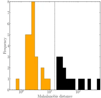
veloc-5 https://gaia.esac.esa.int/gost/ 100 101 102 Mahalanobis distance 0 1 2 3 4 5 6 7 8 F requency
Fig. B.1.Histogram of the Mahalanobis distance to the centre of the velocity distribution ( ˙ξ0
, ˙η0
, ˙ζ0
) of the 42 single sources of our sample. The vertical dashed line indicates the percentile p65used to select the
kinematic members (see Sect.2.3).
ity estimate (12.01±0.12 km s−1) is similar to a recent value from the literature (11.658 ± 0.006 km s−1,Soubiran et al. 2018).
2MASS J02232663+2244069. Our radial velocity measure-ment (12.60 ± 0.15 km s−1) is consistent with the one from the GaiaDR2 catalogue (12.1±0.6 km s−1). This source was listed as a high probability (99%) member of β Pic byMalo et al.(2013) based on a radial velocity and a proper motion which differ by 2 km s−1and 6 mas yr−1, respectively, from Gaia DR2. The dif-ferent data could explain why this source was discarded by our kinematic selection and the membership of this source has been revised with our data.
2MASS J03573393+2445106. We have three spectra for this source with radial velocity measures of 13.46 ± 0.18 km s−1 (2018-08-12), 13.44 ± 0.18 km s−1 (2018-08-14), and 15.30 ± 0.14 km s−1 (2019-11-30). This source is rotationally variable (0.86 days,Hartman et al. 2011) which could explain the vari-ations in the radial velocity that we measure. This source is a candidate of spectroscopic binary which requires more follow-up observations to confirm it. We also note thatCrundall et al. (2019) classified it as a field contaminant.
2MASS J05004928+1527006. This source was classified as a member by Schlieder et al. (2012) based on a predicted radial velocity of 13.70±2.03 km s−1. We measure a radial veloc-ity of 18.4 ± 0.3 km s−1, similar to what has been reported in the literature (White et al. 2007), and significantly different to the predicted value used in the previous membership analysis. Additionally, this source has been classified as a member of the Taurus-Auriga complex (Kraus et al. 2017), and therefore is a likely contaminant in β Pic.
2MASS J08475676-7854532. This source was classified as a candidate of β Pic based on a predicted radial velocity of 13.4± 1.5 km s−1(Malo et al. 2013). This value is significantly different from our measurement of 23.1±0.3 km s−1and with the literature (23.4 ± 0.3 km s−1 fromMalo et al. 2014a). Using Gaia, it has been proposed as a member of η Chamaeleontis (Cantat-Gaudin et al. 2018).