Comparison of tactile and chromatic confocal measurements of aspherical lenses for form metrology

HAL Id: hal-01069752

https://hal.archives-ouvertes.fr/hal-01069752

Submitted on 13 Oct 2017

HAL is a multi-disciplinary open access

archive for the deposit and dissemination of

sci-entific research documents, whether they are

pub-lished or not. The documents may come from

teaching and research institutions in France or

abroad, or from public or private research centers.

L’archive ouverte pluridisciplinaire HAL, est

destinée au dépôt et à la diffusion de documents

scientifiques de niveau recherche, publiés ou non,

émanant des établissements d’enseignement et de

recherche français ou étrangers, des laboratoires

publics ou privés.

Comparison of tactile and chromatic confocal

measurements of aspherical lenses for form metrology

Nadim El-Hayek, Hichem Nouira, Nabil Anwer, Mohamed Damak, Olivier

Gibaru

To cite this version:

Nadim El-Hayek, Hichem Nouira, Nabil Anwer, Mohamed Damak, Olivier Gibaru. Comparison of

tactile and chromatic confocal measurements of aspherical lenses for form metrology. International

Journal of Precision Engineering and Manufacturing, Korean Society of Precision Engineering„ 2014,

15 (5), pp.821-829. �10.1007/s12541-014-0405-y�. �hal-01069752�

Science Arts & Métiers (SAM)

is an open access repository that collects the work of Arts et Métiers ParisTech

researchers and makes it freely available over the web where possible.

This is an author-deposited version published in:

http://sam.ensam.eu

Handle ID: .

http://hdl.handle.net/10985/8649

To cite this version :

Nadim EL HAYEK, Hichem NOUIRA, Nabil ANWER, Mohamed DAMAK, Olivier GIBARU

-Comparison of tactile and chromatic confocal measurements of aspherical lenses for form

metrology - International Journal of Precision Engineering and Manufacturing - Vol. 15, n°5,

p.821-829 - 2014

Any correspondence concerning this service should be sent to the repository

Comparison of Tactile and Chromatic Confocal

Measurements of Aspherical Lenses for Form Metrology

El-Hayek Nadim

_{, Nouira Hichem}

_{, Anwer Nabil}

_{, Damak Mohamed}

_,

_{Gibaru Olivier}

1 Laboratoire Commun de Métrologie (LNE-CNAM), Laboratoire National de Métrologie et d’Essais (LNE), 1 Rue Gaston Boissier, 75015 Paris, France 2 Ecole Normale Supérieure de Cachan, University Research Laboratory in Automated Production, 61 avenue du Président Wilson, 94235 Cachan, France 3 GEOMNIA: 3D Metrology Engineering and Software Solutions, 165 Avenue de Bretagne, EuraTechnologies 59000 Lille, France 4 Arts et Métiers ParisTech, Laboratory of Information Sciences and Systems (LSIS), 8 Boulevard Louis XIV, 59046 Lille, France # Corresponding Author / E-mail: nadimhayek@gmail.com, TEL: +33-6-42-58-25-45, FAX: +33-1-40-43-37-37

KEYWORDS: Aspherical surface, Chromatic confocal probe, Form metrology, L-BFGS method, Profilometer, Tactile probe

Both contact and non-contact probes are often used in dimensional metrology applications, especially for roughness, form and surface profile measurements. To perform such kind of measurements with a nanometer level of accuracy, LNE (French National Metrology Institute (NMI)) has developed a high precision profilometer traceable to the SI meter definition. The architecture of the machine contains a short and stable metrology frame dissociated from the supporting frame. It perfectly respects Abbe principle. The metrology loop incorporates three Renishaw laser interferometers and is equipped either with a chromatic confocal probe or a tactile probe to achieve measurements at the nanometric level of uncertainty. The machine allows the in-situ calibration of the probes by means of a differential laser interferometer considered as a reference. In this paper, both the architecture and the operation of the LNE’s high precision profilometer are detailed. A brief comparison of the behavior of the chromatic confocal and tactile probes is presented. Optical and tactile scans of an aspherical surface are performed and the large number of data are processed using the L-BFGS (Limited memory-Broyden-Fletcher-Goldfarb-Shanno) algorithm. Fitting results are compared with respect to the evaluated residual errors which reflect the form defects of the surface.

1. Introduction

Europe has a leading role in high-end optical products,1 ultra-precise manufacturing and inspection systems.2-5 The core sectors being in photonics, lighting, biomedical technologies and optical systems, European shares of the global photonics market range from 25% to 45%.6 Discussions at the “4th High Level Expert Meeting of the Competence Centre for Ultra Precise Surface Manufacturing” on asphere metrology strongly emphasized the urgent needs of industry for more accurate form measurement and improved asphere standards traceable to the SI7 Measuring optical surfaces with a nanometric accuracy remains a real challenge in industry. Thus, in 2011, LNE has launched a three-year project entitled “optical and tactile metrology for absolute form characterization” as part of the European Metrology Research Programme8 (EMRP) with different NMI partners such as PTB, VSL, METAS, SMD, MKEH, IBSPE, TNO, CMI, EJPD, FhG, TU-IL and Xpress, with an aim to improve the measurement of high quality optical surfaces such as aspherical lenses. Current techniques

and processes allow for manufacturing aspherical surfaces with machining correction at the nanometer level.8 However, the accuracy accessible by absolute and traceable form metrology is limiting the manufacturing of modern optical elements, and has to be improved at the nanometer level of accuracy. In the field of ultra-precision 3D metrology, various small-volume coordinate measuring machines (CMMs) have been developed.9 These machines typically feature 3D measuring ranges less than 100×100×100 mm3, and usually apply the same set of fundamental principles. The main principle consists in achieving high positioning and measuring accuracy with perfect respect to Abbe principle.10 The instruments can be stylus-based11 or optical based.11,12 The traceability of these measuring apparatus are performed using laser interferometers which are traceable to the SI meter definition through a frequency calibration by comparison with an I2-stabilized primary He-Ne laser source.

In this context, the LNE has developed its own new high precision profilometer in collaboration with Digital-Surf Company. The architecture of the profilometer perfectly respects the Abbe principle.

The metrology loop is minimized as short as possible. The design of the profilometer allows both tactile and chromatic confocal probing. It is equipped with the MountainsMap® surface imaging and metrology software, which is useful for flat and step-height standards. However, this software is not adapted for freeform surfaces and does not include any fitting tools. For this purpose, different non-linear Least-Squares optimization techniques can be considered such as, Gauss-Newton methods, gradient descent methods, a mix of them (Levenberg-Marquardt13) or quasi-Newton methods. The quasi-Newton method called L-BFGS is proposed here for the form metrology of aspherical surfaces.14,15

This paper provides details about the architecture of the LNE high precision profilometer on which tactile and optical measurements have been performed. Since the probes represent fundamental elements of the metrology loop, their residual errors are briefly compared and discussed. The measurements are performed over a specific aspherical lens model defined by a conic and a polynomial. The orthogonal Least-Squares fitting of the data to the mathematical model is achieved by applying the L-BFGS optimization method and the residual errors representing the form deviations of the asphere are then compared. The experimental test results reveal that the tactile measurement is more accurate than the optical measurement.

2. The LNE High Precision Profilometer

The LNE's apparatus is a high precision profilometer capable of performing nanometric measurements. Three high precision guiding axes equipped with encoders insure three independent translational degrees of freedom, in x-, y- and z- directions (Fig. 1). A Zerodur table on which the measured object is posed travels along x- and y- directions and its movement is controlled by two independent Renishaw laser interferometers to a nanometric level of accuracy. The working range in the xy-plane is 50×50 mm². The fixture of the Zerodur table on the top side of the x-mechanical guiding system is carried-out via three ball with a diameter less than 10 mm, to insure an isostatic links. The probe and its supporting structure are mounted on the vertical guiding system in the z-direction along which the measurement is done (Figs. 1 and 2). The working range of the mechanical guiding system in z-direction is about 100 mm but then the practical working range strongly depends on the travel range of the probe used. A third Renishaw differential laser interferometer controls the movement in z with a nanometric level of accuracy and its use allows shortening the metrology loop. The metrology frame involves parts and components made of Invar which makes it less sensitive to thermal expansion and other environmental fluctuations. The thermal expansion coefficient of Invar is about 1µm/ m/oC. The thermal behavior of the metrology frame made of Invar with the dimensions of 200×200×200 mm3 is estimated by varying the surrounding temperature by 0.1°C. It generates a temperature change in the Invar structure of less than 0.01°C, especially when the variation of the environment temperature vary smoothly. For this case, the thermal expansion of the metrology frame is estimated to 2 nm which can be considered small. For Zerodur, the thermal expansion coefficient is about 0.05µm/m/°C and the dimensions of the table are 200×200×50 mm3. For the same temperature variation, the thermal expansion of the

table is even smaller and is estimated to 0.5 nm.

The mechanical guiding systems, the probe and the metrology frame are all supported by a structure made of massive granite. Any vertical expansion or deformation of the supporting frame does not influence the metrology frame since the vertical motion is controlled by the differential laser interferometer. The vertical thermal expansion of the granite structure induces an identical variation of the first and second laser beams of the differential interferometer and is therefore directly compensated. In a differential laser interferometer, only the variations of the distance between the external reference mirror and the external moving mirror are taken into account.

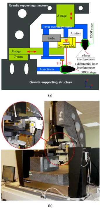
The high precision profilometer applies the dissociated metrology frame principle which means that the metrology frame is dissociated from the supporting frame. The metrology frame is fixed on the Fig. 1 The LNE's high precision profilometer. (a) architecture of the apparatus. (b) Picture of the apparatus

supporting frame using isostatic links (flexible blades) to avoid any transmission of eventual mechanical strain induced by the supporting frame. As a consequence, the metrology frame supports its own mass and only performs the function of measurement.16,17

The machine respects the Abbe principle in all directions11: the measuring probe's axis and the differential laser interferometer's beam are collinear during the measurement operation. However, during in-situ calibration, the Zerodur table remains fixed. This means that the reference mirror facing beam (1) in Fig. 2 becomes the moving reflector and the underside of the Zerodur table becomes the reference reflector. The touching element of the contact probe in the case of tactile measurement, or the focus point of the optical single point probe in the case of an optical measurement, are coplanar with the x- and y-laser interferometer beams. Since the x- and y- laser interferometers and the probe are all on the same metrology frame, any displacement of the frame induces a displacement of all these elements. The machine is configured to hold both tactile and optical single point scanning probes that can be calibrated in-situ. The Zerodur table is controlled by the three laser interferometers as mentioned above and shown in Fig. 1, so the reflecting elements and the interferometers should be well aligned. Each interferometer beam must be perpendicular to its target reflecting mirror and collinear with the respective direction of motion within the acceptable angle of 25 arc-seconds. A four quadrant photodiode fixed on the moving table is used for the alignment of each laser beam with the direction of motion. The laser beam must theoretically remain focused at the center of the photodiode over the entire travel range. The misalignment is measured and the average value found on this machine for x- and y- motions is about 50µrad per 50 mm range. The alignment error is estimated to 6.2510-8 mm and considered negligible. Since the x-, y- and z- motions are independent, the mirrors facing the laser interferometer beams should be orthogonal among themselves. The evaluation of orthogonality is performed using the LNE's coordinate

measuring machine (“CMM5”) which is accurate to 0.5µm over a working volume range of 0.5 m3. To guarantee such a volumetric uncertainty, the translation errors (two straightness and one positioning) for each mechanical guiding system, and the rotational errors (pitch, yaw and roll) are calibrated using a ball-bar (alternatively hole-bar) system. Many other instruments can be used for the calibration of CMM such as step gauges, gauge blocks, ball plates, the Zeiss CMM check artefact, hole plates, ball-ended bars, laser interferometers, tracking interferometers and tracer interferometers. The perpendicularity between each two axes is calibrated twice: first, using the ball-bar and then using an angle gauge block. For the perpendicularities between the x-, y- and z-axes, the uncertainty is estimated to 0.8”. More details about the calibration of CMM5 are widely presented in.18-21

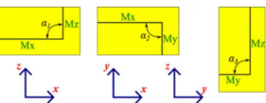
The perpendicularities between the different sides of the Zerodur table are measured by the CMM5 machine (Fig. 3). At least 10 points are measured on each side and the Least-Squares plane is fitted. The angles between normal directions to each of the planes are α1, α2 and α3 and are equal to 90°00'10"±0.8", 89°59'34"±0.8" and 89°59'18.1" ±0.8", respectively. These misalignments are tolerated since they are identified and compensated in the software.

The motion errors of the guiding elements induce inclination of the Zerodur table and must also be corrected in the software. These errors are characterized using the long-term extremely stable and accurate probe, Leica Nivel20 (0.001 mm/m). For the 50 mm working range of the apparatus, the motion induced inclination errors are below 1 nm.

The high precision profilometer is placed in the LNE's cleanroom where environmental conditions are optimal. The temperature is controlled to 20±0.3°C and humidity to 50±5%RH. The variation in temperature is very slow and smooth in the bandwidth ±0.3 which leads to a very low temperature variation in the parts of the machine.

The Newport anti-vibration system as shown in Fig. 1(b) attenuates all low-frequency vibrations generated by the surrounding environment. Furthermore, all the above system is mounted on a concrete anti low-frequency vibration massif that isolates it from the room floor.

The uncertainty budget established for the measurement according to the GUM,22 takes into consideration all of the aforementioned error sources such as: the error motions of the mechanical guide systems, the Abbe and cosine errors, the dynamics of the machine, the geometry of the Zerodur table, thermal drift and the tactile probe and laser interferometer errors. For the case of a flat artifact, uncertainty budget for a tactile measurement is established considering all sources of error. It results in an expanded uncertainty of 15+10-6 L (nm), using a coverage factor k of 2. This uncertainty is mainly affected by the performance and the behavior of the probe. The stated value is only valid for a flat artifact measured by tactile probing. When using chromatic confocal probing on aspherical artifacts, the uncertainty budget should be re-evaluated.

Fig. 2 Schematic of the metrology frame and illustration of all x-, y-and z- Abbe axes

3. Measurement Probes and Reference Interferometers

Classically, the measurement of aspherical surfaces is done using tactile probing also referred to as stylus profilometry.24 The probe's behavior highly contributes to the overall uncertainty of the measurement since it is involved in the metrology loop. The optical and tactile probes used are characterized and their uncertainty is estimated under similar environment conditions. Laser interferometers have also been previously calibrated.

3.1 Laser interferometers

Interferometry is the measure of interference between two signals. Within a laser interferometer, a laser source emits a beam towards an optical separator that divides it into two sub-beams. The first sub-beam travels towards a fixed reference reflector, the second one towards the reflector under displacement, in this case the Zerodur table's reflector. The beams are finally reflected back and they undergo interference. If no displacement takes place both signals are equal. On the contrary, if a displacement was measured, the second beam returns with a phase shift. The relationship between displacement and this phase change is given by the modified “Edlen” formula.24 The stability of the used Renishaw laser interferometers is less than 2 nm.

3.2 Chromatic confocal probe

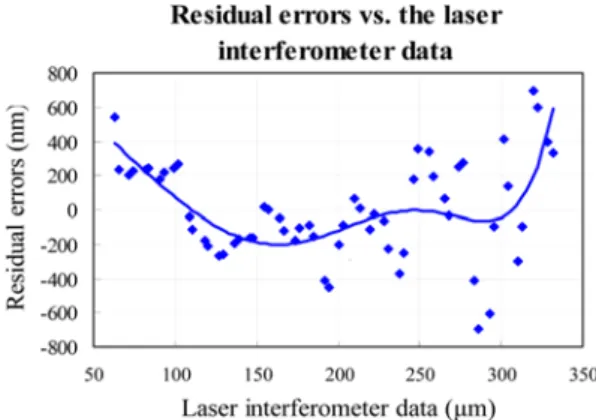
Chromatic confocal probes are introduced in ISO25178-602:2010 25 and used in many measurement applications, but most importantly, for surface profiling.26 They rely on a white light source LED whose spectral components are focused at different distances along the optical axis. The wavelength that is best focused on the surface being measured is the only wavelength that will be reflected back into the system. A mechanical filter adjusted for this principle guarantees this operation so the reflected light is collected and analyzed with a spectrometer. The working distance of the optical probe used is 350µm. Therefore, the in-situ calibration is performed over this travel range and repeated 60 times. A first in-situ calibration test is performed step-by-step over the travel range of 350µm by comparing the information given by the chromatic confocal probe to the information given by the differential laser interferometer. The conversion of the recorded confocal data to distance is achieved by a linear fit to cover the entire travel range. The obtained residual errors are within 800 nm (Fig. 4). This value is considered to be too large because the measurement precision is requested to be within few tens of nanometers. Based on this result and the works of Leach and Nouira et al,11,27,28 the behavior of the chromatic confocal probe seems to be complex and sensitive to many parameters, particularly, gap variations (residual errors and linearity), material, roughness, form, reflectivity and inclination of the workpiece, power of the light source, acquisition frequency and scanning speed.

It was concluded that it is complicated to develop a model that could consider the numerous error sources. Piecewise linear models are adopted here. They better reduce large residual errors over the entire travel range than polynomial models. Nevertheless, piecewise models does not take into account the effect of the angle deviation between the probe and the artifact, the form and reflectivity of the artifact, and all the other error sources related to the used aspherical artifact.

The in-situ calibration of the chromatic confocal probe is performed

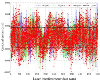
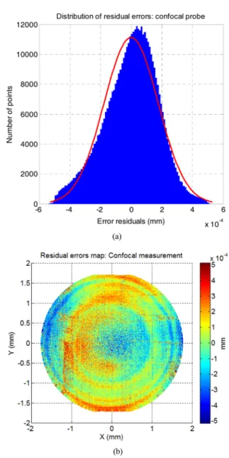
in dynamic operation mode. The conversion of the recorded confocal digital data to distance is achieved by applying a piecewise linear model with 2048 linear models. The residual errors that represent the difference between the confocal data and the laser interferometer data, with all corrections and compensations applied to the interferometric measurement, are obtained and illustrated in Fig. 5. The residual errors are about ±14 nm at the beginning of the working range and decrease to ±4 nm at the end of the working range, independently of the scanning speed ranging from 10 to 100µm/s.

The standard deviation of the residual errors is calculated and is equal to about ±2 nm (Fig. 5). Additionally, the obtained residuals present a Gaussian distribution (Fig. 6), which means, according to the Guide to the expression of Uncertainty in Measurement (GUM), that the standard uncertainty of the chromatic confocal probe can be estimated by dividing the bandwidth by the coverage factor of 3 for a confidence level of ~99%. This makes the standard uncertainty be equal to about ±0.6 nm when calibrated on a flat sample. However, the proposed correction strategy of the confocal data is sensitive to inclination. Additionally, the Fig. 4 Residual errors of confocal measurement versus laser interferometer data before applying any correction model

Fig. 5 In-situ calibration of the chromatic confocal probe over the entire working range of 350µm. Evolution of the residual errors versus the displacement measured by the z-differential laser interferometer for three values of speed: 10, 50 and 100µm/s (blue, green, red). Modeling of the data with a piecewise linear model of 2048 models giving a standard deviation of residual errors below 2 nm (black)

connection point between each two successive partial models can be erroneous and change from one type of artifact to the other, thus generating errors that can dramatically impact the mentioned value of 0.6 nm.

3.3 Tactile probe

The tactile probe's tip is a diamond stylus located on one end of a beam which pivots around its center point. On the other end, two coils measure the magnetic field induced by the pivoting amplitude. The primary and secondary coils are connected in an AC bridge circuit such that when the armature between them is centrally positioned no output is generated and the beam is in neutral position. Otherwise, when the beam is displaced, the magnetic field infers amplitude of displacement and the relative phase of the signal determines the direction. The probe is a stylus with a tip angle of 90°, a tip radius of 2µm and a static measuring force of 0.7 mN. It can be used in three different measurement ranges, a small range going from 0 to 100µm, a medium range going from 0 to 500µm and a large range going up to 1000 µm. The range selection depends on the depth to be measured on the surface. The probe is calibrated in-situ with a scanning speed of 10µm/s for the smallest working range [0 100] µm. A 9th_{-order polynomial model is} used to approximate the data and compensate for the bias errors. Fig. 7 shows that the residual errors fluctuate between ±20 nm. The standard deviation that results is about ±6 nm. Here again, the residual errors present a Gaussian distribution (Fig. 8) so the standard uncertainty can be calculated and is equal to ±2 nm.

4. Optical and Tactile Scanning of an Aspherical Surface

Due to their unmatched performance and to the advanced techniques that exist today for high precision manufacturing of complex optical components, aspherical and freeform optics have become a growing market. In metrological applications for example, aspherical lenses represent the ideal choice for light collimators in laser diodes. There are numerous manufacturing processes for aspherical lenses,29 but

collimators can be somehow complicated to manufacture as stated by Allen et al.5 In the present paper, a glass replication technology is used for the manufacturing of the tested aspherical lens.24 This technology offers the most cost effective solution for astigmatism, spherical aberration, coma and spherochromatism corrections. An asphere surface is classically defined by the model in Eq. (1).

Other definitions, such as the Forbes aspheres,30 exist and have been shown to be interesting. However, in this work, the measured asphere inherits the model of Eq.1 and is an axis-symmetric combination of a conic and a polynomial.

(1) Z f c( , ,κ α r;) cr 2 1+ 1–(1+κ)c2r2 --- α_2jr2j j=1 5

∑

Fig. 6 Distribution of the residual errors of the chromatic confocal probe's calibration

Fig. 7 In-situ calibration of the tactile probe over its smallest working range of 100µm at a fixed scanning speed of 10 µm/s; Evolution of the residual errors versus the displacement measured by the z-differential laser interferometer (blue) and the 9th order polynomial approximation of the data which gives a standard deviation for residual errors (y-std) less than 6 nm (red)

Fig. 8 Distribution of the residual errors of the tactile probe's calibration

where, r and Z are the coordinates of the aspherical surface. Real constants c, and are the curvature at the central point, the conic constant and the aspherical deformation constants, respectively. The surface has known model parameters and less than /20 Peak-to-Valley deviation surface errors at 633 nm wavelength, which is still a commonly adopted specification for surface quality (ISO10110-5,31 Fig. 9).

The measurements of the asphere take place in the LNE's cleanroom. About 500,000 points are recorded in the form of 3.5×3.5 mm² XY-grids and the table's motion is constantly controlled by the laser interferometers (Fig. 2). The optical probe's total measurement time is about half of the tactile probe's total measurement time (7.5 hours) since no contact needs to be established for the optical measurement.

5. Fitting Aspherical Data for Comparison

Form errors are calculated and surface form is characterized in this section. Fitting is the process of aligning together two geometrical entities by optimizing transformation parameters. For aspherical fitting, the L-BFGS algorithm is proposed.15

The L-BFGS method is an iterative quasi-Newton method used to solve unconstrained non linear optimization problems. This method is particularly interesting for problems with many variables and large data. The main advantage of this method is that it does not have to solve any linear equations and that the inverse Hessian matrix does not need to be exactly calculated, but only approximated. L-BFGS updates the inverse of the Hessian matrix by using information from the last m iterations, and each time, the new approximation replaces the oldest one in the queue. In a recent study, L-BFGS has been shown to be faster than traditional optimization methods for the fitting of B-Spline curves. Zheng et al.32 propose a simultaneous optimization of location parameters and control points which runs faster than other methods based on a sequential. For an objective function f with gradient g and hessian H, having x as the vector of variables, the algorithm goes as follows:

a) Initialization:

Make an initial guess for the solution, x0, and the Hessian H0 and choose a number m of iterations for the Hessian update. Then set two real values β' and β such that 0 < β' < ½ and β' < β < 1.

b) Iterations:

(2) where, dk= -Hkgk is the line search direction and αk is the step length in that direction which satisfies the Wolfe conditions:

(3) c) Updating:

The Hessian update is written as follows:

(4) Where ∆h depends on the change X = αkdk and the change G in the gradient.

For every Hessian update, L-BFGS stores the X and G vectors. All the way through the iterations of step b, H is updated as in Eq. (5). The parameter m defines a storage limit in L-BFGS, so that after m iterations, the oldest change h, is replaced by the newest. Since large volumes of data and many variables are dealt with in this paper limited storage is required.

(5)

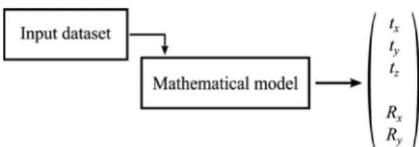
The fitting of aspherical surfaces is the process of aligning data points to their mathematical model. It requires optimizing for five out of six transformation parameters (Fig. 10): three translations in x-, y-and z- directions y-and two rotations about the x- y-and y- axes. Rotation about the z-axis is redundant because the asphere is axis-symmetric about z. The objective function to minimize is given by Eq. (6).

(6) N being the number of points in the dataset; Rθ,γ is the combined rotation matrix due to angles about x and about y.

This objective function is the minimization of the sum of squared distances between the data and the model. The works of Ahn33 on the fitting of parametric curves and surfaces and some parallel works done by the authors on the fitting of aspherical surfaces have shown that orthogonal distance minimization is more accurate than vertical distance minimization.

It has been also proven in parallel work done by El-Hayek et al. that this algorithm is as robust as the classical Levenberg-Marquardt

x_{k 1+} =x_k+a_kd_k f x( _k+α_kd_k) f x≤ ( ) β′α_k + _kg_kTd_k gT(x_k+α_kd_k)d_k≥βd_kTd_k H_{k 1+} =H_k+∆h X G H( , , _k) H₁=H₀+∆h X( ₀, ,G₀H₀) H₂=H₀+∆h X( ₀, ,G₀H₀)+∆h X( ₁, ,G₁H₁) … H_m=H₀+∆h X( ₀, ,G₀H₀)+∆h X( ₁, ,G₁H₁)+…+∆h X( _{m 1–},G_{m 1–},H_{m 1–} ) min (p_i–R_{θ γ,} P_i+T)2 i=0 N

∑

Fig. 9 Aspherical surface schematic and the coordinate variables

algorithm. Nevertheless, it offers the possibility to perform simultaneous calculations of the footpoints (projections of data points onto the model) and the transformation parameters. As compared to the Iterative Closest Point (ICP)34 algorithm used in registration/alignment applications but which can also be modified to be used in fitting applications, L-BFGS is more robust to the point-set's initial alignment with respect to the model. ICP fails if the initial position of the dataset is far from the optimal position. Furthermore, ICP uses discrete data, model points or a mesh of these, and that makes it the least complex among all algorithms. However, it requires that the number of points (or triangles in case of a mesh) be equivalent because each point must have an associated counterpart. In addition, the discrete model should be dense enough to match the sought level of precision.

6. Results and Analysis

The results of the L-BFGS fitting of the aspheric lens on both the tactile and the optical measured datasets are detailed and compared here. The residual errors of each of the fitting processes translate the form defects. It is shown that these form defects are directly affected by the measurement uncertainty of each of the measurement probes and by some additional error sources (the machine's guiding elements, the table motion, the geometry of the measured surface, its reflectivity, etc…). Experiments have shown that an optimal value of the storage limitation parameter m falls in the range of 7 to 20 iterations. 11 iterations are considered here. Similar initial positions of the dataset with respect to the model and identical initial guesses are verified. For an equal number of points in both datasets, the results of the L-BFGS fit are reported in Table 1 and the residual errors distributions and error maps are plotted on both Figs. 11 and 12. Table 1 shows that the evaluation of form defects with the tactile measurement returns more accurate results than the ones obtained from the optical measurement. The Root Mean Square (RMS) residual is 44 nm in the case of the tactile measurement and 177 nm RMS in the case of the optical measurement. Fig. 11 illustrates the distribution of the residual errors of the optical dataset fitting. The residuals do not follow a normal distribution for the mean value and standard deviation they have. The signed mean is equal to -0.25 nm and the standard deviation is about 177 nm (negative skewness equal to -0.27).

Fig. 12 points out the distribution of the residual errors of the tactile dataset fitting. The distribution is again not a normal distribution with the mean and standard deviation given. In this case, the signed mean is equal to 0.0378 nm and the standard deviation is about 44 nm (positive skewness value of 0.52). Since the chromatic confocal probe is in-situ calibrated on a single point on the aspherical lens, the geometry of the asphere, its inclination, its reflectivity and its roughness influence the uncertainty of the measurement. This clearly explains the observed difference in the output residual errors between the two measurements. In fact, the piecewise linear models ignore all these error sources.

7. Conclusion

The comparison of optical and tactile measurements of an asphere

using the LNE high precision profilometer is done based on form characterization and residual errors analysis. The design and the metrology performance of the developed apparatus are detailed and analyzed. Tactile and chromatic confocal probing reveal nanometric residual errors when calibrated on a flat standard. However, when used on aspherical artefacts, their behaviors are affected by other sources of error and the measurements are consequently biased. With disregard to the approximation of measurement residual errors and the strategies used to do so, tactile probing is more accurate than confocal probing. Table 1 Surface form characterization based on L-BFGS fitting with orthogonal distance minimization; (meas.: measurement, PV: Peak-to-Valley)

Absolute Mean (nm) RMS (nm) PV (nm) Optical meas. 142 177 1058

Tactile meas. 33 44 818

Fig. 11 Optical measurement residual errors for a clear aperture of r = 1.75 mm. (a) Histogram distribution of the residual errors (blue) and theoretical normal distribution fit (red) around the average and for a span from -3σ to 3σ; (b) residual errors map

As a future work, authors would like to investigate more about the measurement data approximation.

ACKNOWLEDGEMENT

This work is part of EMRP Joint Research Project-IND10 “Optical and tactile metrology for absolute form characterization” project. The EMRP is jointly funded by the EMRP participating countries within EURAMET and the European Union.

REFERENCES

1. Beckstette, K. F., “Trends in Asphere and Freeform Optics,” Proc. of Optonet Workshop, 2008.

2. Dumas, P R., Fleig, J., Forbes, G. W., Golini, D., Kordonski, W. I., and et al., “Flexible Polishing and Metrology Solutions for Free-Form Optics,” http://aspe.net/publications/Winter_2004/PAPERS/ 3METRO/1372.PDF (Accessed 16 APR 2014)

3. Wanders, G., “Advanced Techniques in Freeform Manufacturing,” Proc. of Optonet Workshop, 2006.

4. Karow, H. H., “Fabrication Methods for Precision Optics,” Wiley, Chap. 5, pp. 334-578, 1993.

5. Yi, A. Y., Huang, C., Klocke, F., Brecher, C., Pongs, G., and et al., “Development of a Compression Molding Process for Three-Dimensional Tailored Free-Form Glass Optics,” Applied Optics, Vol. 45, No. 25, pp. 6511-6518, 2006.

6. Photonics 21, “Lighting the Way Ahead,” 2010.

7. European Association of National Metrology Institutes, “EMRP Call 2010-Industry & Environment,” http://www.euramet.org/index. php?id=emrp_call_2010#c10140.html (Accessed 16 APR 2014) 8. Lee, W. B., Cheung, C. F., Chiu, W. M., and Leung, T. P., “An

Investigation Of Residual Form Error Compensation in the Ultra-Precision Machining of Aspheric Surfaces,” Journal of Materials Processing Technology, Vol. 99, No. 1, pp. 129-134, 2000. 9. Nouira, H., Bergmans, R., Küng, A., Piree, H., Henselmans, R., and

Spaan, H.A.M., “Ultra-High Precision CMMs as well as Tactile and Optical Single Scanning Probes Evaluation in Dimensional Metrology,” Proc. of CAFMET, 2014.

10. Abbé, E., “Meßapparate Für Physiker,” Zeitschrift Für Instrumentenkunde, Vol. 10, No. pp. 446-447, 1890.

11. Leach, R., “Optical Measurement of Surface Topography,” Springer, pp. 71-106, 2011.

12. Whitehouse, D. J., “Surfaces and Their Measurement,” Taylor & Francis, 2002.

13. Moré, J. J., “The Levenberg-Marquardt Algorithm: Implementation and Theory,” Numerical Analysis, pp.105-116, 1978.

14. Liu, D. C. and Nocedal, J., “On the Limited Memory BFGS Method for Large Scale Optimization,” Mathematical Programming, Vol. 45, No. 1-3, pp. 503-528, 1989.

15. Nocedal, J., “Updating Quasi-Newton Matrices with Limited Storage,” Mathematics of Computation, Vol. 35, No. 151, pp. 773-782, 1980. 16. Vissiere, A., Nouira, H., Damak, M., Gibaru, O., and David, J., “A

Newly Conceived Cylinder Measuring Machine and Methods that Eliminate the Spindle Errors,” Measurement Science and Technology, Vol. 23, No. 9, Paper No. 094015, 2012.

17. Vissiere, A., Nouira, H., Damak, M., Gibaru, O., and David, J., “Concept and Architecture of a New Apparatus for Cylindrical Form Measurement with a Nanometric Level of Accuracy,” Measurement Science and Technology, Vol. 23, No. 9, Paper No. 094014, 2012. 18. Zelený, V. and Stejskal, V., “The Most Recent Ways of CMM

Calibration,” http://home.mit.bme.hu/~kollar/IMEKO-procfiles-for-Fig. 12 Tactile measurement residual errors for a clear aperture of r =

1.75 mm. (a) Histogram distribution of the residual errors (blue) and theoretical normal distribution fit (red) around the average and for a span from -3σ to 3σ; (b) residual errors map

web/congresses/WC-16th-Wien-2000/Papers/Topic%2008/Zeleny. PDF (Accessed 25 MAR 2014)

19. Thalmann, R., “A New High Precision Length Measuring Machine,” Proc. of 8th International Congress of Metrology, 1997.

20. Flack, D., “Good Practice Guide No. 42-CMM Verification,” National Physical Laboratory, No. 2, 2011.

21. ISO 103606, “Geometrical Product Specifications (GPS) -Acceptance and Reverification Tests for Coordinate Measuring Machines (CMM) - Part 6: Estimation of Errors in Computing Gaussian associated Features,” 2001.

22. JCGM, “Evaluation of Measurement Data - Guide to the Expression of Uncertainty in Measurement,” 2008.

23. Lee, C. O., Park, K., Park, B. C., and Lee, Y. W., “An Algorithm for Stylus Instruments to Measure Aspheric Surfaces,” Measurement Science and Technology, Vol. 16, No. 5, pp. 1215, 2005.

24. Stone, J., Phillips, S. D., and Mandolfo, G. A., “Corrections for Wavelength Variations in Precision Interferometric Displacement Measurements,” Journal of Research of the National Institute of Standards and Technology, Vol. 101, pp. 671-674, 1996.

25. BS EN ISO 25178-602, “Geometrical Product Specifications (GPS). Surface Texture. Areal Nominal Characteristics of Non-Contact (Confocal Chromatic Probe) Instruments,” 2010.

26. Vaissiere, D., “Métrologie tridimensionnelle des états de surface par microscopie confocale à champ étendu,” Ph.D. Thesis, Sciences et Technologeis Industrielles, University of Strasbourg, France, 2003. 27. Nouira, H., El-Hayek, N., Yuan, X., Anwer, N., and Salgado, J.,

“Metrological Characterization of Optical Confocal Sensors Measurements,” Proc. of 14th International Conference on Metrology and Properties of Engineering Surfaces, 2013.

28. Nouira, H., El-Hayek, N., Yuan, X., and Anwer, N., “Characterization of the Main Error Sources of Chromatic Confocal Probes for Dimensional Measurement,” Measurement Science and Technology, Vol. 25, No. 4, Paper No. 044011, 2014.

29. Fang, F., Zhang, X., Weckenmann, A., Zhang, G., and Evans, C., “Manufacturing and Measurement of Freeform Optics,” CIRP Annals-Manufacturing Technology, Vol. 62, No. 2, pp. 823-846, 2013. 30. Forbes, G. W., “Shape Specification for Axially Symmetric Optical

Surfaces,” Optics Express, Vol. 15, No. 8, pp. 5218-5226, 2007. 31. ISO/DIS 10110-5, “Optics and Photonics - Preparation of Drawings

for Optical Elements and Systems - Part 5: Surface Form Tolerances,” 2007.

32. Zheng, W., Bo, P., Liu, Y., and Wang, W., “Fast B-Spline Curve Fitting by L-BFGS,” Computer Aided Geometric Design, Vol. 29, No. 7, pp. 448-462, 2012.

33. Ahn, S. J., “Least Squares Orthogonal Distance Fitting of Curves and Surfaces in Space,” Document ID : LNCS 3151, Springer, 2004. 34. Pomerleau, F., Colas, F., Siegwart, R., and Magnenat, S., “Comparing

ICP Variants on Real-World Data Sets,” Autonomous Robots, Vol. 34, No. 3, pp. 133-148, 2013.