HAL Id: hal-02901284
https://hal.sorbonne-universite.fr/hal-02901284
Submitted on 17 Jul 2020
HAL is a multi-disciplinary open access
archive for the deposit and dissemination of sci-entific research documents, whether they are pub-lished or not. The documents may come from teaching and research institutions in France or abroad, or from public or private research centers.
L’archive ouverte pluridisciplinaire HAL, est destinée au dépôt et à la diffusion de documents scientifiques de niveau recherche, publiés ou non, émanant des établissements d’enseignement et de recherche français ou étrangers, des laboratoires publics ou privés.
Claire Jacquet, Isabelle Gounand, Florian Altermatt
To cite this version:
Claire Jacquet, Isabelle Gounand, Florian Altermatt. How pulse disturbances shape size-abundance pyramids. Ecology Letters, Wiley, 2020, 23 (6), pp.1014-1023. �10.1111/ele.13508�. �hal-02901284�
How pulse disturbances shape size-abundance pyramids
Claire Jacquet1,2*, Isabelle Gounand1,2,3, Florian Altermatt1,2
1 Department of Aquatic Ecology, Swiss Federal Institute of Aquatic Science and Technology,
Eawag, Dübendorf, Switzerland
2 Department of Evolutionary Biology and Environmental Studies, University of Zurich, Zürich,
Switzerland
3 Sorbonne Université, CNRS, UPEC, CNRS, IRD, INRA, Institut d’écologie et des sciences de
l’environnement, IEES,, Paris, France
* corresponding author: phone: +41 58 765 6726, fax: +41 58 765 5802
Authors’ e-mail addresses: [email protected], [email protected],
Statement of authorship: CJ and FA designed research, CJ conducted the experimental
research, CJ and IG designed the theoretical research and IG did the mathematics and simulations to produce the theoretical figures. CJ wrote the first draft of the manuscript and all authors
critically contributed to the edition of the paper. 1
Keywords: perturbations, extreme events, metabolic theory, body-size, community
size-structure, size spectrum, protist communities, disturbance frequency, disturbance intensity.
Running title: How pulse disturbances shape size-abundance pyramids. Type of article: Letter.
Abstract: 144 words. Main text: 4750 words. References: 67.
The manuscript contains 6 Figures and Supporting Information. 2
Abstract
3
Ecological pyramids represent the distribution of abundance and biomass of living organisms 4
across body-sizes. Our understanding of their expected shape relies on the assumption of invariant 5
steady-state conditions. However, most of the world’s ecosystems experience disturbances that 6
keep them far from such a steady state. Here, using the allometric scaling between population 7
growth rate and body-size, we predict the response of size-abundance pyramids within a trophic 8
guild to any combination of disturbance frequency and intensity affecting all species in a similar 9
way. We show that disturbances narrow the base of size-abundance pyramids, lower their height 10
and decrease total community biomass in a nonlinear way. An experimental test using microbial 11
communities demonstrates that the model captures well the effect of disturbances on empirical 12
pyramids. Overall, we demonstrate both theoretically and experimentally how disturbances that are 13
not size-selective can nonetheless have disproportionate impacts on large species. 14
16
INTRODUCTION
17
Ecological pyramids, which represent the distribution of abundance and biomass of 18
organisms across body-sizes or trophic levels, reveal one of the most striking regularities among 19
communities (Elton 1927; Lindeman 1942; Trebilco et al. 2013). Several types of pyramids have 20
been reported in ecological research, as well as distinct underlying mechanisms to explain their 21
shape. For example, trophic pyramids describe the distribution of abundance or biomass along 22
discrete trophic levels (Fig. 1a). The inefficiency in energy transfer from resources to consumers 23
as well as strong self-regulation within trophic levels provide the main explanation for their shape 24
(Lindeman 1942; Barbier & Loreau 2019). Alternatively, size-abundance pyramids (Fig. 1b,c), also 25
known as the pyramid of numbers (Elton 1927), the Damuth law (Damuth 1981), or the abundance 26
size spectrum (Sprules & Barth 2016), describe the distribution of abundance across body-sizes 27
and can be studied both within and across trophic guilds (Elton 1927; Trebilco et al. 2013). The 28
energetic equivalence rule, along with the metabolic theory of ecology, provide theoretical 29
expectations regarding the shape of such size-abundance pyramids: in a community where all 30
individuals feed on a common resource (i.e. within a trophic group), population abundance should 31
be proportional to 𝑀"#.%&, where M is body-size, and biomass should be proportional to 𝑀#.(& 32
(Damuth 1981; Brown et al. 2004; White et al. 2007). 33
As with most concepts in ecology, these relationships correspond to theoretical baselines 34
that are predicted under steady-state conditions, which are rarely met in nature (DeAngelis & 35
Waterhouse 1987; Hastings 2004, 2010). Most natural ecosystems and communities are exposed 36
to a wide range of environmental fluctuations and disturbances, ranging from harvesting to extreme 37
weather events. Furthermore, many of these disturbances are expected to increase in frequency and 38
intensity in the context of global change, as illustrated by recent large scale wildfires, floods or 39
hurricanes (Coumou & Rahmstorf 2012; Hughes et al. 2017; Harris et al. 2018). Such disturbances 40
increase population mortality and could trigger even faster changes in community structure and 41
dynamics than gradual changes in average conditions (Jentsch et al. 2009; Wernberg et al. 2013; 42
Woodward et al. 2016). 43
Despite the extensive literature on disturbance ecology (Sousa 1984; Yodzis 1988; Petraitis 44
et al. 1989; Fox 2013; Dantas et al. 2016; Thom & Seidl 2016), the effects of disturbances on 45
community structure and biomass distribution remain poorly understood (Donohue et al. 2016). 46
On the one hand, ecologists have often focused on the consequences of environmental disturbances 47
on species richness (Huston 1979; Haddad et al. 2008; Bongers et al. 2009) and the coexistence of 48
competing species (Violle et al. 2010; Miller et al. 2011; Fox 2013), rather than on body-size and 49
biomass distribution (but see Woodward et al. (2016)). As such, the specific identity of species 50
resistant (or not) to disturbances has received ample attention, with various definitions of 51
disturbance-resistant species groups (Sousa 1980, 1984; Lavorel et al. 1997). These studies have 52
pointed out key demographic traits, notably population growth rate and carrying capacity, that 53
determine species’ capacities to persist in a disturbed environment (McGill et al. 2006; Haddad et 54
al. 2008; Enquist et al. 2015; Woodward et al. 2016). On the other hand, the metabolic theory of 55
ecology uses the scaling of metabolic rate with body-size to predict a set of structural and functional 56
characteristics across biological scales (Brown et al. 2004). At the community level, it 57
demonstrates how size-abundance pyramids emerge from the scaling of population growth rate and 58
abundance with body-size (Trebilco et al. 2013). Surprisingly, a formal integration of the theory 59
on disturbances with the metabolic theory of ecology is still lacking, but would allow ecologists to 60
generalize and predict the effect of environmental disturbances on the shape of size-abundance 61
pyramids. 62
Here, we integrate these two disconnected fields by developing a size-based model for 63
population persistence, assuming that the scaling of population growth rate with body-size is the 64
leading mechanism determining the response of size-abundance pyramids to disturbances. We 65
predict the shape of size-abundance pyramids within a trophic guild in response to repeated pulse 66
disturbances of varying frequency and intensity affecting all species in a similar way, regardless of 67
their size. Such disturbances represent a wide range of environmental pressures that increase 68
species mortality, such as floods, wildfires, or hurricanes. They differ from the disturbance studies 69
developed in fishery sciences, that specifically addressed the effect of a press, size-selective 70
disturbance (i.e. fishing) on the abundance size spectrum (Jennings et al. 2002; Shin et al. 2005; 71
Petchey & Belgrano 2010; Sprules & Barth 2016). We then experimentally test the predicted 72
responses of size-abundance pyramids and standing biomass to disturbances, using microbial 73
communities composed of aquatic species with body-sizes and populations densities varying over 74
several orders of magnitudes. We finally discuss the general implications of our findings for the 75
structure and functioning of communities exposed to environmental disturbances. 76
77
MATERIALS AND METHODS
78
A model for size-abundance pyramids exposed to disturbances
79
We build a mechanistic model to predict how disturbance frequency and intensity modulate 80
the shape of size-abundance pyramids and community total biomass. We describe the dynamics of 81
population abundance N with a logistic model: 82 )* )+ = 𝑟𝑁 /1 − * 23 (1) 83
where r is population growth rate and K is population carrying capacity. We model a disturbance 84
regime, corresponding to a recurrent abundance reduction, of intensity I (fraction of abundance) 85
and frequency f or period T=1/f (time between two disturbances, Fig. 2a). We can demonstrate that 86
a population persists in a disturbed environment only if its growth rate balances the long-term effect 87
of the disturbance regime (adapted from Harvey et al. 2016), that is: 88
𝑟 > − 56(8"9); (2)
89
From equation (2), we can predict the set of disturbance regimes a population can sustain 90
according to its growth rate (Fig. 2b), as well as the minimum generation time (1/r) needed to 91
maintain a viable population (Fig. S1). We then use the allometric relationship between population 92
growth rate r and average body-size M, that is 𝑟 = 𝑐 × 𝑀> with a = –¼ (Brown et al. 2004; 93
Savage et al. 2004) and c a positive constant, to derive the following size-specific criterion for 94
population persistence under a disturbance regime: 95
𝑀 ≤ /56 (8" 9);×@ 3"A (3) 96
Equation (3) indicates that a species can persist in a disturbed environment only if its average body-97
size is below a certain value. Note that this analytical criterion is applicable to any biological and 98
temporal scale. Indeed, the disturbance frequency and population growth rate are expressed with 99
the same time unit and can range from hours (e.g. fast-growing microbial organisms) to years (e.g. 100
slow-growing organisms such as large mammals). To investigate the effect of disturbances on the 101
shape of size-abundance pyramids, we derive the mean abundance at dynamical equilibrium 𝑁B of 102
a population under a given disturbance regime (i.e. averaged over a time period, see Appendix 1 103
for detailed steps), that is: 104
𝑁B = 𝐾 /DE(8"9);×F + 13 (4)
105
where 𝐾 corresponds to the carrying capacity of the population, which also scales with body-size 106
on a logarithmic scale (Brown & Gillooly 2003; Brown et al. 2004): 𝑙𝑛(𝐾) = 𝑎2ln(𝑀) + 𝑏2, 107
where aK and bK are normalizing constants. We use this allometric relationship to express mean
108
abundance as a function of mean population body-size and finally obtain: 109
𝑙𝑛(𝑁B) = 𝑎2ln(𝑀) + 𝑏2+ 𝑙𝑛 /;NOP QR(S)T UP DE(8"9) + 13 (5) 110
The formula is valid when the expression in parentheses in the right-hand term is positive, which 111
corresponds to the persistence criteria given in equations (2) and (3). We express population 112
biomass, B, as the product of mean abundance at dynamical equilibrium, 𝑁B, and the average 113
individual body-size in the population, 𝑀, that is 𝐵 = 𝑁B𝑀. 114
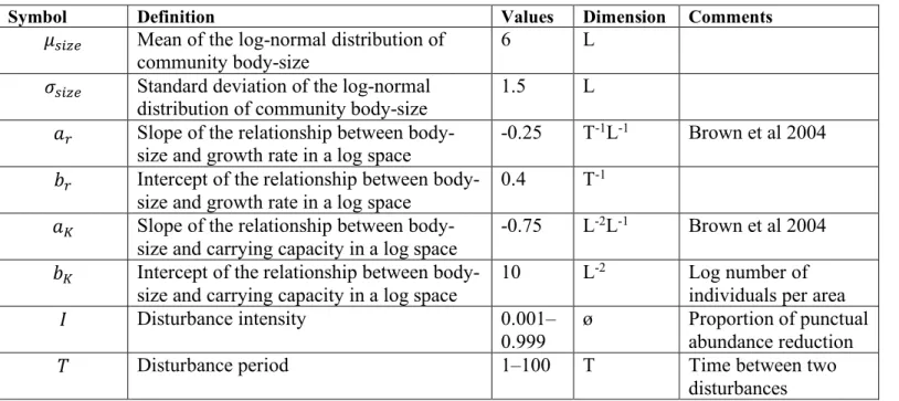
We extend this approach to multispecies assemblages composed of potentially hundreds of 115
co-occurring species with different body-sizes (see detailed method in Appendix 2 and Table S1 116
for parameter values). We assume that all species’ populations follow a logistic growth and are 117
constrained by intraspecific competition only (an assumption relaxed in Appendix 3). From 118
equation (3) and (5), we expect that disturbances will decrease the maximum size observed in the 119
community as well as total biomass. We use this analytical approach to explore how community 120
size-structure, a more tractable representation of abundance distribution across size-classes 121
compared to pyramids (Fig. 1b), and total community biomass will respond to a whole landscape 122
of disturbance frequencies and intensities (Fig. 3). 123
124
Disturbance experiment on microbial communities
125
We conducted an experiment in aquatic microcosms inoculated with 13 protist species and 126
a set of common freshwater bacteria as a food resource. The protist species cover a wide range of 127
body-sizes (from 10–103 µm) and densities (10–105 individuals/ml, Giometto et al. 2013). General
128
lab procedures follow the protocols described in Altermatt et al. (2015), and build upon previous 129
work on pulse disturbance effects on diversity (Altermatt et al. 2011; Harvey et al. 2016) and 130
invasion dynamics (Mächler & Altermatt 2012). Detailed microcosm description and set-up are 131
presented in Appendix 4. In short, we performed a factorial experiment in which we varied 132
disturbance frequency and intensity, resulting in a total of twenty different disturbance regimes. 133
Disturbance was achieved by boiling a subsampled fraction of the well-mixed community in a 134
microwave so that all species experience the same level of density reduction. All protists were 135
killed by the microwaving process. We let the medium cool down before putting it back into the 136
microcosm. We disturbed microcosms at five intensities: 10, 30, 50, 70 and 90 % and at four 137
frequencies: f= 0.08, 0.11, 0.16 and 0.33, corresponding to a disturbance every 12, 9, 6 and 3 days, 138
respectively. The experiment lasted for 21 days, or about 10–50 generations depending on species. 139
Each disturbance regime was replicated six times. To control for the intrinsic variability of 140
community size-structure, we cultured eight undisturbed microcosms under the same conditions. 141
We sampled 0.2 ml of each microcosm daily to quantify individual body-sizes (i.e. cell area in 142
µm2), protist abundances (individuals/µl) and total community biomass (i.e. total bioarea in
143
µm2/µl) using a standardized video procedure (Altermatt et al. 2015; Pennekamp et al. 2017). We
144
binned the observed individuals into twelve size-classes ranging from 0 to 1.6´105 µm2 in order to
145
get statistically comparable community size-structures. Mean protist abundance and its standard 146
deviation in each size-class were calculated over 21 time points and 6 replicates (total of 126 147
observations) for each treatment and over 21 time points and 8 replicates (total of 168 observations) 148
for the control communities. We performed Welch two sample t-tests of mean comparison 149
(treatment versus control) to determine which disturbance regime had a significant effect on 150
community size-structure and total community biomass (Table S2). 151
152
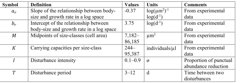
Model parameterization
We parameterized the model using the experimental data in order to test the capacity of the model 154
to predict the effect of a given disturbance regime on the size-structure of real communities. The 155
model required the following input parameters: the carrying capacities of each size-class as well as 156
the slope and the intercept of the allometric relationship between growth rate and body-size. We 157
took the average abundances of the undisturbed communities (8 controls) to the estimate carrying 158
capacities in each size-class. We fitted a logistic growth model to the recovery dynamics of each 159
size-class after one disturbance (I = 90%) to obtain growth rate estimations. Specifically, we used 160
the data from the treatment {I=90%, f =0.08} (i.e. highest intensity, lowest frequency) to estimate 161
the parameters of a logistic growth model over 12 time points using the function nls() of the stats 162
package in R (R Core Team 2019). We determined the relationship between growth rate and body-163
size in our experimental communities using the 13 time-series (covering 6 size-classes) that 164
displayed a logistic growth. We obtained the following allometric relationship: 𝑙𝑛(𝑟) = 165
−0.37 × ln(𝑀) + 3.75 (p-value = 0.005, R2 = 0.47). Using this parameterization, we produced
166
theoretical predictions on the size-abundance pyramids expected in the experimental disturbance 167
regimes. We then quantitively compared these predictions with the size-abundance pyramids 168
observed in the experimental communities. We performed ordinary least-squares regressions to 169
characterize the relationship between observed and predicted log-transformed mean abundances 170
among size-classes for all the disturbance regimes. 171 172 RESULTS 173 Model predictions 174
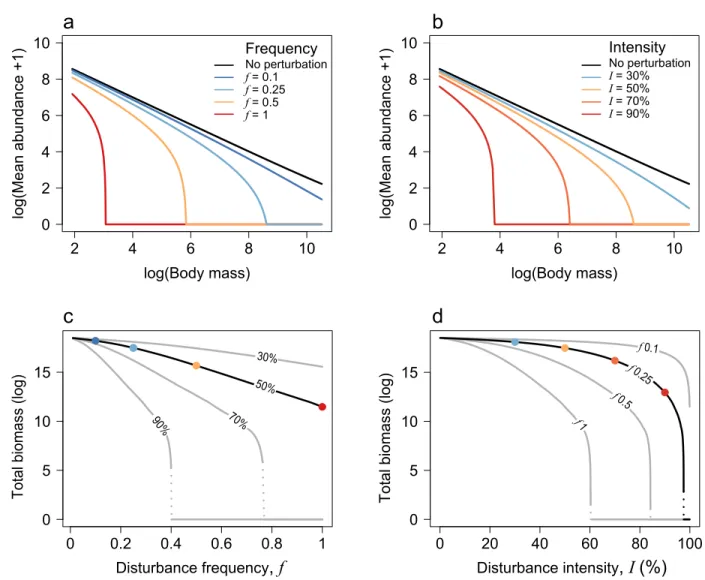
We first explore the effects of increasing disturbance frequency (Fig. 3a, c). Infrequent 175
disturbances do not strongly affect community size-structure and only decrease the mean 176
abundance of the largest size-classes (Fig. 3a, f = 0.1 in dark blue). Maximum body-size gradually 177
decreases as disturbance frequency increases, corresponding to the extinction of large, slow-178
growing species (Fig. 3a, f = 0.25 in light blue). Disturbance frequency also affects the community 179
size-structure through its effect on mean abundance. For frequent disturbance events, the mean 180
abundance of all size-class decreases (Fig. 3a, f = 0.5 and 1 in orange and red respectively). The 181
effect of disturbance frequency on community-size structure have direct consequences for 182
community-level properties: we indeed observe an approximately linear decrease in total 183
community biomass (log) along a gradient of disturbance frequency, followed by an abrupt collapse 184
of the community for extreme disturbance regimes (Fig. 3c). 185
We then investigate the effect of increasing disturbance intensity (Fig. 3b, d). Similarly, 186
low intensity disturbances marginally affect community size-structure (Fig. 3c, I = 30% in blue) 187
and increasing disturbance intensity decreases maximum body-size and population mean 188
abundance. (Fig. 3b). Interestingly, the effect of disturbance intensity on community total biomass 189
is clearly nonlinear (Fig. 3d). Low to intermediate disturbance intensities do not affect total biomass 190
when disturbance frequency is low (e.g. f = 0.1 or 0.25 in Fig. 3d). However, strong intensities 191
affect all population abundances and trigger a sharp decrease in total biomass, culminating in a 192
crash of the system (e.g. {I > 90%, f = 0.25} in Fig 3d). 193
194
Experimental results
195
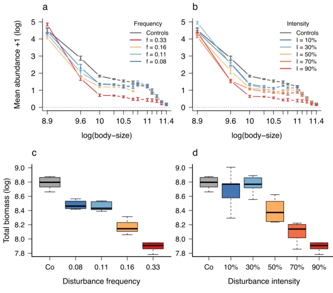
We experimentally investigated the effect of disturbance frequency and intensity on the 196
size-structure of microbial communities. For a fixed intensity (set to I = 90% in Fig. 4a, see Fig. 197
S2 for other intensities), infrequent disturbances (i.e. f = 0.08 and f = 0.11) had a significant 198
negative impact only on the mean abundance of intermediate size-classes (between exp(9.6) and 199
exp(10.5) µm2, Welch two sample t-tests: t ³ 2.6, p-values £ 0.02, Table S2). When disturbance
frequency increased to f = 0.16, the mean abundance of the smallest size-class also decreased (t = 201
3.6, p-value = 0.01, Table S2). Finally, at even more frequent disturbances (f = 0.33), all size-202
classes were negatively impacted, except the smallest one (Fig 5a and Table S3). Overall, 203
increasing disturbance frequency led to an abundance depletion at intermediate sizes compared to 204
undisturbed control communities. 205
Similarly, for a fixed frequency (set to f = 0.33 in Fig. 4b, see Fig. S3 for other frequencies), 206
a low disturbance intensity I = 10 % (Fig. 4b) only affected intermediate size-classes (between 207
exp(10) and exp(10.5) µm2, t ³ 4.5, p-values £ 0.001, Table S2). Disturbance intensities I = 30%
208
and 50% had a negative effect on the mean abundance of larger size-classes (between exp(10) and 209
exp(11) µm2, t ³ 2.8, p-values £ 0.03, Table S2). Finally, intensities I = 70% and I = 90% had an
210
impact on all size-classes, except the smallest size-class that were not negatively impacted by 211
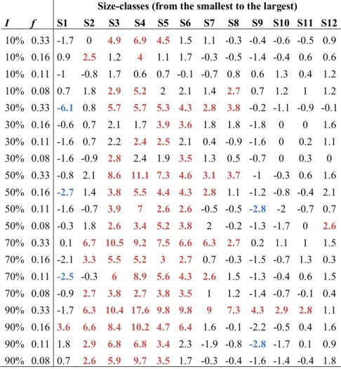
change in disturbance intensity (Fig. 4b, Table S2). Interestingly, the following disturbance 212
regimes had a positive effect of on the mean abundance of the smallest size-class: {I = 30%, f = 213
0.33}, t = -6.1, p-value < 0.001, (Fig. 4b), as well as {I = 50%, f = 0.16} and {I = 70%, f = 0.11} 214
(Table S2, Fig. S2 and S3). 215
At the community-level, total biomass gradually decreased with disturbance frequency as 216
expected by theory (Fig. 4c). All frequencies had a significant negative effect on total biomass 217
compared to controls (t ³ 8, p-value < 0.001, Fig 4c). Disturbance intensities I = 10% and 30% had 218
no significant effects on total community biomass (I10%: t = 0.75, p-value = 0.48, I30%: t = 0.5,
p-219
value = 0.63), while total biomass strongly decreased for intensities above I = 50% (I50%: t = 6.1,
220
p-value < 0.001, I70%: t = 12.7, p-value < 0.001, I90%: t = 14.2, p-value < 0.001, Fig. 4d).
221 222
Observed versus predicted effect of disturbances on size-abundance pyramids
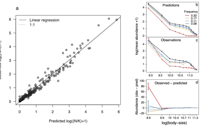
We then compared our experimental results with the predictions of the model parameterized 224
for our freshwater microbial communities (Figure 5). The model predicted well the observed mean 225
abundances relative to carrying capacity for all the disturbance regimes in most of the size-classes. 226
The slope of the linear regression between observed and predicted log mean abundances, including 227
all size-classes in all disturbance regimes (240 points), was very close to the 1:1 line, which 228
indicates a very good fit (Figure 5a, linear regression: y = -0.012 + 1.01x, R2 = 0.96, p-value <
229
0.001). Additionally, the intercept of the linear regression was not significantly different from zero 230
(t = 0.95, p-value = 0.34). We illustrate in Figure 5b-d the similarities as well as the differences 231
between the predicted and observed community size-structures for varying disturbance frequencies 232
with a disturbance intensity fixed to I = 90% (other disturbance regimes are shown in Figs. S4-S5). 233
Overall, the predicted community structures were very similar to the observed ones. The model, 234
however, often underestimated the mean abundance in the smallest size-class (Figure 5d). 235
Furthermore, as mentioned in the previous section, some disturbance regimes had a positive effect 236
of on the mean abundance of the smallest size-class, which cannot, by construction, be predicted 237
by our model. We discuss below how this pattern can be explained by a disruption of biotic 238
interactions following a disturbance and present further analyses using a predator-prey model to 239
support this possible explanation (Fig. 6c, Appendix 3). 240
241
DISCUSSION
242
Most theories in community ecology have been developed under the assumption of steady-243
state conditions (Hastings 2010). Yet, most of the world’s ecosystems – specifically ≥75% of 244
land/freshwater and 50% of marine systems – have been altered by human activities and are facing 245
disturbances that put them clearly outside of such a steady state (IPBES 2018). Thus, to meet the 246
societal demand for an ecological science able to predict how ecosystems will respond to global 247
change (Petchey et al. 2015; Urban et al. 2016), this assumption needs to be relaxed. The challenge 248
is to develop models that make quantitative predictions regarding the impact of fluctuating 249
environmental conditions on the structural and functional characteristics of biological systems. 250
251
Consequences of the growth-size relationship for communities exposed to disturbances
252
Here, we provide a robust and simple approach for predicting the size-structure of 253
communities exposed to any combination of disturbance frequency and intensity affecting all 254
species in a similar way, regardless of their body-size. We combine theory on disturbances with 255
the metabolic theory of ecology and assume that the scaling of population growth rate with body-256
size is the leading mechanism determining the response of size-abundance pyramids to 257
disturbances. The model makes an important advance over the steady-state predictions of the 258
metabolic theory of ecology as it links quantitatively the shape of a size-abundance pyramid to the 259
disturbance regime experienced by the community (Fig. 6a–b). Overall, increasing disturbance 260
frequency or intensity narrows the bases of size-abundance pyramids and lowers their height. This 261
corresponds to the extinction of the largest species and a general reduction of population mean 262
abundances in all size-classes. Hence, we demonstrate that disturbances that are not size-selective 263
and do not target large species have nonetheless a higher impact on large species than on smaller 264
ones. 265
The model is applicable across all biological and temporal scales as population growth rate 266
and disturbance frequency are expressed with the same time units. Equation (2) can also apply to 267
populations that do not show a scaling relationship between growth rate and body-size and predicts 268
which disturbance regimes a species can sustain, or not, based on its generation time (Figs. 2 and 269
S1). Importantly, our results are not specific to repeated pulse disturbances but also hold for press 270
disturbances, which will affect the shape of size-abundance pyramids in an equivalent way (see 271
Appendix 1 for a mathematical demonstration). 272
Our model offers a new perspective on community responses to disturbances by exploring 273
the effect of repeated pulse disturbances of varying frequency and intensity on community size 274
structure. The majority of theoretical studies on community stability have focused on local stability, 275
which examine community’s response to small pulse disturbances around one single equilibrium 276
(Donohue et al. 2016), reflecting the great interest for the so-called diversity-stability debate (May 277
1972; McCann 2000; Allesina & Tang 2012; Jacquet et al. 2016). Our approach goes beyond local 278
stability measures at the vicinity of one single attractor and is applicable to any combination of 279
disturbance frequency or intensity. It predicts which species, based on its growth rate, can persist 280
or not and how the abundances of the remaining species will be affected by a whole gradient of 281
disturbances. 282
Note that the model depends on a number of technical assumptions. First, we restricted our 283
theoretical approach to disturbance regimes where pulse disturbances are applied at fixed intervals 284
with a fixed intensity. This choice, though relatively simplistic, allowed us to mirror the disturbance 285
regimes applied to the experimental communities. To generalize, we also performed simulations 286
where we added stochasticity in the frequency and intensity of the disturbance regime to test the 287
sensitivity of the theoretical results to variability in the periodicity and intensity of disturbances 288
(Appendix 2). Our results were qualitatively robust to the addition of noise around average values 289
of disturbance frequency and intensity, which simply increased the negative effect of one given 290
disturbance regime on the largest size-classes (Fig. S6). Second, we consider that the allometric 291
parameters of the relationships between population growth rate, carrying capacity and body-size 292
are the same for all species (i.e. same slopes and intercepts). We therefore performed sensitivity 293
analyses of Equation (5) and demonstrate that our results are robust to variation in these allometric 294
parameters (Appendix 2, Fig. S7-8). 295
296
Experimental test of the theory
297
The disturbance experiment on microbial communities showed some similarities but also 298
some departures from the theoretical predictions (Figure 5b-d). As expected from the analytical 299
model, total community biomass gradually decreased with disturbance frequency and in a more 300
nonlinear way with disturbance intensity (Fig. 4c–d, and Fig. 3c–d for the theoretical predictions). 301
Interestingly, it was the intermediate and not the largest size-classes that were the most sensitive 302
to disturbances in the microbial community. We provide below two possible explanations for this 303
observation. Most likely, the abundances of the largest size-class might be already too low, and 304
therefore too close to the methodologically-defined detection threshold, in the control communities 305
to observe a significant effect of the disturbances of these size-classes. Second, this might be 306
explained by the duration of the experiment (21 days), which was not long enough to capture the 307
extinction of the largest species. We estimated the time to reach the dynamical equilibrium in the 308
experiment with the model parameterized with experimental data (see Table S3). The model 309
predicted that equilibrium is reached by the end of the experiment (21 days) for the size-classes 310
considered in all disturbance regimes but the strongest. With the highest frequency and intensity 311
{I=90%; f=0.33} the equilibrium is reached by the three smallest size-classes (in 12, 18, and 21 312
days respectively). 313
Additionally, some combinations of disturbance frequency and intensity had a positive 314
effect on the smallest size-class of microbes compared to controls, which corresponded to the main 315
departure from the theoretical predictions (Figure 4a-b and Figure 5d). This could be explained by 316
a disruption of biotic interactions (predation or competition) following a disturbance, allowing the 317
remaining small species to grow in higher densities in the absence of other species (Cox & Ricklefs 318
1977; Ritchie & Johnson 2009; Bolnick et al. 2010). Such “interaction-release” mechanism could 319
not be captured by our model of co-occurring species. We discuss below how interspecific 320
interactions, such as competition, predation or parasitism, could modulate the shape of size-321
abundance pyramids exposed to disturbances. 322
323
Extending the model to communities of interacting species
324
To observe an “interaction-release” effect that will widen the pyramid’s base, two 325
conditions are required (but not sufficient): (i) the existence of a significant mismatch between the 326
growth rates of the two interacting species, leading to differential response to disturbances, and (ii) 327
the species with the slowest growth rate has a negative effect on the other species (i.e. predator, 328
competitor or parasite). The latter condition seems unlikely for parasitism. For competitive 329
interactions, a “competition-release” effect can potentially increase the abundance of small, fast-330
growing species that will recover faster from a disturbance event compared to larger competitors 331
(e.g. Xi et al. (2019)). Finally, the existence of a “predation-release” effect is very likely as 332
predators are generally larger than their prey and have slower growth rates (Brose et al. 2006, 2016; 333
Barnes et al. 2010). In an additional analysis, we performed simulations using a predator-prey 334
model to explore in which conditions a “predation-release” effect could increase the abundance of 335
small prey species (see Appendix 3 for detailed methods). We found that small to intermediate 336
disturbance regimes can increase average prey abundance through a “predation-release” effect, 337
which should generate size-abundance pyramids with a wider base (Fig. 6c). This effect vanishes 338
above some disturbance thresholds, where prey species are also negatively impacted by 339
disturbances (Fig. 6c and Figs. S9-S11). 340
Our model cannot capture cascading effects triggered by complex interactions networks in 341
its current form. A promising future direction is the extension of the model to multitrophic 342
communities, which will allow further explorations of the potential of interspecific interactions to 343
modulate the impact of disturbances on size-abundance pyramids and community biomass. Indeed, 344
it is likely that predator species will also be impacted indirectly through a bottom-up transmission 345
of the disturbances (i.e. decrease in prey availability). 346
347
Additional mechanisms shaping size-abundance pyramids exposed to disturbances
348
Here, we propose a systematic approach, based on the metabolic theory of ecology, to 349
predict the response of size-abundance pyramids to persistent disturbances. Our results are specific 350
to a class of persistent disturbances (i.e. pulse or press) that affect the abundance of all species in 351
a similar way, regardless of their specific body-size or growth rate. We also assume that the leading 352
mechanism that determines the response of size-abundance pyramids to this type of disturbances 353
is the allometric relationship between species growth rate and body-size. However, additional 354
mechanisms can generate size-dependent abundances or size-dependent responses to disturbances 355
in real world ecosystems. First, species sensitivity to disturbances that are not size-selective can be 356
nonetheless unequal among size classes, with particular size-classes being more resistant to a given 357
disturbance intensity. For example, strong windstorms or droughts generally cause greater 358
mortality among larger or taller trees (Woods 2004; Hurst et al. 2011; Bennett et al. 2015). Second, 359
from a spatial perspective, size-specific mobility and immigration-extinction dynamics could 360
largely affect the relationship between species recovery dynamics and their size (McCann et al. 361
2005; Jacquet et al. 2017). It would be interesting to extend our approach to metacommunities, 362
where the depletion of large species in a disturbed habitat patch could be balanced by immigration 363
from undisturbed neighboring patches (Pawar 2015). 364
Finally, some disturbances can be size-selective, as illustrated by studies on abundance size 365
spectra that specifically addressed the effect of a press, size-selective disturbance, often reflecting 366
disturbances expected under commercial fishing (Shin et al. 2005; Sprules & Barth 2016). Our 367
model can easily be refined to more specific cases, in which disturbances have unequal effects on 368
species, by adding size-specific disturbance intensities to the model. The abundance size spectra 369
of harvested fish communities are generally characterized by steeper slopes than unfished 370
communities, and are used as a size-based indicator of fisheries exploitation (Shin et al. 2005; 371
Petchey & Belgrano 2010; Sprules & Barth 2016). We demonstrate that size-abundance pyramids 372
are also predictably affected by more general pulse disturbances that are not size-selective such as 373
floods or wildfires. Hence, when compared to a reference state, size-abundance pyramids provide 374
information on the level of disturbances an ecosystem is facing and could be used as “universal 375
indicators of ecological status”, as advocated in Petchey & Belgrano (2010). 376
377
Conclusion
378
Our findings have direct implications regarding the effects of disturbances on ecosystem 379
functioning. Indeed, the model makes predictions on total biomass and demographic traits 380
correlated to productivity rate and energy flows, which are among the most relevant metrics to 381
quantify ecosystem functioning (Oliver et al. 2015; Schramski et al. 2015; Brose et al. 2016; 382
Barnes et al. 2018). In the current context of global change, we demonstrate that the expected 383
increase in disturbance frequency and intensity should accelerate the extinction of the largest 384
species, leading to an increasing proportion of communities dominated by small, fast-growing 385
species and lower levels of standing biomass. Importantly, the effect of increasing disturbance 386
regimes will be nonlinear and abrupt changes in community structure and functioning are expected 387
once a disturbance threshold affecting the equilibrium abundances of smaller species is reached. 388
389
DATA AVAILABILITY STATEMENT
390
The data supporting the experimental results as well as a Rmarkdown document, which explains 391
in detail the theoretical approach and produces the figures, are archived in the Dryad Digital 392 Repository: https://doi.org/10.5061/dryad.95x69p8g7. 393 394 ACKNOWLEDGEMENT 395
We thank Sereina Gut, Samuel Hürlemann and Silvana Käser for help during the laboratory work 396
and Chelsea J. Little for comments on the manuscript. We also thank Jean François Arnoldi, 397
Samraat Pawar and two anonymous reviewers for their helpful comments on previous versions of 398
the manuscript. Funding is from the Swiss National Science Foundation Grants No 399
PP00P3_179089, the University of Zurich Research Priority Program “URPP Global Change and 400
Biodiversity” (both to F.A.) and the University of Zurich Forschungskredit (to C.J. and I.G.). 401
402
REFERENCES
403
Allesina, S. & Tang, S. (2012). Stability criteria for complex ecosystems. Nature, 483, 205–208. 404
Altermatt, F., Fronhofer, E.A., Garnier, A., Giometto, A., Hammes, F., Klecka, J., et al. (2015). 405
Big answers from small worlds: a user’s guide for protist microcosms as a model system in 406
ecology and evolution. Methods Ecol. Evol., 6, 218–231. 407
Altermatt, F., Schreiber, S. & Holyoak, M. (2011). Interactive effects of disturbance and dispersal 408
directionality on species richness and composition in metacommunities. Ecology, 92, 859– 409
870. 410
Barbier, M. & Loreau, M. (2019). Pyramids and cascades: a synthesis of food chain functioning 411
and stability. Ecol. Lett., 22, 405–419. 412
Barnes, A.D., Jochum, M., Lefcheck, J.S., Eisenhauer, N., Scherber, C., O’Connor, M.I., et al. 413
(2018). Energy Flux: The Link between Multitrophic Biodiversity and Ecosystem 414
Functioning. Trends Ecol. Evol., 33, 186–197. 415
Barnes, C., Maxwell, D., Reuman, D.C. & Jennings, S. (2010). Global patterns in predator — 416
prey size relationships reveal size dependency of trophic transfer efficiency. Ecology, 91, 417
222–232. 418
Bennett, A.C., McDowell, N.G., Allen, C.D. & Anderson-Teixeira, K.J. (2015). Larger trees 419
suffer most during drought in forests worldwide. Nat. Plants, 1, 15139. 420
Bolnick, D.I., Ingram, T., Stutz, W.E., Snowberg, L.K., Lau, O.L. & Paull, J.S. (2010). 421
Ecological release from interspecific competition leads to decoupled changes in population 422
and individual niche width. Proc. R. Soc. B, 277, 1789–1797. 423
Bongers, F., Poorter, L., Hawthorne, W.D. & Sheil, D. (2009). The intermediate disturbance 424
hypothesis applies to tropical forests, but disturbance contributes little to tree diversity. Ecol. 425
Lett., 12, 798–805. 426
Brose, U., Blanchard, J.L., Eklöf, A., Galiana, N., Hartvig, M., R. Hirt, M., et al. (2016). 427
Predicting the consequences of species loss using size-structured biodiversity approaches. 428
Biol. Rev., 49, n/a-n/a. 429
Brose, U., Jonsson, T. & Berlow, E.L. (2006). Consumer-resource body size relationships in 430
natural food webs. Ecology, 87, 2411–2417. 431
Brown, J.H. & Gillooly, J.F. (2003). Ecological food webs : High-quality data facilitate 432
theoretical unification. Proc. Natl. Acad. Sci., 100, 1467–1468. 433
Brown, J.H., Gillooly, J.F., Allen, A.P. & Savage, V.M. (2004). Toward a metabolic theory of 434
ecology. Ecology, 85, 1771–1789. 435
Coumou, D. & Rahmstorf, S. (2012). A decade of weather extremes. Nat. Clim. Chang., 2, 491– 436
496. 437
Cox, G.W. & Ricklefs, R.E. (1977). Species Diversity and Ecological Release in Caribbean Land 438
Bird Faunas. Oikos, 28, 113. 439
Damuth, J. (1981). Population density and body size in mammals. Nature, 290, 699–700. 440
Dantas, V. de L., Hirota, M., Oliveira, R.S. & Pausas, J.G. (2016). Disturbance maintains 441
alternative biome states. Ecol. Lett., 19, 12–19. 442
DeAngelis, D.L. & Waterhouse, J.C. (1987). Equilibrium and Nonequilibrium Concepts in 443
Ecological Models. Ecol. Monogr., 57, 1–21. 444
Donohue, I., Hillebrand, H., Montoya, J.M., Petchey, O.L., Pimm, S.L., Fowler, M.S., et al. 445
(2016). Navigating the complexity of ecological stability. Ecol. Lett., 19, 1172–1185. 446
Elton, C. (1927). Animal Ecology. Macmillan. 447
Enquist, B.J., Norberg, J., Bonser, S.P., Violle, C., Webb, C.T., Henderson, A., et al. (2015). 448
Scaling from Traits to Ecosystems: Developing a General Trait Driver Theory via 449
Integrating Trait-Based and Metabolic Scaling Theories. Adv. Ecol. Res., 52, 249–318. 450
Fox, J.W. (2013). The intermediate disturbance hypothesis should be abandoned. Trends Ecol. 451
Evol., 28, 86–92. 452
Giometto, A., Altermatt, F., Carrara, F., Maritan, A. & Rinaldo, A. (2013). Scaling body size 453
fluctuations. Proc. Natl. Acad. Sci., 110, 4646–4650. 454
Haddad, N.M., Holyoak, M., Mata, T.M., Davies, K.F., Melbourne, B.A. & Preston, K. (2008). 455
Species’ traits predict the effects of disturbance and productivity on diversity. Ecol. Lett., 456
11, 348–356. 457
Harris, R.M.B., Beaumont, L.J., Vance, T.R., Tozer, C.R., Remenyi, T.A., Perkins-Kirkpatrick, 458
S.E., et al. (2018). Biological responses to the press and pulse of climate trends and extreme 459
events. Nat. Clim. Chang., 8, 579–587. 460
Harvey, E., Gounand, I., Ganesanandamoorthy, P. & Altermatt, F. (2016). Spatially cascading 461
effect of perturbations in experimental meta-ecosystems. Proc. R. Soc. B, 283, 20161496. 462
Hastings, A. (2004). Transients: the key to long-term ecological understanding? Trends Ecol. 463
Evol., 19, 39–45. 464
Hastings, A. (2010). Timescales, dynamics, and ecological understanding. Ecology, 91, 3471– 465
3480. 466
Hughes, T.P., Kerry, J.T., Álvarez-Noriega, M., Álvarez-Romero, J.G., Anderson, K.D., Baird, 467
A.H., et al. (2017). Global warming and recurrent mass bleaching of corals. Nature, 543, 468
373–377. 469
Hurst, J.M., Allen, R.B., Coomes, D.A. & Duncan, R.P. (2011). Size-Specific Tree Mortality 470
Varies with Neighbourhood Crowding and Disturbance in a Montane Nothofagus Forest. 471
PLoS One, 6, e26670. 472
Huston, M. (1979). A General Hypothesis of Species Diversity. Am. Nat., 113, 81–101. 473
IPBES. (2018). Summary for policymakers of the global assessment report on biodiversity and 474
ecosystem services of the Intergovernmental Science-Policy Platform on Biodiversity and 475
Ecosystem Services. 476
Jacquet, C., Moritz, C., Morissette, L., Legagneux, P., Massol, F., Archambault, P., et al. (2016). 477
No complexity–stability relationship in empirical ecosystems. Nat. Commun., 7, 12573. 478
Jacquet, C., Mouillot, D., Kulbicki, M. & Gravel, D. (2017). Extensions of Island Biogeography 479
Theory predict the scaling of functional trait composition with habitat area and isolation. 480
Ecol. Lett., 20, 135–146. 481
Jennings, S., Warr, K.J. & Mackinson, S. (2002). Use of size-based production and stable isotope 482
analyses to predict trophic transfer efficiencies and predator-prey body mass ratios in food 483
webs. Mar. Ecol. Prog. Ser., 240, 11–20. 484
Jentsch, A., Kreyling, J., Boettcher-Treschkow, J. & Beierkuhnlein, C. (2009). Beyond gradual 485
warming: Extreme weather events alter flower phenology of European grassland and heath 486
species. Glob. Chang. Biol., 15, 837–849. 487
Lavorel, S., McIntyre, S., Landsberg, J. & Forbes, T.D.A. (1997). Plant functional classifications: 488
from general groups to specific groups based on response to disturbance. Trends Ecol. Evol., 489
12, 474–478. 490
Lindeman, R. (1942). The trophic-dynamic aspect of ecology. Ecology, 23, 399–417. 491
Mächler, E. & Altermatt, F. (2012). Interaction of Species Traits and Environmental Disturbance 492
Predicts Invasion Success of Aquatic Microorganisms. PLoS One, 7. 493
May, R.M. (1972). Will a large complex system be stable? Nature, 238, 413–4. 494
McCann, K.S. (2000). The diversity-stability debate. Nature, 405, 228–233. 495
McCann, K.S., Rasmussen, J.B. & Umbanhowar, J. (2005). The dynamics of spatially coupled 496
food webs. Ecol. Lett., 8, 513–23. 497
McGill, B., Enquist, B.J., Weiher, E. & Westoby, M. (2006). Rebuilding community ecology 498
from functional traits. Trends Ecol. Evol., 21, 178–85. 499
Miller, A.D., Roxburgh, S.H. & Shea, K. (2011). How frequency and intensity shape diversity-500
disturbance relationships. Proc. Natl. Acad. Sci., 108, 5643–5648. 501
Oliver, T.H., Heard, M.S., Isaac, N.J.B., Roy, D.B., Procter, D., Eigenbrod, F., et al. (2015). 502
Biodiversity and Resilience of Ecosystem Functions. Trends Ecol. Evol., 30, 673–684. 503
Pawar, S. (2015). The Role of Body Size Variation in Community Assembly. Trait. Ecol. - From 504
Struct. to Funct. 1st edn. Elsevier Ltd. 505
Pennekamp, F., Griffiths, J.I., Fronhofer, E.A., Garnier, A., Seymour, M., Altermatt, F., et al. 506
(2017). Dynamic species classification of microorganisms across time, abiotic and biotic 507
environments—A sliding window approach. PLoS One, 12, e0176682. 508
Petchey, O.L. & Belgrano, A. (2010). Body-size distributions and size-spectra: universal 509
indicators of ecological status? Biol. Lett., 6, 434–437. 510
Petchey, O.L., Pontarp, M., Massie, T.M., Kéfi, S., Ozgul, A., Weilenmann, M., et al. (2015). 511
The ecological forecast horizon, and examples of its uses and determinants. Ecol. Lett., 18, 512
597–611. 513
Petraitis, P.S., Latham, R.E. & Niesenbaum, R.A. (1989). The Maintenance of Species Diversity 514
by Disturbance. Q. Rev. Biol., 64, 393–418. 515
Ritchie, E.G. & Johnson, C.N. (2009). Predator interactions, mesopredator release and 516
biodiversity conservation. Ecol. Lett., 12, 982–998. 517
Savage, V.M., Gillooly, J.F., Brown, J.H. & Charnov, E.L. (2004). Effects of body size and 518
temperature on population growth. Am. Nat., 163, 429–41. 519
Schramski, J.R., Dell, A.I., Grady, J.M., Sibly, R.M. & Brown, J.H. (2015). Metabolic theory 520
predicts whole-ecosystem properties. Proc. Natl. Acad. Sci., 112, 2617–2622. 521
Shin, Y.-J., Rochet, M.-J., Jennings, S., Field, J.G. & Gislason, H. (2005). Using size-based 522
indicators to evaluate the ecosystem effects of fishing. ICES J. Mar. Sci., 62, 384–396. 523
Sousa, W.P. (1980). The responses of a community to disturbance: the importance of 524
successional age and species’ life histories. Oecologia, 45, 72–81. 525
Sousa, W.P. (1984). The Role of Disturbance in Natural Communities. Annu. Rev. Ecol. Syst., 15, 526
353–391. 527
Sprules, W.G. & Barth, L.E. (2016). Surfing the biomass size spectrum: Some remarks on 528
history, theory, and application. Can. J. Fish. Aquat. Sci., 73, 477–495. 529
Thom, D. & Seidl, R. (2016). Natural disturbance impacts on ecosystem services and biodiversity 530
in temperate and boreal forests. Biol. Rev. Camb. Philos. Soc., 91, 760–781. 531
Trebilco, R., Baum, J.K., Salomon, A.K. & Dulvy, N.K. (2013). Ecosystem ecology: size-based 532
constraints on the pyramids of life. Trends Ecol. Evol., 28, 423–431. 533
Urban, M.C., Bocedi, G., Hendry, A.P., Mihoub, J.-B., Peer, G., Singer, A., et al. (2016). 534
Improving the forecast for biodiversity under climate change. Science (80-. )., 353, 535
aad8466–aad8466. 536
Violle, C., Pu, Z. & Jiang, L. (2010). Experimental demonstration of the importance of 537
competition under disturbance. Proc. Natl. Acad. Sci., 107, 12925–12929. 538
Wernberg, T., Smale, D.A., Tuya, F., Thomsen, M.S., Langlois, T.J., De Bettignies, T., et al. 539
(2013). An extreme climatic event alters marine ecosystem structure in a global biodiversity 540
hotspot. Nat. Clim. Chang., 3, 78–82. 541
White, E.P., Ernest, S.K.M., Kerkhoff, A.J. & Environnement, E.T. (2007). Relationships 542
between body size and abundance in ecology. Trends Ecol. Evol., 22, 323–30. 543
Woods, K.D. (2004). Intermediate disturbance in a late-successional hemlock-northern hardwood 544
forest. J. Ecol., 92, 464–476. 545
Woodward, G., Bonada, N., Brown, L.E., Death, R.G., Durance, I., Gray, C., et al. (2016). The 546
effects of climatic fluctuations and extreme events on running water ecosystems. Philos. 547
Trans. R. Soc., 371, 20150274. 548
Xi, W., Peet, R.K., Lee, M.T. & Urban, D.L. (2019). Hurricane disturbances, tree diversity, and 549
succession in North Carolina Piedmont forests, USA. J. For. Res., 30, 219–231. 550
Yodzis, P. (1988). The Indeterminacy of Ecological Interactions as Perceived Through 551
Perturbation Experiments. Ecology, 69, 508–515. 552
554 555
Figure 1: A trophic pyramid (a) describes the distribution of biomass along discrete trophic levels,
556
and assumes that all species within a trophic level have the same functional traits. The community 557
size-structure (b) and the size-abundance pyramid (c) are equivalent size-centric representations of 558
ecological communities and are the focus of this study. They describe the distribution of abundance 559
across body-sizes and can be studied both within and across trophic levels. b) the community size-560
structure depicts log(body-size) on the x-axis and log(abundance) on the y-axis, while c) the size-561
abundance pyramid shows log(abundance) on the x-axis and log(body-size) on the y-axis. Note 562
that the area A is the same in both panels. We use the community size-structure representation 563
throughout the paper as it facilitates comparisons between theory and experimental data, but see 564
Fig. 6 for a synthesis of our findings using the pyramid representation. 565
567
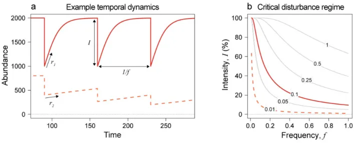
Figure 2: Population dynamics and persistence according to disturbance regime. a) Temporal
568
dynamics of two species experiencing the same disturbance regime. Species 1 has a smaller body-569
size and therefore a higher growth rate than species 2. A population can persist only if its growth 570
rate balances the long-term effect of the disturbance regime. We derive in equation (4) the mean 571
abundance at dynamical equilibrium (i.e. temporal mean) of the persisting species experiencing 572
varying disturbance regimes. b) Isoclines of the persistence criterion in the disturbance regime 573
landscape according to population growth rate (numbers): on and above the line, the population of 574
a given growth rate goes extinct. Lines with the same color code as in panel (a) correspond to the 575
same growth rate. 576
578
579
Figure 3: Effects of disturbance frequency and intensity on community size-structure and average
580
total biomass at dynamical steady state. Analytical results derived from Equation (5). a) Effect of 581
disturbance frequency (disturbance intensity is fixed to 50% abundance reduction), and b) 582
disturbance intensity (disturbance frequency is fixed to 0.25) on community size-structure. c) 583
Effect of disturbance frequency and d) intensity on average total biomass (in log), for different 584
intensities (c) and frequencies (d), respectively. Points on the black lines in (c) and (d) show the 585
disturbance regimes corresponding to community size-structures of the respective colors displayed 586
in panels (a) and (b). 587 0 5 10 15 0 0.2 0.4 0.6 0.8 1 0 5 10 15 0 20 40 60 80 100
a
b
c
d
No perturbation I = 30% I = 50% I = 70% I = 90% Intensity No perturbation f = 0.1 f = 0.25 f = 0.5 f = 1 FrequencyDisturbance frequency, f Disturbance intensity, I (%)
Total biomass (log) Total biomass (log)
30% 50% 70% 90% f 0.1 f 0.25 f 0.5 f 1 2 4 6 8 10 0 2 4 6 8 10 log(Body mass) log(Mean abundance +1) 2 4 6 8 10 0 2 4 6 8 10 log(Body mass) log(Mean abundance +1)
588 589
Figure 4: Experimental results. a) Effect of disturbance frequency on community size-structure.
590
Vertical bars illustrate mean abundance (individuals/µl) and its standard deviation over 21 time 591
points and 6 replicates for each size-class (µm2). Disturbance intensity is fixed to I = 90%; other
592
intensities are shown in Fig. S2 and statistics in Table S2. b) Effect of disturbance intensity on 593
community size-structure. Disturbance frequency is fixed to f = 0.33, other frequencies are 594
shown in Fig. S3 and statistics in Table S2. Controls are in grey (undisturbed environment) and 595
axes are on a logarithmic scale. c) Effect of disturbance frequency on total community biomass 596
(temporal mean, n = 6 for treatments, n = 8 for controls, in µm2/µl). Disturbance intensity is fixed
597 0 1 2 3 4 5 log(body−size) Mean ab undance +1 (log) 8.9 9.6 10 10.5 11 11.4 Frequency Controls f = 0.33 f = 0.16 f = 0.11 f = 0.08 a 0 1 2 3 4 5 log(body−size) Mean ab undance +1 (log) 8.9 9.6 10 10.5 11 11.4 Intensity Controls I = 10% I = 30% I = 50% I = 70% I = 90% b 7.8 8.0 8.2 8.4 8.6 8.8 9.0 Disturbance frequency
Total biomass (log)
Co 0.08 0.11 0.16 0.33 c 7.8 8.0 8.2 8.4 8.6 8.8 9.0 Disturbance intensity
Total biomass (log)
Co 10% 30% 50% 70% 90%
to I = 90% as in panel (a); other intensities are shown in Fig. S2. All frequencies have a 598
significant negative effect on total biomass compared to controls: Welch two sample t-tests: f0.08:
599
t = 8, p-value < 0.001, f0.11: t = 8.5, p-value < 0.001, f0.16: t = 13.2, p-value < 0.001, f0.33: t = 14.2,
600
p-value < 0.001. d) Effect of disturbance intensity on total community biomass (temporal mean, n 601
= 6 for treatments, n = 8 for controls, in µm2/µl). Disturbance frequency is fixed to f = 0.33 as in
602
panel (b); other frequencies are shown in Fig. S3. All intensities except I = 10% and 30% have a 603
significant negative effect on total biomass compared to controls: I10%: t = 0.75, p-value = 0.48,
604
I30%: t = 0.5, p-value = 0.63, I50%: t = 6.1, p-value < 0.001, I70%: t = 12.7, p-value < 0.001, I90%: t =
605
14.2, p-value < 0.001. 606
608
Figure 5: Comparison between experimental results and model predictions. a) Predicted vs.
609
observed mean abundance N relative to carrying capacity K in the twelve size-classes for all the 610
disturbance regimes (n=240). Solid line: linear regression [y = -0.012 + 1.01x, R2 = 0.96, p-value
611
< 0.001. Standard error for slope: 0.01, intercept: 0.02]. Dashed line indicates a 1:1 relationship. 612
b) Predicted effect of disturbance frequency on the community size-structure of experimental 613
communities. Disturbance intensity is fixed to I = 90%; other disturbance regimes are shown in 614
Figs. S4-S5. Controls are in black (undisturbed environment) and axes are on a logarithmic scale. 615
c) Observed effect of disturbance frequency on the community size-structure of experimental 616
communities (similar to Fig. 4a). d) Difference between observed and predicted mean abundance 617
for each size-class. 618 619 −6 −4 −2 0 2 4 6 −6 −4 −2 0 2 4 6 Predicted log(N/K) Obser ved log(N/K) Linear regression 1:1 a 0 1 2 3 4 5 6 0 1 2 3 4 5 6 Predicted log((N/K)+1) Obser ved log((N/K)+1) Linear regression 1:1 a
620 621
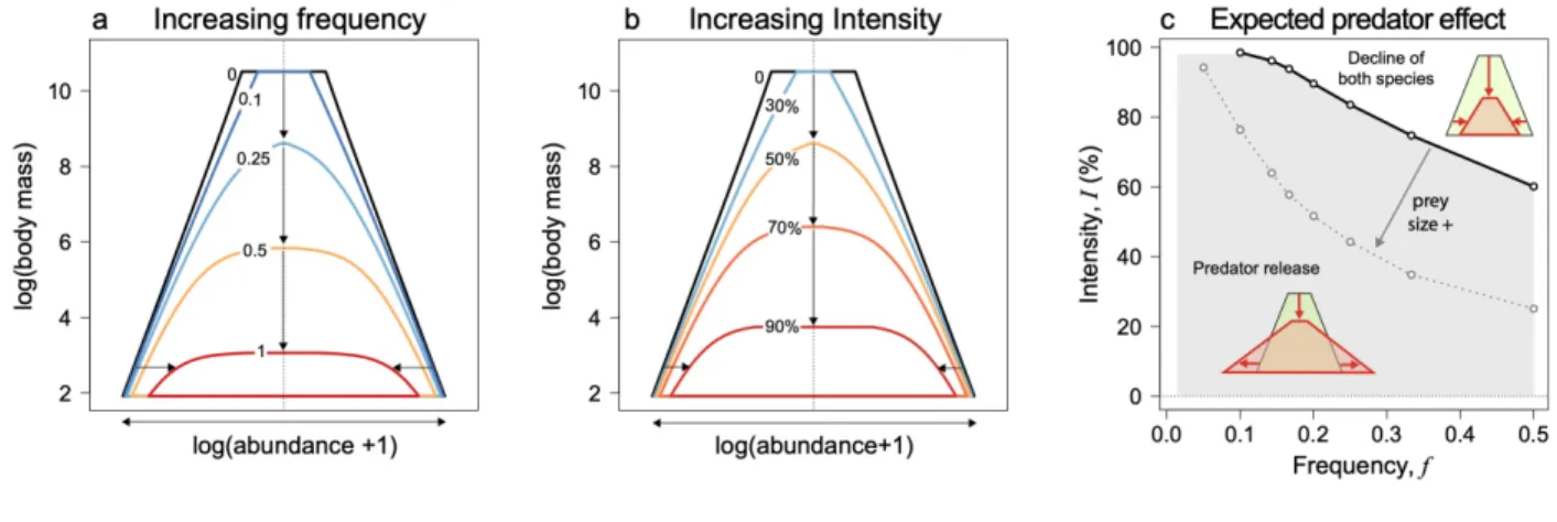
Figure 6: Graphical summary of the effects of disturbances on the shape of size-abundance
622
pyramids. Panels (a) and (b) show size-abundance pyramids for increasing disturbance frequency
623
and intensity, respectively (same analytical results as in Fig. 3a-b). Panel (c) illustrates the expected 624
change in the shape of size-abundance pyramids resulting from a predator-prey dynamic. Lines and 625
points in panel (c) represent isoclines of disturbance regimes {I, T} under which we can expect a 626
predation-release effect leading to wider bases of size-abundance pyramids. Points represent the 627
disturbance intensity for which prey species switch from higher to lower mean abundances at 628
dynamical equilibrium in presence compared to in absence of disturbances, for a given disturbance 629
frequency and a set of predator parameters. Black points are estimated for a smaller prey, i.e. with 630
higher growth rate, than grey points (see detailed method in Appendix 3 and Table S4 for parameter 631
values). 632
633 634
Supporting Information
How pulse disturbances shape size-abundance pyramids
Claire Jacquet1,2*, Isabelle Gounand1,2, Florian Altermatt1,2
1 Department of Aquatic Ecology, Swiss Federal Institute of Aquatic Science and Technology,
Eawag, Dübendorf, Switzerland
2 Department of Evolutionary Biology and Environmental Studies, University of Zurich, Zürich,
Switzerland
* corresponding author: [email protected].
Contents
1. Appendix 1: Analytical derivation of population mean abundance
2. Appendix 2: Detailed methods to produce the theoretical results
3. Appendix 3: Predator-prey model and interaction-release effect
4. Appendix 4: Full experimental methods
5. Supplementary Tables
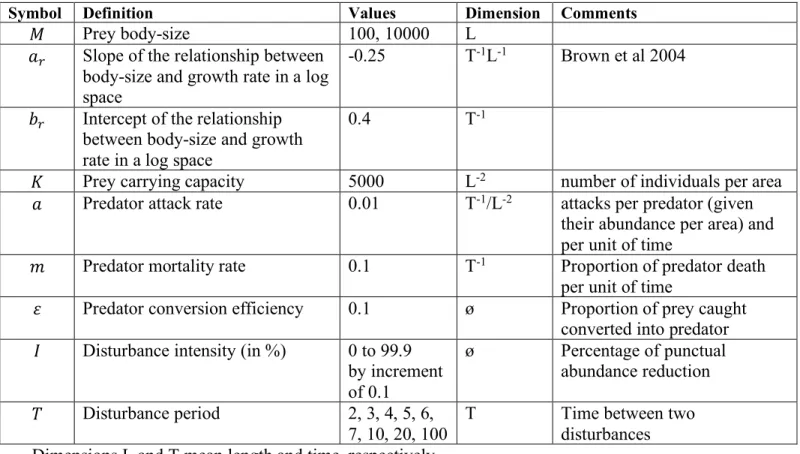
Table S1: Model parameters for the results showed in Figure 3
Table S2: Statistics for the effect of all disturbance regimes on community size-structure Table S3: Model parameters for the results showed in Fig. 5.
Table S4: Predator-prey model parameters for the simulations showed in Figure 6c Table S5: Model parameters for the results showed in Fig. S6.
Table S6: Predator-prey model parameters for the simulations showed in Figs. S9-S11. Table S7: Species information
6. Supplementary Figures
Figure S1: Critical generation time required for long-term population persistence under different disturbance regimes
Figure S2: Experimental results: effect of disturbance frequency on community size-structure and total biomass for different disturbance intensities
Figure S3: Experimental results: effect of disturbance intensity on community size-structure and total biomass for different disturbance frequencies
Figure S4: Comparison between experimental results and model predictions for different disturbance intensities
Figure S5: Comparison between experimental results and model predictions for different disturbance frequencies
Figure S6: Effect of intensity and period variability on size-abundance pyramids Figure S7: Size-structure response to varying slopes and intercepts of the allometric relationship between population growth rate and body-size
Figure S8: Size-structure response to varying slope and intercept of the allometric relationship between population carrying capacity and body-size
Figure S9: Equilibria for varying disturbance frequency, intensity, and prey size Figure S10: Equilibria for varying disturbance intensity, frequency and prey sizes Figure S11: Equilibria for varying prey sizes and disturbance regimes
1. Appendix 1: Analytical derivation of population mean abundance
To investigate the change in community size-structure with disturbances, we derive analytically the equilibrium mean abundance, 𝑁B, of a model in which a population displaying a logistic growth is submitted to recurrent pulse disturbances affecting all species in a similar way. This simple model is described in the methods section (see Fig. 2). The minimal abundance at equilibrium, 𝑁", that is the abundance just after a disturbance, is provided in Harvey et al. (2016), and gives, after simplification:
𝑁" = 𝐾 [1 − 𝐼
1 − 𝑒"F;^ (6)
with 𝑟 and 𝐾 the growth rate and the carrying capacity of the population, respectively. 𝐼 and 𝑇 are the intensity (proportion of abundance reduction) and the period (inverse frequency) of the disturbance regime, respectively.
To get the mean abundance, 𝑁B, we calculate the integral of the abundances between two disturbances at equilibrium, that is between 0 and T, the period of the disturbance regime:
𝑁B = 1
𝑇a 𝑓(𝑡)𝑑𝑡 ;
#
(7)
Here, the function f(t) is the logistic solution, with t the time and 𝑁# the initial abundance:
𝑓(𝑡) = 𝐾
1 + / 𝐾𝑁
#− 13 𝑒
"F+ (8)
To calculate 𝑁B, we note that equation (7) is equivalent to: 𝑁B = 1
𝑇f𝐹(𝑇) − 𝐹(0)h (9)
where F(x) is a primitive of f(t). It can be shown by calculating its derivative that the following function is a primitive of the logistic solution (8):
𝐹(𝑡) = 𝐾 𝑙𝑛(𝐾 + 𝑁#𝑒F+− 𝑁#)
𝑟 (10)
In our case, 𝑁# is the minimal abundance after a disturbance at equilibrium, 𝑁". By replacing equation (6) in (10), and then equation (10) in (9), we obtain the following expression:
𝑁B = 𝐾 j𝑙𝑛(1 − 𝐼)
𝑇𝑟 + 1k (11)
Since we are interested into community size-structure, we want to express mean abundance in function of mean population body-size on a log scale. For that, we assume the following
allometric log-linear relationship between growth rate, 𝑟, and mean body-size, 𝑀, in accordance with the metabolic theory of ecology (Brown et al. 2004; Savage et al. 2004):
𝑙𝑛(𝑟) = 𝑎Fln(𝑀) + 𝑏F (12)
With 𝑎F and 𝑏F being the slope and the intercept of this allometric relationship.
Abundance also scales with body-size on a logarithmic scale (Brown & Gillooly 2003; Brown et al. 2004), then we can assume for carrying capacity:
𝑙𝑛(𝐾) = 𝑎2ln(𝑀) + 𝑏2 (13)
With 𝑎2 and 𝑏2 being the slope and the intercept of this second allometric relationship. By replacing (12) and (13) into (11), we finally obtain:
𝑙𝑛(𝑁B) = 𝑎2ln(𝑀) + 𝑏2+ 𝑙𝑛 j
𝑙𝑛(1 − 𝐼)
𝑇𝑒>P56(m)n oP + 1k (14)
The formula is valid when the expression in parentheses in the right-hand term is positive, which corresponds to the persistence criteria given in equations (2) and (3) of the main text.
We focus here on pulse disturbances to compare the theoretical predictions with the
experimental results. However, press disturbances would have similar effects on size-abundance pyramids. Indeed, if we consider a constant additional mortality rate 𝑚 on the logistic growth, such that population dynamics are described by:
)*
)+ = 𝑟𝑁 /1 − *
23 − 𝑚𝑁 (15)
Then the abundance at equilibrium is 𝑁B = 𝐾 /1 −rF3 and the critical growth rate is 𝑟 > 𝑚. This result demonstrates that press disturbances that are not size-selective will also exclude the large, slow growing species.
2. Appendix 2: Detailed methods to produce the theoretical results
We consider a community made of different co-occurring species constrained by intraspecific competition only. The species populations grow according to logistic functions (equation (1)) with specific growth rates, r and carrying capacities K, and are submitted to disturbances which recurrently reduce population abundances (every T units of time, the period) by destructing a proportion I (the intensity) of all species populations.
Equations (2) and (3) of the main text give the analytical derivation of the critical growth rate above which a population can persist under a given disturbance regime (combination of I and T). This allows to predict the set of disturbance regimes that a population can sustain (Fig. 2b) according to its growth rate, as well as the minimum generation time (1/r) needed to maintain a viable population under a given disturbance regime (Fig. S1).
To analyze the changes in community size-structure driven by disturbance regimes, we consider a set of 1000 co-occurring species, which body-sizes are randomly drawn from a lognormal
distribution of mean 6 and standard deviation 1.5. This provides a range of sizes between 2 and 10 on a logarithmic scale. In an aquatic community for instance, it could correspond to a set of species from bacteria to planktivorous ranging from sizes of 5 µm to 22 mm. We assume a negative allometric relationship between growth rate and body-size (equation 12) with 𝑎F = −0.25, a widely observed value for multiple taxa (Brown et al. 2004), and 𝑏F = 0.4, a value which makes our growth rate gradient ranging approximately from 0.1 to 1, corresponding to common values for microorganisms when day is the time unit. We also derive the carrying capacity K of each species from its body-size assuming a log-linear relationship (equation (13)), with the slope 𝑎2 = −0.75, following a commonly observed value (Brown & Gillooly 2003; Brown et al. 2004), and the intercept 𝑏2 = 10, chosen to have values from 10 to 5000 for K,