Discontinuous shear thickening in the presence of polymers adsorbed on the surface of calcium carbonate particles

HAL Id: hal-01688273

https://hal.archives-ouvertes.fr/hal-01688273

Submitted on 22 Sep 2018

HAL is a multi-disciplinary open access archive for the deposit and dissemination of sci-entific research documents, whether they are pub-lished or not. The documents may come from teaching and research institutions in France or abroad, or from public or private research centers.

L’archive ouverte pluridisciplinaire HAL, est destinée au dépôt et à la diffusion de documents scientifiques de niveau recherche, publiés ou non, émanant des établissements d’enseignement et de recherche français ou étrangers, des laboratoires publics ou privés.

Discontinuous shear thickening in the presence of

polymers adsorbed on the surface of calcium carbonate

particles

Georges Bossis, Pascal Boustingorry, Yan Grasselli, Alain Meunier, Romain

Morini, Audrey Zubarev, Olga Volkova

To cite this version:

Georges Bossis, Pascal Boustingorry, Yan Grasselli, Alain Meunier, Romain Morini, et al.. Discon-tinuous shear thickening in the presence of polymers adsorbed on the surface of calcium carbonate particles. Rheologica Acta, Springer Verlag, 2017, 56 (5), pp.415 - 430. �10.1007/s00397-017-1005-4�. �hal-01688273�

Discontinuous shear thickening in the

presence of polymers adsorbed on the

surface of calcium carbonate particles

G. BOSSIS1, P.BOUSTINGORRY2, Y.GRASSELLI3, A.MEUNIER1, R.MORINI1, A.ZUBAREV4, O.VOLKOVA1

1

Université de Nice Sophia Antipolis, Laboratoire de Physique de la Matière Condensée, CNRS UMR 7336, Parc Valrose, 06108 Nice cedex 2, France

2CHRYSO R&D, 7 rue de l'Europe, 45300 Sermaises, France

3Université Côte d'Azur – SKEMA France – 60 rue Dostoievski – CS30085 – 06902 Sophia Antipolis, France

4Urals State University, Ekaterinburg, Lenin Ave, 51, Russia

Abstract

In the presence of dispersant molecules currently used in cement industry and based on polyethylene oxide (PEO) we found a strong discontinuous shear thickening (DST) at high volume fraction in suspensions of calcium carbonate particles. The transition was reversible and the critical shear rate and shear stress for which this instability appears are reported versus the volume fraction of particles. A model of repulsive forces between polymers, taking into account the thickness of the polymer layer and the density of adsorption on the surface of the particles, can explain the differences of critical stresses observed between these three dispersant molecules. In particular it explains why a small polymer densely adsorbed can be more efficient to repel the transition at higher stress than a larger molecule less densely adsorbed. Above the transition, we find that the suspension presents a special kind of stick-slip instability with even the presence of a negative shear rate under constant applied stress. A model is proposed which well predicts this regime by taking into account both the inertia of the apparatus and the viscoelasticity of the suspension.

I INTRODUCTION

Shear thickening, either continuous or discontinuous has long been known in the area of concentrated suspensions of solid particles. Continuous shear thickening is usually due to the formation of clusters of particles occurring when the shear forces dominate the repulsive ones. Repulsive forces can be indirect like those due to Brownian motion which are proportional to kT/R -where R is the radius of the particles- or can derive from a potential like, for instance, Debye-Huckel forces. When the hydrodynamic stress

overcomes the Brownian one and/or the stress due to the short range repulsive forces, the viscosity begins to increase and will tend towards the one of a suspension of hard spheres. This behavior was well evidenced through numerical simulations of particles with hydrodynamic interactions, (Melrose et al. 1996; Bossis and Brady 1989). The observation of this general behavior can be hidden by the existence of a yield stress, due to frictional contacts in the presence of gravity for large particles or to Van Der Waals attractive forces for colloidal particles (Brown et al. 2010). On the other hand, a continuous increase of viscosity can be followed by a discontinuous jump of viscosity. It can happen through an order-disorder transition as observed on a monodisperse suspension of micron size particles (Hoffman 1972; Hoffman 1982) where, before the transition, the particles are ordered in hexagonal layers which flow, passing one over the other. This is not the case in blends of particles where there is no preexisting ordering and, in this case, the transition results from a sudden aggregation driven by a parameter still expressing the balance between shear forces and stabilizing forces (Chaffey and Wagstaff 1977). In suspensions were the repulsive forces between particles are due to ionic layers and can be controlled either by the pH or the addition of salt the critical shear rate of the DST transition was clearly increasing with the range of the interparticle force (Boersma et al 1990, Franks et al 2000). A relevant hypothesis,which was confirmed by numerical simulations(Mari et al, 2014), is that discontinuous shear thickening occurs when the surfaces of the particles come into contact generating a solid friction which creates a percolating network of particles whose rigidity is produced by the contact forces. This solid network resists to the strain and thus reduces the shear rate even if the stress increases, giving a negative differential viscosity in an imposed stress experiment. The breaking and reforming of this network was supposed to be responsible for the fluctuations of velocity observed at constant stress (Frith et al. 1996). In this approach it is supposed that the suspension remains spatially homogeneous and, actually, this is what is observed in simulations where contact forces are introduced (Mari et al. 2014). Also, in a recent work, using a confocal microscope and fluorescent molecules in a cone-plate geometry (Pan et al. 2015) the suspension was found to remain homogeneous, even in the DST domain. Nevertheless, in the presence of a negative differential viscosity the system is unstable and should lead to an inhomogeneity in the local structure which can manifest by a shear localization in a thin layer and two immobilized solid parts. This behavior was observed in laponite suspensions together with stick-slip oscillation of the stress at constant shear rate (Pignon et al.1996) but, in this case, it was associated with the presence of a static yield stress and not to the DST transition. A model, with a local order parameter depending on the stress, was introduced (Nakanishi et al. 2012) to reproduce the instability; it involves the inertia of the fluid and predicts a change of frequency of the stick-slip oscillation with the height of the cell. Although the structural variable introduced in this model was not specified it could be identified to the fraction of frictional contacts (Mari et al. 2014). Another approach of DST, (Wyart and Cates 2014), not involving inertia, was based on a crossover between two states, one where particles are in friction and the other where they are lubricated. The transition from one state to the other was ruled by the balance between shear and repulsive forces. An appropriate dependence of the jamming volume fraction relatively to the fraction of frictional contacts allowed them to find a "phase diagram" with a DST domain where the shear rate should

fluctuate between two values. A similar "phase diagram" was also proposed (Bi et al. 2011) with the existence of a "shear jammed domain". Giant fluctuations between two values of stress for a constant applied shear rate were observed (Lootens et al. 2003) with a suspension of monodisperse silica spheres. Recent measurements on silica spheres of different diameters (Guy et al. 2015) support the theoretical approach of crossover between two states. Most of the experimental results report that the DST transition is reversible (Marazano and Wagner 2001; Nenno and Wetzel 2014; Neuville et al. 2012), meaning in particular that two successive ramps of stress will give the same rheogram. Nevertheless, in a large gap cylindrical Couette cell, it was observed (Fall et al. 2015) that DST was associated with a large migration of the particles made of polystyrene beads of diameter 50µm, towards the outer cylinder and so was not reproducible. In a recent paper based on a cornstarch suspension the analysis of the density by magnetic resonance imaging lead these authors to the conclusion that the two states picture of (Wyart and Cates 2014), associated with the S-shape of the shear stress versus shear rate, was irrelevant (Fall et al. 2015). Another puzzling observation (Fall et al. 2008), still with a cornstarch suspension, was that the critical shear rate for DST was depending linearly on the thickness of the gap in a plane-plane geometry whereas it was constant in the presence of a surplus of paste around the plates. The role of the interface is important because it generates a confining capillary pressure preventing the particles to escape from the fluid during the dilation of the network of particles (Cates et al, Brown and Jaeger 2012) and could partly explain the observations made on cornstarch suspensions.

From these contradictory observations, it appears that, despite the fact that the phenomenon of DST was known for a long time, it is still poorly understood because it is at the interface between granular and suspension rheology. It certainly needs more experimental results with different systems and geometry in order to have a general picture of the phenomenon. As already mentioned, the onset of DST is ruled by a balance between shear forces and repulsive forces. If the first ones dominate, then the surface of the particles can come into contact and produce the DST phenomenon. Our aim in this paper is to look for the DST phenomenon in suspensions where the particles are covered by a polymer layer and to relate the characteristics of the polymer layer to the onset of DST. For this purpose, we have chosen a suspension of calcium carbonate particles in the presence of different dispersant molecules which are currently used in cement industry. We shall see that, thanks to these molecules and to the polydispersity of the particles we can reach volume fraction as high as 69% with still a negligible yield stress. These supensions present a strong DST transition with an important decrease of the shear rate at a critical stress. Knowing the main characteristic of the polymer and the ionic content of the suspension we shall compare the repulsive force to the one applied on the suspension by the shear in order to evaluate the critical stress for DST. These theoretical values will be compared with the experimental ones for the three molecules we have used. In the last section we shall present a model to explain the origin of a regular stick-slip behavior observed when the stress is maintained at a constant value just above the critical one.

II MATERIALS

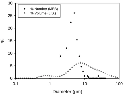
The suspension we have chosen is made of commercial calcium carbonate particles (BL200 from Omya). Calcium carbonate particles are used industrially to coat paper; they are also used as a filler to improve the mechanical properties of thermoplastics. In our case this mineral was chosen as a model of more complex materials like cement where the interactions between the calcium ions and the polyelectrolytes play a major role to reduce the yield stress and facilitate the flow of cement paste and concrete. The rheology of suspensions of CaCO3 in water was previously studied in the presence of sodium polyacrylate as dispersant (Deng et al. 2010) and also in the context of shear thickening by Egres et al (Egres and Wagner 2005). In this last case the particles were acicular and dispersed in polyethylene glycol and the emphasis was on the effect of different aspect ratios on shear thickening and DST. The shape of our particles is irregular but more or less rhomboidal as can be seen on the picture (Fig.1) obtained by electronic microscopy. In Fig. (2), the size distribution in volume obtained by light scattering (with the Mastersizer 2000) is represented by the open triangles, it shows two populations, one of them being formed by particles of diameter below one micron. The second curve with solid diamonds was obtained by classifying 350 particles from MEB pictures. We found a proportion of about 30% of particles smaller than one micron which we did not take into account because, as we shall see later, the jamming transition is related to the formation of a percolation network across the cell which likely does not involve the smallest particles. The average size of particles above 1 micron is 5.5 micron. We did not use the size distribution obtained by light scattering because the change to a number distribution is not guaranteed at all, especially with particles of irregular shape with two modes in the size distribution.

Diameter (µm) 0.1 1 10 100 % 0 5 10 15 20 25 30 % Number (MEB) % Volume (L.S.)

Fig.2 Size distribution obtained by counting the particles above 1µm from MEB pictures and from light scattering (L.S.) with Mastersizer 2000 from Malvern

The density of the particles was 2525kg/m3 and the measurement of their specific surface by BET gave 0.88 m²/g. The dispersant molecules were two comb like polymers called PCP45 and PCP114 with a polymethacrylate backbone and side chains made of polyethylene oxide (PEO) and a small molecule where the backbone was replaced by a polyphosponate group and called PPP44. The numbers 45,114, 44 in the name, indicate the number of units in the PEO chain. The average number of monomers between two side chains was N=5 both for PCP45 and PCP114.

Fig. 3 Sketch of the structure of the three polymers

The three molecules are represented in Fig.3 to figure out their respective length. The molar mass of a PEO chain with 45 units was 1804 g/mole and the PCP45 has 10 side chains with a total molar mass of 25000 g/mole. The adsorption isotherms were obtained from the measurement of the total organic carbon at a pH of 9.3 imposed by the solvation of calcium carbonate. The plateau of the adsorption curve is obtained from a fit by a Langevin law; it gives 0.14, 0.06 and 0.23 segments/nm2 respectively for the

PCP45, PCP114, PPP44 (Morini 2013). We call a segment a side chain together with the unit of the skeleton to which it is attached, but for the last polymer PPP44, a segment corresponds to the whole molecule. We note that the density of adsorption is the largest for the molecule PPP44 having a single side chain, and that, among the two others, the longer chain corresponds to a density which is more than two times smaller because of its larger gyration radius. Supposing that all the side chains are equidistant, the average distance, s, between two chains is given by

s

=

1/ n

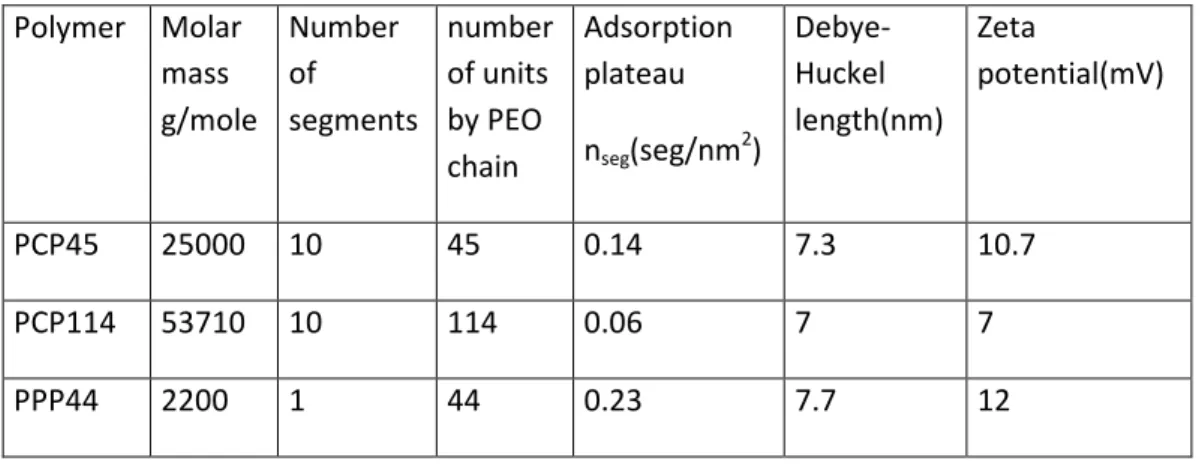
_seg with nseg the

number of segments per nm2. Even if this hypothesis is quite questionable, since in PCP45 and PCP114 the PEO chains are not free but ten of them belong to a given molecule, it gives an idea of the organization of the PEO chains on the surface of the particles. The data corresponding to these three molecules are reported in the table I. Table I: Main characteristics of the system polymer/particles

Polymer Molar mass g/mole Number of segments number of units by PEO chain Adsorption plateau nseg(seg/nm 2 ) Debye-Huckel length(nm) Zeta potential(mV) PCP45 25000 10 45 0.14 7.3 10.7 PCP114 53710 10 114 0.06 7 7 PPP44 2200 1 44 0.23 7.7 12

The Debye Huckel length was obtained from the different ionic concentrations in the suspension of CaCO3 particles at equilibrium corresponding to a concentration of

dispersant of 0.2%wt relatively to the mass of the particles (Morini et al. 2013). The zeta potential was measured on the smallest particles after sedimentation and was found around 10mV (c.f. Table1).

III- Experimental determination of the jamming

characteristics

The experiments were mainly done on a rheometer MCR301 from Anton Paar. The geometry used was a plate- plate geometry with a serrated profile to prevent slipping of the paste; the diameter of the plate was 40mm. In the plate-plate geometry we used a cover and a water trap in order to prevent evaporation during the measurement which were realized at 20°C. The experiments were conducted with a pre-shear of 3mn at

γ

_ɺ

=5 s-1 and a rest time of 30s before the ramp of stress with a typical rising time of 20 Pa/min which was chosen to obtain steady state results and being still fast enough to be able to do the experiment without drying. In Fig. 4 we present the stress versus shear rate curves for a suspension prepared at a volume fraction Φ=0.6. The upper curve corresponds to the suspension without any dispersant and shows an important yield

stress. The three lower curves show the rheogram for a suspension adjuvanted with each of the three polymers at a concentration corresponding to the beginning of the adsorption plateau. We can see that the yield stress has almost disappeared for the PCP45 and the PCP114 and that there is practically no difference between them; the curve for PPP44 is slightly different with a yield stress around 1Pa and a smaller final viscosity. Also the suspension is slightly shear thickening. It is worth noting that if we decrease the concentration of polymer by a factor of two, the yield stress remains low but the shear thickening behavior is much larger.

Shear Rate (s-1)

1 10 100

S

h

e

a

r

S

tr

e

s

s

(

P

a

)

0.1 1 10 100 1000 10000 Without Polymer 0.2wt% PPP44 0.12wt% PCP114 0.12wt% PCP45

φ

V

=0.6

Fig.4 Comparison of the rheograms- shear stress versus shear rate- of a suspension of calcium carbonate at volume fraction Φ=60% without dispersant (upper curve) and with each of the three polymers

At higher volume fraction and keeping a high concentration of polymer: c=0.2%wt to be sure that we are well on the adsorption plateau, we obtained the evolution shown in fig.5 for the PCP45. At Φ=62% we observe a quite strong shear thickening but the rheogram remains smooth; at Φ= 63% the slope is steeper and we begin to observe a few sudden decrease of the shear rate; this is amplified at 64% and finally at 65% we have the onset of a negative differential viscosity followed by a quasi-vertical evolution corresponding to an infinite differential viscosity. This behavior is rather different to the one observed on other suspensions showing DST where, after the jamming transition, the differential viscosity recovers a value close to the one observed before the DST (Pan et al. 2015).

Shear Rate (s-1) 0 100 200 300 400 500 S h e a r S tr e s s ( P a ) 0 100 200 300 400 62% 63% 64% 65%

Fig.5 Evolution of the rheology of the suspension of calcium carbonate at different volume fractions adjuvanted with PCP45 at 0.2% wt. The increase of volume fraction goes from the right to the left

All the suspensions were prepared in the same way: small quantities (typically 50g of CaCO3) were mixed on a vortex during 5mn with the water adjuvanted by the fluidizer, then the suspension was placed during 15mn in an ultrasonic bath and still placed 5 min on the vortex. The more important cause of uncertainty was the precision of the filling process since the suspension must match as well as possible with the rim of the upper plate which is not so easy with serrated plates. Possible drying on the edge of the plate can also be a source of error so it was systematically checked by repeating the same experiment as the first one from time to time; if the result was different, another sample was loaded. Another possible cause of error is due the wall slip which manifests by different rheological curves for different gaps; in this case it is possible to remove the slipping velocity and obtain the right shear rate (Chryss et al. 2005; Buscall 2010). In our case we have done the experiments with PCP45 for three different gaps: 0.5mm, 1mm, 1.5mm taking 10 curves for each gap. The maximum difference between the three average values was of 13% and without tendency. As examples we have shown the curves in Figs (6) and (7) for three different gaps and two different molecules: PCP45 and PPP44. In Fig.6, up to the jamming transition, the curves are practically superposed; it is after the transition that the behavior becomes quite different with an amplitude of the fluctuations which is much smaller for the gap of 0.5mm than for the two other ones. For the PPP44 the difference between the curves obtained with different gaps is small and not continuous with the gap since the lower curve corresponds to a gap of 0.5mm, the middle one to 1.5mm and the upper one to 1mm. Above the transition the oscillations of the shear rate are still different but there is no clear conclusion to draw since now it is the gap of 0.5 mm which shows the higher amplitude. We have also reported in Fig. (6) a curve obtained with smooth plates and a gap of 1mm; this curve is not different from the one obtained with serrated plates except that it does not show a jamming transition, but a monotonic increase of the shear rate till a point where pasty

granules appear on the rim of the plates followed by an expulsion of the paste. It then appears without any doubt that, below the jamming point, there is no slip on the walls and that for the manifestation of the jamming, a rough surface is needed. Still, before jamming, there is a shear thickening part which should be taken into account with the help of the Mooney-Rabinovitch equation as we shall see below.

Shear Rate (s

-1

)

0 10 20 30 40

S

h

e

a

r

S

tr

e

s

s

(

P

a

)

0 20 40 60 80 100 120 140 1mm, smooth 1mm 1.5mm 0.5mm

Fig.6 Three ramps of stress with different gaps: 0.5, 1, 1.5mm at Φ=68% with fluidizer PCP45 and serrated plates. The curve with open square symbols is obtained with smooth plates

Shear Rate (s-1) 0 20 40 60 80 S h e a r S tr e s s ( P a ) 0 50 100 150 200 250 300 1.5mm 0.5mm 1.0 mm

Fig.7 Three ramps of stress with different gaps and serrated plates at Φ=68% with fluidizer PPP44. The middle curve with crosses corresponds to 1.5mm

Another point which needs consideration is the thixotropy. Since the phenomenon of shear thickening and jamming is provoked by the building of aggregates of particles followed by the percolation of a network of particles in frictional contacts, it is worth

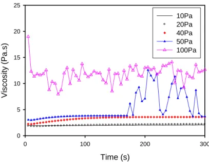
looking at the time scale needed to form these aggregates at different imposed stress and correlatively to the effect of the rising time of the stress on the shear stress versus shear rate curve. In this aim we have to look at the shear creep rate coefficient where we follow the evolution with time of the viscosity after imposing a constant shear stress at t=0; this is the equivalent of the shear stress growth coefficient for an imposed shear rate experiment. We have plotted in Fig.8 this time dependent viscosity for the PCP45 and five values of the stress: σ=10, 20, 40, 50, 100 Pa. The three first values are below the jamming point; the value of σ=50Pa is slightly above the critical stress and σ=100Pa is well inside the jammed state. We first see that, for the two lower stresses σ=10Pa and σ=20Pa, the steady state is reached quickly, whereas it takes about 2 min for the stresses of 40 and 50Pa. The two viscosities at σ=10 Pa and σ=20 Pa are very close from each other, showing that we are still in the linear regime. For σ=40Pa, which is in the shear thickening domain, the viscosity increases significantly with time from 2.2 Pa to 3. 8Pa.s in about 2mn. For σ=50 Pa the behavior is quite similar except that we observe an incursion in the jamming domain with strong oscillations of the viscosity showing that σ=50 Pa is actually just above the critical shear stress. For the highest stress, σ=100Pa, the viscosity has jumped to a higher average value and is fluctuating with a large amplitude but the equilibrium time is small (less than 10s) and corresponds to an initial decrease of the viscosity. The important point for our discussion concerning the critical shear rate and critical stress in relation with the type of superplasticizer molecule is to know if our ramp of stress at a rate of 20 Pa/min corresponds to an equilibrium sate. In this aim we have plotted in Fig. 9 three curves corresponding to ramp of stresses realized with different rising times, namely 200 Pa/min, 60Pa/min and 20 Pa/min. On the same graph we present in black the points corresponding to the evolution of the shear rate with time at a constant applied stress which can be deduced from Fig.8. The last values on the left correspond to the equilibrium values. We see that the ramp of stress at 200 Pa/min is clearly out of equilibrium and that the jamming point is delayed at higher stress and shear rate because the structure did not have time to build. The curve at 200Pa/min is close to the first values of the shear rate obtained after the imposition of a constant stress at t=0. The curves realized at 60 Pa/min and 20 Pa/min begin to diverge at higher shear rates and are on the left extremity of the horizontal set of points corresponding to the equilibrium sate for 10 and 20 Pa. It remains a 10% difference at σ=40 Pa between the equilibrium value of the shear rate and the one obtained with a rate of 20Pa/min that we have used for all the experiments. As already stated at the beginning of section III, the choice of 20Pa/min is a compromise between the drying time and the time needed to reach the equilibrium. It is worth noting that the critical stress obtained for the ramp at 20 Pa/min is well the equilibrium one as attested by the behavior of the shear rate at σ=50 Pa in Fig.8 and we shall see in section IV.2, that the stress is the control parameter of the jamming transition. The residual difference between the equilibrium shear rate and the one measured with a ramp of stress at 20Pa/min remains quite small (<10%), and concerns only the value of the critical shear rate (Fig.16) which is likely overvalued of approximately 10%. This should be kept in mind but has no practical impact, since the aim of this figure is mainly to show the difference of behavior between the different superplasticizer molecules for experiments realized in the same conditions which are clearly close to the equilibrium ones.

Time (s) 0 100 200 300 V is c o s it y (P a .s ) 0 5 10 15 20 25 10Pa 20Pa 40Pa 50Pa 100Pa

Fig.8 Creep rate curves at different imposed stresses. PCP45, φ=68%

Shear Rate (s

-1

)

0 5 10 15 20 25 30

S

h

e

a

r

S

tr

e

s

s

(

P

a

)

0 20 40 60 80 100 120 20 Pa/mn 60 Pa/mn 200 Pa/mn 10 Pa 20 Pa 40 Pa 50 Pa 100 Pa 10 Pa 20 Pa 40 Pa 50 Pa 100 Pa

Fig. 9 Ramps of stress at different rising rates, compared to the evolution of shear rate at different imposed stresses presented in Fig. 8 ;the time is growing from right to left.

Above the jamming transition the shear rate oscillates between values whose average can remain constant or not. The two cases are illustrated in Fig.10 for a ramp of stress at a volume fraction Φ=68% and with the molecule PCP45. During the first ramp of stress the average value of the shear rate oscillations remains constant at a value close to 5s-1. On the contrary, for the second ramp of stress, the oscillations begin in the same way but progressively shift towards higher values and if we still increase the stress we observe that the suspension is getting out of the gap. As shown previously (Cates et al. 2005, Brown and Jaeger, 2012), it happens when the radial normal force generated by the dilatancy of the suspension during the jamming state is no longer compensated by

the capillary pressure P=γ/R -where R is the radius of the particle and γ the interfacial tension. In this case the particles begin to be ejected from the suspension with, correlatively, air entering inside the suspension. It is also worth noting that, if the fluctuations take place around a constant average value, there is no hysteresis when the stress is decreased. We have also made some measurements with the suspension extending outside the interface between the two plates; the jamming transition still exist but is quite different (Fig.11): there is no abrupt decrease of shear rate but a beginning of fluctuations at about the same stress than in conventional filling, followed by much larger fluctuations at stresses above 120Pa. Also the hysteresis during the descending ramp was quite large and the second ramp of stress did not show the same big fluctuations as the first one. All these observations confirm that if the particles are not confined by the capillary pressure they escape out of the gap between the plates.

Shear Rate (s-1) 0 5 10 15 20 S h e a r S tr e s s ( P a ) 0 100 200 300 400 1st ramp up 2nd ramp up

Shear rate (s-1) 0 5 10 15 20 25 S h e a r s tr e s s ( P a ) 0 50 100 150 200 First ramp up First ramp down Second ramp up

Fig.11 Same as Fig.10 but with the suspension extending outside the gap between the two plates In the following, the comparison of critical shear rates and critical stresses between the three molecules are obtained from experiments made at 20°C in serrated plate-plate geometry with a gap of 1mm and a rate of increase of stress of 20 Pa/mn in a stress controlled mode. Experiments made in the shear rate controlled mode show, at the critical shear rate, a huge jump of stress which overcomes the capacity of the rheometer but the value of the critical shear rate was well consistent with the one obtained in stress controlled mode.

IV- Comparison of the jamming point between the

three molecules

IV-1 Experimental results

Our aim was to record the critical shear rate and critical stress for the three different polymers presented in section II versus the volume fraction. In Fig 12 we have plotted typical results at Φ=68% for the three molecules. We see that the two comb polymers show practically the same rheology with no yield stress, a quasi-Newtonian rheology below 20 s-1and an abrupt jamming, followed by a vertical increase of stress at constant average shear rate. The behavior of the suspension incorporating the small molecule PPP44 is very different: the critical shear rate and critical stress are much higher and the transition is preceded by a shear thickening state. Since we have a shear thickening part we have used the Mooney-Rabinovitch correction which relates the true yield stress, τ, to the stress, τN, given by the software for a Newtonian fluid:

The resulting correction is shown by the solid lines for the PCP114 and by the dotted line for the PPP44. The correction is about 20% for the PCP114-and this is also true for the PCP45- but larger for the PPP44 which presents a stronger thickening behavior before jamming. The values of the critical stresses reported in Fig.14 were all determined in this way. Shear rate (s-1) 0 10 20 30 40 50 60 S tre s s ( P a ) 0 50 100 150 200 250 300 PCP114 PCP114 Corrected PPP44 PPP44 Corrected PCP45

Fig.12 Comparison of the jamming transition for the suspension of CaCO3 at Φ=68% for the three different molecules. The solid and dotted lines are obtained from Mooney-Rabinovitch correction For the three molecules we note that we do not observe a S-shape for the stress versus shear rate but rather a shear rate which decreases abruptly and then fluctuates around a constant value lower than the critical shear rate. The same observation was made (Frith et al. 1996, Laun 1994) on suspensions of latex particles stabilized by ionic charges. The comparison of the critical shear rates for the three molecules is represented in Fig. 13 for different volume fractions; the uncertainty bar is the root mean square error over at least 10 different experiments.

Volume Fraction (%) 64 65 66 67 68 69 70 C ri ti c a l S h e a r R a te ( s -1 ) 0 20 40 60 80 PCP45 PCP114 PPP44

Fig.13 Evolution of the critical shear rate with the volume fraction for the three molecules

Volume Fraction (%) 64 65 66 67 68 69 70 C ri ti c a l S h e a r S tr e s s ( P a ) 0 50 100 150 200 PCP45 PCP114 PPP44

Fig.14 Evolution of the critical shear stress with the volume fraction for the three molecules We note that the two comb polymers have practically the same critical shear rates and that the DST transition begins at a volume fraction of 65%. With the PPP44, the DST starts at 67% and with a much higher critical shear rate. For the three molecules the decrease of the critical shear rate with the volume fraction is practically linear with the extrapolation corresponding to a completely jammed state at a volume fraction of 70%. The other representative quantity for this transition is the critical shear stress which is represented in Fig.14. We see that the critical stress is much higher for the small polymer PPP44 than for the two others comb polymers which have the same value 45

±

5Pa. Another striking difference is that for the comb polymers the critical stress does not depend on the volume fraction whereas it clearly decreases with the volume

fraction for the PPP44. In the following section we are trying to explain these different behaviors by looking at the different forces acting between the surfaces of the particles.

IV -2 Model used to predict the DST transition

The common thinking about DST is that it results from a change of structure which happens when the hydrodynamic forces dominate the repulsive ones. Such approach (Boersma et al. 1990) was used for particles stabilized by their ionic layer. The repulsive force between two spherical particles in the presence of an ionic double layer is given by:

(1)

where ε0 is the vacuum permittivity εr the relative dielectric constant , ζ, the zeta

potential, R the radius of the particles, κ is the reciprocal Debye double layer thickness and h the separation between the solid surfaces of the two particles. The plus sign in the denominator of Eq. (1) corresponds to a constant potential and is taken if the charges have time to rearrange when the distance between the surfaces changes, which is the case in water. The value of the double layer thickness depends on the concentration of the different counter ions and was given in table I, as well as the zeta potential

The expression of the hydrodynamic force is not so easy to obtain. We know that, for two particles at rest in a shear rate

γ

_ɺ

with a suspending fluid of viscosity µ, the order of magnitude of the hydrodynamic force will be:

(2)

The lubrication force is obtained by multiplying Eq. (2) by R/h but this force, which generates the divergence of the viscosity at high volume fraction, should not intervene in a balance of forces where particles are considered at rest; furthermore this force is repulsive on the compression axis. Actually in a dense suspension the hydrodynamic force exerted between two given particles is mediated by all the surrounding ones; which can be represented by introducing in Eq. (2) the real viscosity of the suspension rather than the one of the suspending fluid. If the viscosity scales as µR/h, then we recover the previous approach (Boersma et al. 1990) which gave a correct estimation of the critical shear rate for particles stabilized by an ionic layer. A more evident approximation of the hydrodynamic force is obtained by considering the applied stress instead of the shear rate, then we have simply:

(3)

where σ is the applied stress and 4R2 the typical cross section around two given particles.

At very short distance we consider the hydration force resulting from the interaction between two layers of water molecules which are usually adsorbed on the surface of mineral particles (Manciu et al, 2001)]:

with (4)

Ah is the Hamaker constant, e - the Neper number and λ− the decay length that can be

taken equal to 0.3nm. This force represents the short range repulsive barrier. The attractive Van der Waals force is also proportional to the radius of the particles:

(5)

The value of the Hamaker constant for the interaction between two calcium carbonate particles in water was: Ah= 2.23 10

-20

J (Hough and White 1980).

The repulsive force between the two layers of polymers respectively adsorbed on each particle is more awkward to calculate. The first difficulty is to estimate the thickness of the polymer layer. From the adsorption isotherm we know that, for the three molecules we have studied, the saturation corresponds to a monolayer, but the thickness of this monolayer depends on the model used to describe the interactions between the monomers. For the PPP44 which is essentially a polyethylene oxide chain, the water is a good solvent with a Flory parameter:

χ ≈

0.36

at room temperature (Pedersen and Sommer 2005) and the end to end distance is given by δe=b P

3/5

where b is the Kuhn length and P the number of monomer. Ab initio calculations (Mark and Flory 1965) give <δe2>=12.3 P.l2=P.b2 with l=0.15nm the average length of a bond; it gives b=0.526nm.

This value corresponds also to the one: b=0.37 2 found by numerical simulation (Lee et al. 2008); then in a good solvent and with P=44 we get δe=4.96nm for an isolated

chain of PPP44. Actually the thickness of the layer should be larger since in the case of a brush organization, which applies for the PPP44 where each chain is individually attached on the surface by its phosphonate group, the entropic repulsion between the monomers of different chains will lead to an extension of the polymers. Following the self-consistent field theory (SCF), (Milner et al. 1988) we should have:

(6)

where s=1/ n_seg is the average distance between grafted chains. Except for the prefactor 12/π2 and the fact that χ was taken equal to zero,this expression is the same as the one previously derived by De Gennes(De Gennes 1987).

Applying Eq. (6) with the values of s reported in table 1, we obtain respectively δPPP44=6.1nm δPCP45=5.4nm and δPCP114=10.1nm. It should be noted that the theory is

the conformation of the skeleton on the particle surface and the resulting geometric constraints on the side chains may result in a different extension. The size of PCP comb polymers of similar molecular masses as ours was characterized (Borget et al. 2005), by different techniques. These authors have found all of them in the flexible backbone wormlike regime, (Gay and Raphael 2001), in which these polymers are considered to be made of blobs of size δ containing n_c = P / Nside chains with N the number of monomers along the backbone between two chains (N=5 for the PCP45 and PCP114). This blob size, was well represented by: δ'=b. P7/10 N-1/10. If we consider the diameter of the blobs as the thickness of the adsorbed layer, we find δ'PCP45=6.2nm instead of 5.4nm

and δ'PCP114=11.9nm instead of 10.1nm. The difference is less than 15% and, as we shall

see later, it is note the absolute value of the layer thickness which is important but rather its relative compression; so, for the sake of coherence with the expression of the energy of a compressed layer, we shall keep Eq. (6) for the estimation of the layer thickness.

In the SCF model (Milner et al. 1988) the energy of two compressed brushes per unit surface between two planes separated by a distance h is given by:

with (7)

In the De Gennes model the density profile is step-like instead of parabolic and the energy is different:

with (8)

The resulting polymeric force between two spherical particles is obtained from the Derjaguin approximation (White 1983):

(9)

It is worth noting that in these models the polymers are not interpenetrating and that these predictions are quite well confirmed by surface force apparatus measurements (Tadmor et al. 2003; Taunton et al. 1988). Taking s given in table 1 and δ given by Eq. (6) we can now compare the repulsive force to the Van der Waals one and also to the Debye Huckel force.

Separation (nm) 0 2 4 6 8 10 12 F ( p N ) -2000 -1000 0 1000 2000

Van Der Waals De Gennes Milner

Fig.15 Comparison of the different forces between two particles coated by PPP44. Van der Waals :Eqs (4)-(5); De Gennes model: Eqs (4)-(5)-(8)-(9); Milner model: Eqs (4)-(5)-(7)-(9)

σ(Pa) 0 20 40 60 80 100 120 140 h / δ 0.0 0.5 1.0 1.5 2.0 PPP44 PCP45 PCP114

Sigma (Pa) vs Col 5 1.19

Fig. 16 Equilibrium distance between the particle surfaces versus applied stress; the distance is normalized by the thickness of each respective layer;the repulsive force is taken from Eq.(7) As can be seen in Fig. 15 both models predict quite similar repulsive force which largely dominate the attractive Van Der Waals force and is then very efficient to suppress the yield stress. The Debye Huckel force is also completely negligible compared to the force induced by the polymer layer and this is verified for the three molecules. In Fig. 16 we have plotted the point of equilibrium separation between the surfaces obtained by equating to zero the total force, including the shear force Eq. (3). This separation is normalized by the thickness of the polymer layer and is represented versus the applied stress. We see that the separation distance drops more quickly for the two PCP polymers than for the PPP44 molecule. The pressure exerted on the polymer heads by the compression of the layer is Pp=Fp/Sp with Sp≃2πR(δ-h/2) the surface of the polymer

brushes which are in contact. The repulsive force Fp is proportional to R times δ (Eqs. (9)

and (8)) or equivalently to R times P (Eqs. (9) and (7)), so finally this pressure does not depend on the radius of the particles neither on the thickness of the polymer layer but rather of its relative compression. We shall suppose that, above a given compression, of the polymer layer we have a sudden desorption of the polymer which will allow to the particles to come in frictional contact thus generating the DST transition. This hypothesis of dynamic desorption under compression was made (Klein et al. 1994) to support the observation that, above a given compression of the polymer brushes, the shear force between two mica plates measured by surface force apparatus was raising by several orders of magnitude. It was confirmed later in other experiments (Raviv et al. 2001); for a review see also (Klein 2013). If we take as a reference the PPP44 molecule, since its unique chain makes the force model more reliable, the average experimental value of the critical stress σc =155 Pa for Φ=68% would correspond to a value of h/δ= 1.19 in the

Milner model (cf. Fig.16). If we conclude that this compression ratio of the PEO chain corresponds to a threshold for the layer stability, then we can tentatively use the same criteria for the two comb polymers. For this same value of h/δ we obtain σc =42Pa for

the PCP114 and σc=76 for the PCP45 compared to the experimental value of 45

±

5Pa

for both molecules. The larger value for the PCP45 could come from the fact that we have overestimated the Flory parameter when taking χ=0.36 for the three molecules: the presence of the PMMA skeleton which is more hydrophobic than the PEO chain will likely increase χ, especially for the PCP45 where the ratio of the molar mass of the skeleton over the side chains is the larger one. For instance, taking χ=0.44 for the PCP45 would give the same critical stress for both PCP45 and PCP114. It is also worth noting that using the De Gennes model we obtain similar predictions; for instance, with χ=0.36 for the three molecules, the ratio of compression giving σc=155Pa for the PPP44 is

h/δ=1.28 and we obtain σc=70 Pa for the PCP45 and σc =34 Pa for the PCP114.

If we neglect the Debye Huckel contribution to the force, the condition relating the percentage of compression to the critical stress, σc, is readily obtained from the

condition of a zero total force. In the case of the De Gennes model which gives the simplest expression, using Eqs (3), (5) and (8) we obtain:

(10)

With and

The critical value of u is a parameter which is the ratio of compression of the polymer above which we expect its desorption; it is an unknown to be determined from the measurement of σc. This value is likely related to the adsorption energy of the polymer

head, which is, in our case, of electrostatic origin. From Eq. (10) we see that, if we want a high critical stress, we need to have a high ratio (δ/s) of the thickness of the polymer layer to the average distance between two terminal heads of polymer. Also for a given ratio, δ/s, it is better to have a small polymer chain than a long one. This last assertion should be moderated by the fact that the force model is based on the notion of blobs

which becomes less and less realistic for small polymer chains. In the derivation of the equilibrium separation on the compression axis, it is the average stress which gives the hydrodynamic force, then, as the other interparticle forces do not depend on the volume fraction, the critical stress should not depend on the volume fraction. It is actually what we observe for the PCP114 and the PCP45 (cf. Fig.16) but not for the PPP44 where the critical stress decreases when the volume fraction increases. Another difference of behavior is that, as already noted in the discussion of Fig.12, before jamming the viscosity is almost constant for the two comb polymers, whereas it is clearly shear thickening for the PPP44. An explanation could be that the transition in the case of PPP44 is first preceded by a growth of transient hydro-clusters which do not spend the cell but contribute to increase the viscosity and also the local stress acting to compress the particles at the center of the cluster; then it would be the local stress, higher than the average one, which would trigger the transition. At higher volume fraction the hydro-clusters are formed more easily and so at smaller stresses which could explain the lowering of the critical stress with the volume fraction. It should be possible to relate the shear thickening behavior to the typical size of the hydroclusters, but the concentration of stress which will trigger the jamming transition also strongly depends on the connectivity of the particles inside the clusters (Bossis et al. 1991). For the comb polymers the transition is more abrupt because of the softness of the repulsive barrier and so of the large change of separation distance for a small increase of stress. A last point to note is that the ratio of critical stresses (Eq. (10)) for different polymers does not depend on the size of the particles since, whatever the polymer, the size of the particle intervenes in the prefactor. This is also the case for a polydisperse suspension because the repulsive force between two particles of radius Ri and Rj is, in

the Derjaguin approximation (White 1983), proportional to 2π Ri Rj/(Ri+Rj) instead of π R

in Eq.(9) and the cross section for the stress on two particles will be simply (Ri+Rj) 2

instead of 4 R2. This is the ratio of these two geometrical prefactors which gives the 1/R dependence in Eq. (10); this ratio will be different for a polydisperse suspension but remains as a prefactor which will disappear if we are dealing with the ratio of critical stresses between different fluidizer molecules. Of course it is not the case for the absolute value of the critical stress which varies as 1/R for monodisperse suspensions or in a more complicated way for polydisperse suspensions, but not difficult to express if the size distribution is known. The question of the influence of the irregular shape is of the same nature as the polydispersity since these will be the local curvature radii around the contact zones instead of the radii of the particles which will come into account.

V- Oscillation regime above the critical stress

Above the jamming transition, strong oscillations of the stress are observed if the shear rate is imposed (Lootens et al. 2003) or of the shear rate if it is the stress which is imposed. This is also the case in yield stress fluids at low shear rate after yielding (Nagahiro et al. 2013) In yield stress fluids different models can predict these oscillations by introducing a "structure variable" whose time evolution is coupled to the shear rate (Nagahiro et al. 2013; Lopez-Lopez et al. 2013; Head et al. 2002). These oscillations are usually interpreted as resulting from an instability related to the negative differential

viscosity which appears in the form of an S shape in the stress versus shear rate curve. In our suspension we observe strong oscillations of the shear rate above the jamming point as can be seen in Fig.6 and Fig. 7 for a ramp of stress. If we impose a constant stress above the critical one, then we obtain series of regular oscillations as the one presented in Fig.17 for an imposed stress of 50Pa just above the jamming transition. These oscillations are very regular and characteristics of a kind of stick-slip behavior with an asymmetric shape made of a progressive increase of shear rate followed by an abrupt decrease during the jamming phase. This kind of regular oscillation with an abrupt decrease of the shear rate was already reported (Larsen et al. 2014) on suspensions in water of polystyrene particle coated with Pluronic F-68 surfactant. Note that in our case it even presents a negative part meaning that the upper plate is rotating back a short moment after the jamming. The red dots in Fig.17 represent the evolution of the normal stress, which is constant and close to zero except during a short time of 0.01 to 0.02s where we have a positive peak of normal force.

Time (s) 0.0 0.5 1.0 1.5 2.0 S h e a r ra te (s -1 ) -10 -5 0 5 10 15 20 Shear rate N o rm a l F o rc e ( N ) -0.1 0.0 0.1 0.2 0.3 0.4 Normal Force

Fig.17 Oscillations of the shear rate(left axis) and normal stress(right axis) versus time for an applied shear stress of 50Pa. Volume fraction Φ=68% with PCP45 dispersant

As previously described (Larsen et al 2014) the inertia can strongly modify the real stress applied on the suspension since, when the percolated network suddenly blocks the rotation, the inertia term I d2θ/dt2 gives an additional torque which can be much higher than the applied one . Including the inertia we have the following equations of motion:

a I (t) (t) (f (t)) (t) Cɺɺγ = σ − η γɺ or s a s I (t) (t) (t) (f ( )) (t) C σ = σ − γɺɺ = η σ γɺ (11)

C=πR4/2h is a constant relative to the plate-plate geometry with a gap h and a radius R. and σs is the real stress applied on the sample which includes the contribution of the

inertial one. The total inertia of the tool and motor was I= 9.36 10-5 Kg.m2 and the constant C=2.51 10-4. We have introduced a dependence of the viscosity in a structure variable f(t) instead of the shear rate, since,as we have seen before, the onset of

jamming is not related to a critical shear rate but rather to a critical stress itself related to a critical fraction of frictional contacts. As shown by the simulations (Mari et al 2014) the fraction of particles in frictional contact depends on the stress and present a sigmoidal shape that we can approximate by:

(

)

(

)

n c e c n c

/

f ( )

f

1

/

σ σ

σ =

+ σ σ

(12)

where σc is the critical stress and fc =2 fe(σc) is a parameter ;we took fc=0.8 and the

exponent n an other parameter. The dependence of the viscosity in f is unknown; it should diverge at some fraction of frictional contacts that we have chosen at fM=0.7,

with for instance a power law dependence:

0 2 M

(f )

(f

f )

η

η

=

−

(13)

The viscosity η0=0.49 Pa.s and the value of the exponent n=0.75 in Eq. (12) were chosen

such that the point of the equilibrium curve where d 0 dσγ =

ɺ

was the experimental one: σc=40Pa ,

1 c

15s

−

γ =

ɺ

for the PCP45 at φ=68% corresponding to the fig.(17). With these parameters we have verified that the equilibrium curve σ γ( )ɺ had the expected shape with a strong decrease of the shear rate above the critical stress.

The kinetics of relaxation of the frictional contacts is supposed to follow an exponential behavior with a relaxation time τ :

e s f 1 (f f ( )) t ∂ = − − σ ∂ τ (14)

It is important to note that the equilibrium function fe depends on the true stress on the

sample: σs and not on the applied stress σa. The two equations (11) and (14) are solved

together in order to obtain the shear rate versus time for a constant applied stress corresponding to the one of Fig. (17): σa=50 Pa. In Fig. (18) we have plotted in black the

shear rate obtained when in Eqs. (11) and (14) we consider that the fraction of frictional contacts is a function of the constant applied stress: f(σa). We see that it is a constant

value; there is no oscillation at all. On the contrary if we let the function f depend on the real stress applied on the sample, f(σs), then we get oscillations (red curve) which looks

like the experimental ones except that the shape of the maximum is more rounded and also that the shear rate remains positive. In blue is represented the total tangential force on the sample; as expected it presents a strong peak when the shear rate is decreasing and the amplitude of the peak has the same order of magnitude as the normal force measured on the upper plate (Fig.(17)). The mechanism of the oscillation is the following: if we start in the situation where the shear rate is increasing, the total stress σs is increasing also but is still lower than the applied one, σa, because a part of the

viscosity- which is a non-linear function of f(σs)- until the shear rate begins to decrease

for a value of σs larger than σc. At this moment the role of inertia is inverted since it

gives a positive contribution to σs and then contributes to increase f(σs) at values where

the viscosity η(f) begins to diverge imposing a strong and fast decrease of the shear rate. At the minimum of the shear rate the inertia stress is equal to zero (σs=σa ) and the

viscosity has already began to decrease but , as it continues to decrease because of the time delay between f and fe(σs), the shear rate begins to increase and this acceleration

absorbs a part of the applied stress so that σs becomes close to zero.Finally, as the shear

rate continues to increase, σs will also start to increase and the cycle restarts. It should

be noted that the relaxation time τ of the function f has a major role because, if it is too long, the decrease of the shear rate when σs> σc is delayed and the positive feedback

related to the inertia stress will be too low to maintain the oscillation. For instance a relaxation time τ=0.02s instead of 0.005s will produce damped oscillations.

Time(s)

1.0 1.5 2.0 2.5 3.0

S

h

e

a

r

ra

te

(

s

-1

)

0 5 10 15 20 _{Shear rate}

T

o

ta

l

ta

n

g

e

n

ti

a

l

fo

rc

e

(

N

)

0.0 0.2 0.4 0.6 0.8 1.0 1.2 1.4 Force

Fig 18 Shear rate calculated from Eqs (11)-(14) for a constant applied stress: σa=50Pa; in black using f(σa) for the fraction of frictional contacts and in red f(σs) where σs is the total stress including the inertial one (cf. Eq.(11)). The blue curve represents the total tangential force. The force of 1.26N corresponds to a shear stress σs=1000Pa

The most important difference with the experimental oscillations presented in Fig.(17) is the absence of a negative part for the shear rate. The extremum of the shear rate will be obtained when its derivative will be equal to zero, that is to say ,if we look at the right hand side of Eq.(11) for γ = σ ηɺ _a/ (f ) which is always positive whatever the value of f. It is only the elasticity of the suspension which can give a negative value of the shear rate. Actually strong elastic effects were found under flow in highly concentrated

suspensions of polystyrene particles (Larsen et al 2010). The usual model for a viscoelastic liquid is made of a dashpot of viscosity η1 in series with a Kelvin-Voigt cell

formed by a spring of stiffness G2 in parallel with a second dashpot of viscosity η2. The

dashpot η1 represents the dissipation in the steady state, so we shall take η1=η(f) (Eq.

(13)). For the sake of simplicity, the second viscosity is taken to be proportional to the first one: η2=αη(f) where α is a parameter. We expect that the shear modulus will also

increase strongly when we pass the jamming point and, still in order not to add new parameters, we shall take the same dependence as for the viscosity:

(

0

)

2 M G G(f ) f f = − (15)

G0 was deduced from the fit of the decrease of the strain after turning off the stress in

the domain below 40 Pa and was found to be G0=3

±

1 Pa.

Now the equation (11) is replaced by two equations with the additional variable γ1 which

is the strain associated with the deformation of the first dashpot:

1 1 s a 1 G(f ) I G(f ) ( ) and ( ) (f ) (1 ) (f ) 1 C 1 1 α α γ = γ − γ + γ σ = σ − γ = γ − γ + η γ + α η + α + α + α ɺ ɺ ɺɺ ɺ (16)

Solving Eqs (16) and (14) with the values of G(f) and η(f) given respectively by Eqs (15) and (13) give the shear rate represented in Fig.(19) where we have used the value α=2 for the second viscosity η2

Time(s) 1.0 1.5 2.0 2.5 3.0 S h e a r ra te ( s -1 ) -10 -5 0 5 10 15 20 25 Shear rate T o ta l ta n g e n ti a l fo rc e ( N ) 0 1 2 3 4 5 Force

Fig19 In red the shear rate calculated for a viscoelastic liquid through Eqs (16)-(14) for a constant applied stress: σa=50Pa;the shear modulus is given by Eq.(15) with G0=3Pa and the parameter for the second viscosity was α=2. In blue the total tangential force corresponds to the right axis. We see that, including a viscoelastic behavior, modifies the shape of the oscillating regime with a steeper decrease of the shear rate and that we, indeed ,get negative

values of the shear rate. We note also that the total tangential force is much larger because of the steeper arrest of the shear rate. A qualitative explanation of these oscillations was proposed (Larsen et al 2014), based on the existence of a depleted zone close to the upper wall and on a periodic dilatancy with the particles invading this zone during the jamming period. What we can say is that the shape and the frequency of the oscillations is quite well reproduced by this model without the need to introduce this mechanism. The relaxation time, τ, of the frictional contacts is the most important parameter which is related to the time needed for the particles to separate when the stress has decreased. It can depend on the dynamics of migration of the polymer on the surface of the particles which is an intrinsic parameter but also on a minimum value of the strain which will drive the particles from a compression side to the extensional one where they can separate. A more systematic study of this regime of oscillation at different applied stresses and also with different superplasticizer should help to get a better understanding of the role of this relaxation time and of its relation with the characteristics of the polymer coating.

V- Conclusion

The use of dispersant molecules has allowed us to obtain suspensions with practically no yield stress at volume fraction as high as 69% which begin to flow in a quasi-Newtonian regime and then presents a DST transition at a critical stress. When the stress is raised above the critical one the shear rate strongly oscillates around an average value which remains constant and smaller than the critical one without presenting the "S shape". This transition is reversible meaning that there is no permanent aggregation of the particles since a second experiment gives the same result as the first one. The critical stress was much higher for the small polymer PPP44 than for the two comb polymers of higher molar mass. A tentative description of the forces acting between the surfaces of the particles has confirmed that the repulsive force induced by the PPP44 was much stiffer than the two other ones, resulting in a higher critical stress. The comparison between the repulsive forces induced by polymer-polymer interactions was facilitated by the fact that the three molecules had the same PEO hydrophilic chains, although of different lengths. Based on the hypothesis that, above a certain compression ratio the polymer is swept out of the surface, giving rise to a network of frictional contacts, the critical stress was represented by Eq. (10) showing the importance to have a high ratio δ/s where δ is the thickness of the polymer layer and s the average distance between two chains; we conclude that it is more important to have a dense layer than to have a long polymer in order to repel the jamming transition. Of course the reasoning on the equilibrium of static radial forces between polymer layers is an oversimplified view which should be improved by considering the effect of the lubrication flow on the stability of the polymer layer and the energy of adsorption of the polymer. Measurements of forces between polymer layers with the help of an AFM could greatly contribute to the modeling of these forces. Above the critical stress we have observed a regime of strong oscillations. A model introducing the dependence of the viscosity on the fraction of frictional contacts, which itself depends on the true stress acting on the sample, well reproduces the frequency and the large amplitude of the oscillations of

shear rate at constant imposed stress. The negative value of the shear rate observed during these oscillations was shown to be due to the combination of the inertia of the mobile part and of the elasticity of the network of particles. At last, on the basis of the comparison between this model and the experiment, the relaxation time associated with the rupture of frictional contacts was found to be close to 5ms. A systematic investigation of this oscillating regime should bring some better understanding in the relation between this relaxation time and the characteristics of the polymer layer and will be the subject of a forthcoming study.

Acknowledgements

This work was supported by the Centre National d'Etudes Spatiales CNES. We also thank the center of electronic microscopy, CCMA, of the University of Nice-Sophia Antipolis

References

Bi D, Zhang J, Chakraborty B, Behringer RP (2011) Jamming by shear. Nature 480:355-358

Boersma WH, Laven J, Stein HN (1990) Shear thickening (dilatancy) in concentrated dispersions. AIChE Journal 36:321-332

Borget P, Galmiche L, Le Meins JF, Lafuma F(2005) Microstructural characterization and behavior in different salt solutions of sodium polymethacrylate-g-PEO comb copolymers.Colloids and Surfaces A: Physicochem. Eng. Aspects 260:173–182

Bossis G, Brady J (1989) The rheology of Brownian suspensions. J. Chem. Phys. 91:1866-1874

Bossis G, Meunier A, Brady JF (1991) Hydrodynamic stress on fractal aggregates of spheres. J.Chem. Phys. 94:5064-5070

Brown E, Forman NA, Orellana CS, Zhang H, Maynor BW, Betts DE, DeSimone JM, Jaeger HM (2010) Generality of shear thickening in dense suspensions. Nature Materials 9:220 - 224

Brown E, Jaeger HM (2012) The role of dilation and confining stresses in shear thickening of dense suspensions. J Rheol 56:875-923

Buscall R (2010) Wall slip in dispersion rheometry. J Rheol 54:1177-1183

Cates ME, Haw MD, Holmes CB (2005) Dilatancy, jamming, and the physics of granulation. J Phys Condens Matter 17:S2517 S2531

Chaffey CE, Wagstaff I (1977) Shear thinning and thickening rheology II. Volume fraction and size of dispersed particles. J Coll Interf Sci 59:63-75 (1977)

Chryss AG,Bhattacharya SN, Pullum L (2005) Rheology of shear thickening suspensions and the effects of wall slip in torsional flow. Rheol Acta 45:124–131

De Gennes PG (1987) Polymer at interfaces. Adv Coll Interf Sci 27:189-209

Deng D, V. Boyko V, Montero Pancera S, Nestle N, and Tadros T (2010) Rheology investigations on the influence of addition sodium polyacrylate to calcium carbonate suspensions. Colloids and Surfaces A: Physicochem Eng Aspects 372:9-14

RG, Wagner NJ (2005)The rheology and microstructure of acicular precipitated calcium carbonate colloidal suspensions through the shear thickening transition. J Rheol 49:719-746

Fall A, Lemaitre A, Bertrand F, Bonn D, Ovarlez G (2010)Continuous and discontinuous shear thickening in granular suspensions. Phys Rev Lett 100:018301; (2010) Shear Thickening and Migration in Granular Suspensions. Phys Rev Lett 105:268303

Fall A, Bertrand F, Hautemayou D, Mezière C, Moucheront P, Lemaître A, Ovarlez G (2015) Macroscopic Discontinuous Shear Thickening versus Local Shear Jamming in Cornstarch. Phys Rev Lett 114:098301

Fall A, Huang N, Bertrand F, Ovarlez G, Bonn D (2008)Shear Thickening of Cornstarch Suspensions as a Reentrant Jamming Transition

.

Phys Rev Lett 105:268303 (2008)

Franks GV, Zhou ZW, Duin NJ, Boger DV (2000) Effect of interparticle forces on shear thickening of oxide suspensions. J Rheol 44:759-779

Frith WJ, d'Haene P, Buscall R, Mewis J (1996) Shear thickening in model suspensions of sterically stabilized particles. J Rheol 40:531-548

Gay C, Raphael E (2001) Comb like polymers inside nanoscale pores. Adv Coll Interf Sci 94:229-236

Guy BM, Hermes M, Poon WCK (2015) Towards a Unified Description of the Rheology of Hard-Particle Suspensions. Phys Rev Lett 115:088304

Head DA, Ajdari A, Cates ME (2002) Rheological instability in a simple shear-thickening model. Europhys Lett 57:120- 126,

Hoffman RL (1972) Discontinuous and dilatant viscosity behavior in concentrated suspensions. I Observation of a flow instability. Trans Soc Rheol 16:55-173

Hoffmann R L (1982) Discontinuous and dilatant viscosity behavior in concentrated suspensions III. Necessary conditions for their occurrence in viscometric flows. Adv Colloid Interface Sci 17:161–184 Hough DB, White LR (1980) The calculation of Hamaker constants from Liftshitz theory with applications to wetting phenomena Adv Colloid Interf Sci 14:3-41

Klein J, E. Kumachava E, D.Mahalu D, D. Perahia D, Fetters LJ (1994) Reduction of frictional forces between solid surfaces bearing polymer brushes. Nature materials 370:634-636

Klein J (2013) Hydration lubrication. Friction 1:1-23

Larsen RJ, Kim JW, Zukoski CF, Weitz DA (2014) Fluctuations in flow produced by competition between apparent wall slip and dilatancy. Rheol Acta 53:333-347

Larsen RJ, Kim JW, Zukoski CF,Weitz DA(2010) Elasticity of dilatant particle suspensions during flow. Phys Rev E 81:011502

Laun HM (1994) Normal stresses in extremely shear thickening dispersions. J Non-Newtonian Fluid Mech 54:87-108

Lee H, Venable RM, MacKerell ADJr, Pastor RW (2008) Molecular Dynamics Studies of Polyethylene Oxide and Polyethylene Glycol: Hydrodynamic Radius and Shape Anisotropy. Biophysical Journal 95:1590-1599 Lootens D, Van Damme H, Hébraud P (2003) Giant Stress Fluctuations at the Jamming Transition. Phys Rev Lett 90:178301

Lopez-Lopez MT, Kuzhir P, Rodriguez-Arco L, Cabalero-Hernandez J, Duran JD, Bossis G (2013) Stick-slip instabilities in the shear flow of magnetorheological suspensions. J Rheol 57: 1101-1119