HAL Id: hal-02931396
https://hal.inria.fr/hal-02931396
Submitted on 7 Sep 2020
HAL is a multi-disciplinary open access
archive for the deposit and dissemination of
sci-entific research documents, whether they are
pub-lished or not. The documents may come from
teaching and research institutions in France or
abroad, or from public or private research centers.
L’archive ouverte pluridisciplinaire HAL, est
destinée au dépôt et à la diffusion de documents
scientifiques de niveau recherche, publiés ou non,
émanant des établissements d’enseignement et de
recherche français ou étrangers, des laboratoires
publics ou privés.
Classifying Candidate Axioms via Dimensionality
Reduction Techniques
Dario Malchiodi, Célia da Costa Pereira, Andrea G. B. Tettamanzi
To cite this version:
Dario Malchiodi, Célia da Costa Pereira, Andrea G. B. Tettamanzi. Classifying Candidate Axioms
via Dimensionality Reduction Techniques. MDAI 2020 - 17th International Conference on Modeling
Decisions for Artificial Intelligence, Sep 2020, Sant Cugat, Spain. pp.179-191,
�10.1007/978-3-030-57524-3_15�. �hal-02931396�
Classifying Candidate Axioms
via Dimensionality Reduction Techniques
Dario Malchiodi1[0000−0002−7574−697X], C´elia da Costa
Pereira2[0000−0001−6278−7740], and Andrea G. B.
Tettamanzi2[0000−0002−8877−4654]
1 Universit`a degli Studi di Milano, Dipartimento di Informatica, Italy
2 Universit´e Cˆote d’Azur, CNRS, I3S, France
{celia.pereira,andrea.tettamanzi}@unice.fr
Abstract. We assess the role of similarity measures and learning meth-ods in classifying candidate axioms for automated schema induction through kernel-based learning algorithms. The evaluation is based on (i) three different similarity measures between axioms, and (ii) two alter-native dimensionality reduction techniques to check the extent to which the considered similarities allow to separate true axioms from false ax-ioms. The result of the dimensionality reduction process is subsequently fed to several learning algorithms, comparing the accuracy of all combina-tions of similarity, dimensionality reduction technique, and classification method. As a result, it is observed that it is not necessary to use sophis-ticated semantics-based similarity measures to obtain accurate predic-tions, and furthermore that classification performance only marginally depends on the choice of the learning method. Our results open the way to implementing efficient surrogate models for axiom scoring to speed up ontology learning and schema induction methods.
Keywords: Possibilistic Axiom Scoring · Dimensionality reduction
1
Introduction
Among the various tasks relevant to ontology learning [10], schema enrichment is a hot field of research, due to the ever-increasing amount of Linked Data pub-lished on the semantic Web. Its goal is to extract schema axioms from existing on-tologies (typically expressed in OWL) and instance data (typically represented in RDF) [7]. To this aim, induction-based methods akin to inductive logic program-ming and data mining are exploited. They range from using statistical schema induction to enrich the schema of an RDF dataset with property axioms [5] or of the DBpedia ontology [24] to learning dataypes within ontologies [6] or even developing light-weight methods to create a schema of any knowledge base accessible via SPARQL endpoints with almost all types of OWL axioms [3].
All these approaches critically rely on (candidate) axiom scoring. In practice, testing an axiom boils down to computing an acceptability score, measuring the
extent to which the axiom is compatible with the recorded facts. Methods to approximate the semantics of given types of axioms have been thoroughly inves-tigated in the last decade (e.g., approximate subsumption [20]) and some related heuristics have been proposed to score concept definitions in concept learning algorithms [19]. The most popular candidate axiom scoring heuristics proposed in the literature are based on statistical inference (see, e.g., [3]), but alterna-tive heuristics based on possibility theory have also been proposed [22]. While it appears that these latter may lead to more accurate results, their heavy com-putational cost makes it hard to apply them in practice. However, a promising alternative to their direct computation is to train a surrogate model on a sample of candidate axioms for which the score is already available, to learn to predict the score of a novel, unseen candidate axiom.
In [11], two of us proposed a semantics-based similarity measure to train surrogate models based on kernel methods. However, a doubt remained whether the successful training of the surrogate model really depended on the choice of such a measure (and not, for example, on the choice of the learning method). Furthermore, it was not clear if a similarity measure has to capture the seman-tics of axioms to give satisfactory results or if any similarity measure satisfying some minimal requirements would work equally well. The goal of this paper is, therefore, to shed some light on these issues.
To this aim, we (i) introduce three different syntax-based measures, having an increasing degree of problem-awareness, computing the similarity/distance between axioms; (ii) starting from these measures, we use two alternative kernel-based dimensionality reduction techniques to check how well the images of true and false axioms are separated; and (iii) we apply a number of supervised ma-chine learning algorithms to these images in order to learn how to classify axioms. This allows us to determine the combinations of similarity measure, dimension-ality reduction technique, and classification method giving the most accurate results. It should be stressed that we do not address here the broader topic of how axiom scoring should be used to perform knowledge base enrichment, ax-iom discovery, or ontology learning. Here, we focus specifically on the problem of learning good surrogate models of an axiom scoring heuristics whose exact computation has proven to be extremely expensive [21].
2
The Hypothesis Language
The hypotheses we are interested in classifying as true or false are OWL 2 ax-ioms, expressed in functional-style syntax [14], and their negations. In particular, we focus on subsumption axioms, whose syntax is described by the production: Axiom := ’SubClassOf’ ’(’ ClassExpression ’ ’ ClassExpression ’)’. Although a ClassExpression can be quite complicated, according to the full OWL syntax, here, for the sake of simplicity, we will restrict ourselves to class expressions consisting of just one atomic class, represented by its internation-alized resource identifier (IRI), possibly abbreviated as in SPARQL, i.e., as a prefix, followed by the class name, like dbo:Country. The formulas we consider
are thus described by the production Formula := Axiom | ’-’ Axiom. If a for-mula consists of an axiom (the first alternative in the above production) we will say it is positive; otherwise (the second alternative), we will say it is negative. If φ is a formula, we define sgn(φ) = 1 if φ is positive, −1 otherwise. Alongside the “sign” of a formula, it is also convenient to define a notation for the OWL axiom from which the formula is built, i.e., what remains if one removes a minus sign prepended to it: abs(φ) = φ if φ is positive, ψ if φ = −ψ, with ψ an axiom. Because the OWL syntax tends to be quite verbose, when possible we will write axioms in description logic (DL) notation. In such notation, a subsumption axiom has the form A v B, where A and B are two class expressions. For its negation, we will write ¬(A v B), although this would not be legal DL syntax.3 With this DL notation, the definition of abs(φ) can be rewritten as follows: abs(φ) = φ if sgn(φ) = 1, ¬φ if sgn(φ) = −1.
We will denote with [C] = {a : C(a)} the extension of an OWL class C in an RDF dataset, and with kEk the cardinality of set E.
In particular, the dataset we processed has been built considering 722 for-mulas, together with their logical negations, thus gathering a total of 1444 ele-ments. Each item is associated to a score inspired by possibility theory [4], called acceptance-rejection index (ARI for short), introduced in [11] and numerically summarizing the suitability of that formula as an axiom within a knowledge base expressed through RDF. More precisely, the ARI of a formula φ has been de-fined as the combination of the possibility and necessity measures of φ as follows: ARI(φ) = Π(φ) − Π(¬φ) ∈ [−1, 1], so that a negative ARI(φ) suggests rejection of φ (Π(φ) < 1), whilst a positive ARI(φ) suggests its acceptance (N (φ) > 0),4 with a strength proportional to its absolute value. A value close to zero reflects ignorance about the status of φ. For all φ, ARI(¬φ) = −ARI(φ).
The 722 formulas of our dataset were exactly scored against DBpedia, which required a little less than 290 days of CPU time on quite a powerful machine [23].
3
Formula Translation
Among the landscape of dimensionality reduction techniques (see for instance [13, 17]), formulas have been processed using (i) kernel-based Principal Compo-nent Analysis (PCA) [18] and (ii) t-distributed Stochasting Neighbor Embedding (t-SNE) [9]. The first technique applies standard PCA [15] to data nonlinarly mapped onto a higher-dimensional space. On the other hand, t-SNE describes data using a probability distribution linked to a similarity measure, minimizing its Kullback-Leibler divergence with an analogous distribution in map space. We did not use such techniques to reduce data dimensionality [25], but as a way to map formulas into Rd, for arbitrary choices of d, based on the similarity
mea-3
It should always be borne in mind that this is just a shorthand notation for the underlying OWL 2 functional-style syntax extended with the “minus” operator as explained above.
4
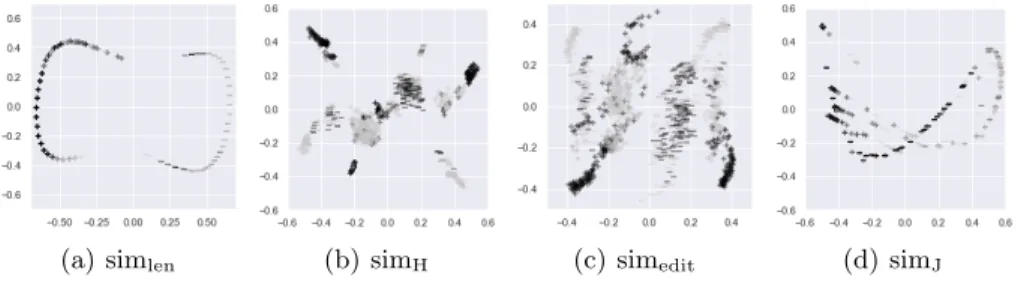
(a) simlen (b) simH (c) simedit (d) simJ
Fig. 1. t-SNE-based scatter plots for the considered similarity measures. Positive and negative formulas are marked using + and −, respectively, using a gray shade reflecting ARI (dark shades for low ARI and vice versa.)
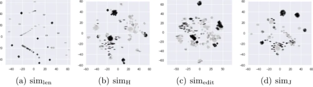
(a) simlen (b) simH (c) simedit (d) simJ
Fig. 2. PCA-based scatter plots. Same notations as in Figure 1.
sures detailed below. The result of this mapping is considered as an intermediate representation to be further processed as explained in the rest of the paper. Length-based similarity This similarity is obtained by comparing the textual representation length of two formulas φ1 and φ2 as follows:
slen(φ1, φ2) = 1 −
|#φ1− #φ2|
max{#φ1, #φ2}
, (1)
where #φ denotes the length of the textual representation of φ. Normalization is required in order to transform the distance |#φ1− #φ2| into a similarity.5
Such measure, however, cannot be reasonably expected to be able to capture meaningful information, as it merely relies on string length. For instance, two formulas whose formal description have equal length will always exhibit maximal similarity, regardless of the concepts they express. Nonetheless, such similarity has been included as a sort of litmus test. Anyhow, (1) is excessively naive, for it would assign quasi-maximal similarity to a formula and its logical negation: indeed, their descriptions would differ only for a trailing minus character. This inconvenience can be easily fixed by complementing to 1 the above definition
5
The used implementations of t-SNE and PCA in scikit-learn [16] accept, respectively, a distance and a similarity matrix. Thus we normalized all similarities.
(a) simlen (b) simH (c) simedit (d) simJ
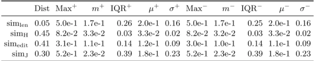
Fig. 3. Scatter plots of the output of PCA, followed by t-SNE. Same notations as in Figure 1.
when the signs of the two formulas are opposed and limiting the comparison to the base axiom only:
simlen(φ1, φ2) =
(
1 − slen(abs(φ1), abs(φ2)) if sgn(φ1) 6= sgn(φ2),
slen(φ1, φ2) otherwise.
(2)
This basically ensures, as one would intuitively expect, that the similarity be-tween a formula and its negation be zero.
Hamming similarity Despite its simplicity, length-based similarity catches very simple instances of syntactical similarities (e.g. when identical—or almost identi-cal—formulas only differ from synonymous class names); in this respect, it is reasonable to obtain better results if the distance is defined in a smarter way. This can be achieved for instance considering simH(φ1, φ2) = H(abs(φ1), abs(φ2)), if
sgn(φ1) 6= sgn(φ2), 1 − H(φ1, φ2) otherwise, where H is the normalized Hamming
distance between the textual representations of two formulas, that is the fraction of positions where such strings contain a different character, aligning them on the left and ignoring the extra characters of the longest string.
Levenshtein similarity We can aim at grasping more sophisticated forms of syntactical similarities, and even simple semantic similarities. To such extent, we considered simedit(φ1, φ2) = Lev(abs(φ1), abs(φ2)) if sgn(φ1) 6= sgn(φ2),
1 − Lev(φ1, φ2) otherwise, where Lev is the normalized Levenshtein distance [8]
between strings representing two formulas, intended as the smallest number of atomic operations allowing to transform one string into the other one.
Jaccard similarity Semantics heavily depends on context. This is why we also consider the similarity measure introduced in [11] exploiting notation of Sect. 1:
simJ(φ1, φ2) =
k[A] ∩ [B] ∪ [C] ∩ [D]k
k[A] ∪ [C]k , (3)
where φ1 is the subsumption A v B, and φ2is C v D. Note that among all the
Table 1. Radius statistics for PCA-based clusters. Rows: similarity measures; Dist: average Euclidean distance between postivie and negative clusters; Max, m, IQR, µ, and σ: maximum, median, interquartile range, mean, and standard deviation for cluster radius. Indices are computed separately for positive and negative formulas and shown columns marked with + and −.
Dist Max+ m+ IQR+ µ+ σ+ Max− m− IQR− µ− σ− simlen 0.05 5.0e-1 1.7e-1 0.26 2.0e-1 0.16 5.0e-1 1.7e-1 0.25 2.0e-1 0.16
simH 0.45 8.2e-2 3.3e-2 0.03 3.3e-2 0.02 8.2e-2 3.2e-2 0.03 3.3e-2 0.02
simedit 0.41 3.1e-1 1.1e-1 0.14 1.2e-1 0.09 3.0e-1 1.0e-1 0.14 1.1e-1 0.09
simJ 0.30 5.2e-1 2.3e-2 0.39 1.8e-1 0.23 5.2e-1 2.3e-2 0.39 1.8e-1 0.23
form of the formulas (subsumptions) and their meaning within a dataset. It has been termed Jaccard similarity because (3) racalls the Jaccard similarity index. Figures 1 and 2 show the obtained set of points in R2when applying t-SNE and kernel PCA, coupled with the above similarities, to the considered subsump-tion formulas6. In each plot, + and − denote the images of positive and negative formulas in R2through the reduction technique; the color of each bullet reflects
the ARI associated to a formula (cf. Sect. 2), with minimal and maximal values being mapped onto dark and light gray. Figure 3 shows the same scatter plots when PCA and t-SNE are applied in chain, as commonly advised [9]. In partic-ular, not having here an explicit dimension for the original space of formulas, we extracted 300 principal components via PCA and considered the cumulative fraction of explained variance (EV) for each of the extracted components, after the latter were sorted by nondecreasing EV value. In such cases, the number of components to be considered is the one explaining a fixed fraction of the total variance, and we set such fraction to 75%, which led us to roughly 150 components, to be further reduced onto R2via t-SNE.
Recalling that our final aim is to tell “good” formulas from “bad” ones, where “good” means a high ARI, i.e., light gray symbols in the scatter plots, the obtained results highlight the following facts.
– In all simlen plots, light and dark bullets tend to heavily overlap, thus
con-firming that simlen is not a suitable choice for our classification purposes.
– A similar behavior is generally exhibited by PCA; however, shapes in Fig-ures 2(a) and 2(d) strongly recall the projection onto R2 of a saddle-shaped
manifold, thus suggesting a low-dimensional intrinsic dimensionality. Leaving apart the length-based similarity and the sole kernel PCA technique, we are left with six possibilities, which are hard to rank via qualitative judgment only. We can only remark that simHtends to generate plots where the two classes
do not appear as sharply distinguished as in the remaining cases. However, this criterion is too weak and, therefore, a quantitative approach is needed. This is
6
Code and data to replicate all experiments described in the paper is available at https://github.com/dariomalchiodi/MDAI2020.
Table 2. Radius statistics for clusters of points obtained through t-SNE. Same nota-tions as in Table 1.
Dist Max+ m+ IQR+ µ+ σ+ Max− m− IQR− µ− σ− simlen 15.80 7.8e+1 3.4e+1 36.62 3.4e+1 23.12 8.0e+1 3.7e+1 37.35 3.6e+1 24.01
simH 60.29 1.2e+1 3.0e+0 7.10 4.4e+0 3.98 1.0e+1 2.1e+0 5.26 3.4e+0 3.23
simedit 57.66 2.7e+1 8.3e+0 11.42 9.6e+0 7.62 2.6e+1 7.6e+0 9.31 8.9e+0 6.96
simJ 2.33 3.8e+0 9.1e-1 2.75 1.5e+0 1.44 3.3e+0 6.3e-1 2.54 1.3e+0 1.33
Table 3. Radius statistics for clusters of points obtained chaining kernel PCA and t-SNE. Same notations as in Table 1.
Dist Max+ m+ IQR+ µ+ σ+ Max− m− IQR− µ− σ− simlen 17.76 7.9e+1 3.5e+1 36.68 3.5e+1 3.65 8.0e+1 3.7e+1 37.87 3.7e+1 24.45
simH 56.19 3.3e+0 1.1e+0 1.51 1.3e+0 0.91 3.1e+0 1.1e+0 1.41 1.2e+0 0.87
simedit 60.56 3.1e+1 1.0e+1 14.28 1.2e+1 9.22 3.2e+1 1.1e+1 13.97 1.2e+1 9.45
simJ 13.02 2.3e+1 1.3e+0 16.47 7.8e+0 9.72 2.6e+1 1.4e+0 16.46 7.9e+0 10.05
why we considered the radius statistics of the clusters of points in R2 referring
to a same concept. More precisely:
– each concept is identified by an OWL class (such as for instance Coach, TennisLeague, Eukaryote, and so on);
– given a concept, we identify all positive formulas having it as antecedent,7
and consider the positive cluster of corresponding points in R2; we proceed
analogously for the negative cluster ;
– we subsequently obtain the centroids of the two clusters and compute their Euclidean distance; moreover, we consider the population of distances be-tween each point in a cluster and the corresponding centroid. Such popu-lation is described in terms of basic descriptive indices (namely, maximum, mean and standard deviation, median and interquartile range (IQR)). Thus, for each combination of reduction technique, similarity measure, and con-cept, we obtain a set of measurements. In order to reduce this information to a manageable size, we average all indices across concepts: Tables 1–3 summarize the results, for which we propose the following interpretation:
– the use of kernel PCA results in loosely decoupled clusters: indeed, indepen-dently of the considered similarity measure, the distance between positive and negative formulas is generally smaller than the sum of the radii of the corresponding clusters (identified with the max index); moreover, all mea-sured indices tend to take up similar values;
– as already found out in the qualitative analysis of Figures 1–3, a weakness analogous to that illustrated in the previous point tends to be associated to simlen, regardless of the chosen reduction technique;
7
We also repeated all experiments considering both antecedents and consequents, obtaining comparable results.
– quite suprisingly, simHis the only similarity measure which results in sharply
distinguished clusters when coupled with t-SNE.
4
Learning ARI
As all considered formulas have been mapped to points in a Euclidean space, it is now easy to use the images of the considered mappings as patterns to be fed to a supervised learning algorithm, whose labels are the ARI of the relevant formulas. More precisely, we considered the following models (and, specifically, their implementation in scikit-learn [16]), each described together with the hy-perparameters involved in the model selection phase:
– Decision trees (DT), parameterized on purity index, maximal number of leaves, maximal number of features, and maximal tree depth;
– Random forests (RF), parameterized on the number of trees, as well as on the same quantities as DT;
– Naive Bayes with Gaussian priors (NB), without hyperparameters; – Linear Discrimimant Analysis (LDA), without hyperparameters;
– Three-layered feed-forward neural networks (NN), parameterized on the num-ber of hidden neurons;
– Support vector classifiers (SVC), parameterized on the tradeoff constant and on the used kernel.
When applicable, model selection was carried out via a repeated holdout con-sisting of five iterations, each processing a grid of the above-mentioned values for hyperparameters, shuffling available data, and considering a split assigning 80%, 10%, and 10% of points, respectively, to train, validation, and test. When model selection was not involved, respectively 80% and 20% of the available examples where assigned to training and test.
In order to build examples to be fed to learning algorithms, each formula needed to be associated with a binary label. That was done through binarization of the ARI values, using a threshold α ∈ {i/10 for i = 1, . . . , 9}. More precisely, an experiment was carried out for each of the possible thresholding levels. Finally, the transformation of formulas into vectors was done by considering different values for the dimension d of the resulting Euclidean space, namely the values in {2, 3, 5, 10, 30} were tested. Summing up, for each reduction technique R (that is, either PCA or t-SNE coupled with any similarity measure) and considered dimension d, the following holdout protocol was iterated ten times:
1. R was applied to the available data in order to obtain a set of vectors in Rd;
2. for each model M such vectors were randomly shuffled and subsequently divided into training, validation (if needed), and test set;
3. for each threshold value α, a model selection for M using the data in train-ing and validation set was carried out, testtrain-ing the selected model against generalization using the test set;
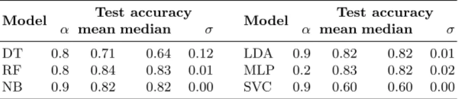
Table 4. Test set accuracy for the considered learning algorithms, when fed with points in R2 representing the original formulas transformed through kernel PCA using sim
J.
Model Test accuracy Model Test accuracy α mean median σ α mean median σ DT 0.8 0.71 0.64 0.12 LDA 0.9 0.82 0.82 0.01 RF 0.8 0.84 0.83 0.01 MLP 0.2 0.83 0.82 0.02 NB 0.9 0.82 0.82 0.00 SVC 0.9 0.60 0.60 0.00 Table 5. Comparison between test set median accuracy of algorithms using PCA. Rows: models; columns: similarity; d: space dimension.
d = 2 d = 3 d = 5 d = 10 H J edit H J edit H J edit H J edit DT 0.62 0.64 0.68 0.62 0.60 0.66 0.62 0.60 0.66 0.62 0.64 0.66 RF 0.67 0.83 0.67 0.66 0.81 0.70 0.66 0.82 0.68 0.64 0.81 0.68 NB 0.62 0.82 0.69 0.63 0.80 0.68 0.63 0.83 0.68 0.62 0.81 0.68 LDA 0.52 0.82 0.68 0.52 0.82 0.67 0.52 0.83 0.68 0.53 0.83 0.68 MLP 0.62 0.82 0.66 0.61 0.83 0.68 0.63 0.80 0.68 0.61 0.82 0.68 SVC 0.60 0.60 0.60 0.60 0.60 0.60 0.60 0.60 0.60 0.60 0.60 0.60
Table 6. Comparison between algorithms using t-SNE. Same notations as in Table 5. d = 2 d = 3 d = 5 d = 10
H J edit H J edit H J edit H J edit DT 0.66 0.62 0.62 0.65 0.62 0.60 0.65 0.62 0.60 0.67 0.61 0.60 RF 0.64 0.66 0.65 0.66 0.64 0.66 0.65 0.63 0.65 0.66 0.66 0.66 NB 0.69 0.65 0.63 0.69 0.66 0.64 0.65 0.65 0.65 0.67 0.65 0.62 LDA 0.67 0.65 0.62 0.68 0.68 0.62 0.68 0.67 0.62 0.70 0.68 0.62 MLP 0.70 0.66 0.63 0.68 0.60 0.61 0.64 0.57 0.61 0.68 0.58 0.60 SVC 0.60 0.60 0.60 0.60 0.60 0.60 0.60 0.60 0.60 0.60 0.60 0.60
Table 4 shows the results obtained when using kernel PCA with Jaccard simi-larity. For each model, the optimal value of α is shown, as well as the estimated generalization capability, in terms of mean and median accuracy on the test set. Tables 5 and 6 show a more compact representation of the corresponding results when considering the possible combinations of learning algorithm, sim-ilarity measure, reduction technique, and dimension of the space onto which formulas are mapped. Because, as expected, the length-based distance always gave the worst results, it has been omitted from the tables to save space. The same applies to the results obtained when setting d = 30, which in this case did not give any significant improvement w.r.t. the figures for d = 10.
Looking at these results, it is immediately clear that SVC is systematically outperformed by the remaining models, and the results it obtains are indepen-dent of the combination of reduction technique, similarity measure, and space
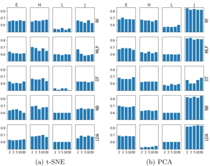
(a) t-SNE (b) PCA
Fig. 4. Comparison of the more significative results in learning ARI when using t-SNE (a) and PCA (b). Rows are associated to learning algorithms, using the abbreviations introduced in Sect. 4, while columns refer to similarity measures (E: simedit, H: simH,
L: simlen, J: simJ). Each graph plots test set accuracy vs. number of dimensions.
dimension. Moreover, the best results (highlighted using boldface in the tables) are almost always higher when using kernel PCA, thus somehow in contrast with the preliminary results obtained in Sect. 3. In order to further analyze this trend, Figure 4 graphically shows a subset of the obtained results, where SVC is left out. The graphs highlight that the space dimension d has a weak influence on the results, and that simlenalways attains a low score, thus it has been excluded
from the rest of the analysis. Experiments can be divided into three groups: – all combinations of LDA with simH, getting a bottom-line performance,
– a majority of cases where median accuracy lays roughly between 60 and 70%, notably containing all remaining results based on t-SNE, and
– a top set of experiments with median accuracy > 80%, including all those involving kernel PCA with simJ and any learning algorithm but DT.
In order to verify that there is a significant difference between the experi-ments in these groups, we executed the Cram´er-Von Mises (CVM) test [2]. For the sake of conciseness, we will call a case any combination of learning algorithm, dimensionality reduction technique, dimension of the resulting space, and simi-larity measure (excluding, as previously stated, SVC and simlen). For each case,
we repeated the experiments ten times, thus getting a sample of ten values for the median test set error. We then gathered cases in the following categories:
GtopPCA, Gmid PCA, G
btm
PCA: respectively the best, middle, and low performing cases
using PCA (corresponding to the three items in the previous list); GtSNE: all
cases using tSNE, i.e. those shown in Figure 4(a). Now, given a generic pair of cases taken from GtopPCA and Gmid
PCA, the hypothesis that the corresponding test
error samples are drawn from the same distribution is strongly rejected by the CVM test, with p < 0.01. The same happens when considering any other pair of groups related to PCA, and these results do not change if Gmid
PCAis swapped with
GtSNE. On the other hand, the same test run on two cases from GtopPCA didn’t
reject the same hypothesis in 81% of the times.
5
Conclusions
Our results show that it is possible to learn reasonably accurate predictors of the score of candidate axioms without having to resort to sophisticated (and expensive-to-compute) semantics-based similarity measures. Indeed, we showed that using a dimensionality-reduction technique to map candidate axioms to a low-dimension space allows supervised learning algorithms to effectively train predictive models of the axiom score. This agrees with the observation that there are no obvious indicators to inform the decision to choose between a cheap or expensive similarity measure based on the properties of an ontology [1].
Our findings can contribute to dramatically speed up ontology-learning ap-proaches based on exhaustive or stochastic generate-and-test strategies, like [3, 12]. As a further development, we plan to apply to the same dataset more sophis-ticated techniques able to learn the ARI without the need of binarizing labels.
Acknowledgments
Part of this work was done while D. Malchiodi was visiting scientist at Inria Sophia-Antipolis/I3S CNRS Universit´e Cˆote d’Azur. This work has been sup-ported by the French government, through the 3IA Cˆote dAzur “Investments in the Future” project of the Nat’l Research Agency, ref. no. ANR-19-P3IA-0002.
References
1. Alsubait, T., Parsia, B., Sattler, U.: Measuring conceptual similarity in ontologies: How bad is a cheap measure? In: Description Logics. pp. 365–377
2. Anderson, T.W.: On the distribution of the two-sample cramer-von mises criterion. The Annals of Mathematical Statistics 33(3), 1148–1159 (1962)
3. B¨uhmann, L., Lehmann, J.: Universal OWL axiom enrichment for large knowledge bases. In: EKAW 2012. pp. 57–71
4. Dubois, D., Prade, H.: Possibility Theory—An Approach to Computerized Pro-cessing of Uncertainty. Plenum Press, New York (1988)
5. Fleischhacker, D., V¨olker, J., Stuckenschmidt, H.: Mining RDF data for property axioms. In: OTM 2012. pp. 718–735
6. Huitzil, I., Straccia, U., D´ıaz-Rodr´ıguez, N., Bobillo, F.: Datil: Learning fuzzy ontology datatypes. In: IPMU 2018. pp. 100–112
7. Lehmann, J., V¨olker, J. (eds.): Perspectives on Ontology Learning, Studies on the Semantic Web, vol. 18. IOS Press, Amsterdam (2014)
8. Levenshtein, V.I.: Binary codes capable of correcting deletions, insertions, and reversals. Soviet Physics Doklady 10(8), 707–710 (February 1966)
9. Maaten, L.v.d., Hinton, G.: Visualizing data using t-sne. Journal of machine learn-ing research 9(Nov), 2579–2605 (2008)
10. Maedche, A., Staab, S.: Ontology learning for the semantic web. IEEE Intelligent Systems 16(2), 72–79 (2001)
11. Malchiodi, D., Tettamanzi, A.G.B.: Predicting the possibilistic score of owl axioms through modified support vector clustering. In: SAC 2018. pp. 1984–1991 12. Nguyen, T.H., Tettamanzi, A.: Learning class disjointness axioms using
grammat-ical evolution. In: EuroGP. pp. 278–294
13. Nonato, L.G., Aupetit, M.: Multidimensional projection for visual analytics: Link-ing techniques with distortions, tasks, and layout enrichment. IEEE Transactions on Visualization and Computer Graphics 25(8), 2650–2673 (2018)
14. Parsia, B., Motik, B., Patel-Schneider, P.: OWL 2 web ontology lan-guage structural specification and functional-style syntax (second edition). W3C recommendation, W3C (December 2012), http://www.w3.org/TR/2012/ REC-owl2-syntax-20121211/
15. Pearson, K.: LIII. on lines and planes of closest fit to systems of points in space. The London, Edinburgh, and Dublin Philosophical Magazine and Journal of Science 2(11), 559–572 (1901)
16. Pedregosa, F., Varoquaux, G., Gramfort, A., Michel, V., Thirion, B., Grisel, O., Blondel, M., Prettenhofer, P., Weiss, R., Dubourg, V., Vanderplas, J., Passos, A., Cournapeau, D., Brucher, M., Perrot, M., Duchesnay, E.: Scikit-learn: Machine learning in Python. Journal of Machine Learning Research 12, 2825–2830 (2011) 17. Sacha, D., Zhang, L., Sedlmair, M., Lee, J.A., Peltonen, J., Weiskopf, D., North,
S.C., Keim, D.A.: Visual interaction with dimensionality reduction: A structured literature analysis. IEEE transactions on visualization and computer graphics 23(1), 241–250 (2016)
18. Sch¨olkopf, B., Smola, A.J., M¨uller, K.: Kernel principal component analysis. In: International Conference on Artificial Neural Networks (ICANN). pp. 583–588 19. Straccia, U., Mucci, M.: pFOIL-DL: Learning (fuzzy) EL concept descriptions from
crisp OWL data using a probabilistic ensemble estimation. In: SAC 2015. pp. 345– 352
20. Stuckenschmidt, H.: Partial matchmaking using approximate subsumption. In: Proceedings of the Twenty-Second AAAI Conference on Artificial Intelligence, July 22-26, 2007, Vancouver, British Columbia, Canada. pp. 1459–1464
21. Tettamanzi, A.G.B., Faron-Zucker, C., Gandon, F.: Dynamically time-capped pos-sibilistic testing of subclassof axioms against rdf data to enrich schemas. In: K-CAP 2015. p. Article No.: 7
22. Tettamanzi, A.G.B., Faron-Zucker, C., Gandon, F.: Possibilistic testing of OWL axioms against RDF data. International Journal of Approximate Reasoning 91, 114–130 (December 2017)
23. Tettamanzi, A.G.B., Faron-Zucker, C., Gandon, F.L.: Testing OWL axioms against RDF facts: A possibilistic approach. In: EKAW 2014. pp. 519–530
24. T¨opper, G., Knuth, M., Sack, H.: Dbpedia ontology enrichment for inconsistency detection. In: I-SEMANTICS. pp. 33–40
25. Yin, H.: Nonlinear dimensionality reduction and data visualization: a review. In-ternational Journal of Automation and Computing 4(3), 294–303 (2007)