Fast balanced sampling for highly stratified population

Keywords:

Balanced sampling Stratified sampling Cube method

Unequal probability sampling Auxiliary information

a b s t r a c t

Balanced sampling is a very efficient sampling design when the variable of interest is cor-related to the auxiliary variables on which the sample is balanced. A procedure to select balanced samples in a stratified population has previously been proposed. Unfortunately, this procedure becomes very slow as the number of strata increases and it even fails to se-lect samples for some large numbers of strata. A new algorithm to sese-lect balanced samples in a stratified population is proposed. This new procedure is much faster than the existing one when the number of strata is large. Furthermore, this new procedure makes it possible to select samples for some large numbers of strata, which was impossible with the existing method. Balanced sampling can then be applied on a highly stratified population when only a few units are selected in each stratum. Finally, this algorithm turns out to be valuable for many applications as, for instance, for the handling of nonresponse.

1. Introduction

Auxiliary information is a central point in survey statistics. It is widely used in a large set of sampling designs. For instance, auxiliary information can be used to select stratified samples; it can also be used to define sampling designs with unequal probabilities. Regardless of the way auxiliary information is used, the main goal is to improve the quality of the estimates.

A stratified sampling design consists of dividing the population into subgroups (the strata) and of selecting samples in each stratum. Auxiliary information must be available to define the strata. The way the population has to be stratified is _{not always clear. A lot of research has been conducted on this topic. Neyman (1934) looked into optimum allocation. A} method for the iterative improvement of the points of stratification was given and illustrated in Dalenius and Hodges (1959). Bülher and Deutler (1975) presented a method to determine a global optimal solution by linear programming whereas Lavallée _{and Hidiroglou (1988) tackled the issue of stratification of a highly skewed population. Díaz-García and} Garay-Tápia (2007) considered the allocation problem in stratified surveys as a problem of stochastic programming. Stratified sampling designs have the interesting property of reducing the variance of the Horvitz–Thompson estimator compared to unstratified _{sampling designs if the values of the variable of interest are somewhat homogeneous inside the strata.}

A balanced sampling design consists of selecting samples in such a way that the Horvitz–Thompson estimator for some auxiliary variables matches the population total. These auxiliary variables are called the balancing variables. Deville et al. (1988) described a method to obtain balanced samples and, later, the cube method (Deville and Tillé, 2004) was proposed for the same purpose. Some methods have been proposed for the computing of optimal inclusion probabilities for balanced sam-pling _{as for instance those given in Tillé and Favre (2005), Nedyalkova and Tillé (2008), and Chauvet et al. (2011a). A balanced} sampling design is a very efficient sampling design when the variable of interest is correlated to the balancing variables.

In the presence of auxiliary variables correlated to the variable of interest and in the presence of strata, it is thus very useful to select samples applying a procedure which produces both stratified and balanced samples. Brewer (1999), indeed,

Published in Computational Statistics and Data Analysis 74, 81-94, 2014 which should be used for any reference to this work

Fast

balanced sampling for highly stratified population

Caren

Hasler, Yves Tillé

∗

showed that balanced sampling inside the strata can considerably improve the robustness and efficiency of some estimates.

Chauvet(2009) proposed a stratified balanced sampling procedure: his algorithm selects samples which are approximately balanced in each stratum, balanced across the entire population and such that the sample size is fixed in each stratum. Un-fortunately, Chauvet’s procedure can be slow when the number of strata is large. In this paper, a new algorithm for stratified balanced sampling is proposed. This algorithm is much faster than Chauvet’s algorithm when the number of strata is large. The proposed algorithm turns out to be valuable for many applications, namely the selection of balanced samples in highly stratified populations when only a few units are selected in each stratum. For example, the proposed algorithm could improve the quality of estimates produced by some large-scale surveys. Indeed, in some large-scale multistage surveys, only one or two primary sampling units or first-stage units are selected in each stratum and the number of strata can be very large. Besides, the proposed method can also be used to treat nonresponse. Stratified sampling has long been used for the purpose of imputation. For instance,Kalton and Kish(1984) had already proposed selecting stratified sample of respondents to act as donors in order to reduce imputation variance. This idea can be extended by using the proposed method for stratified balanced sampling. Indeed,Chauvet et al.(2011b) proposed a class of imputation methods that they called balanced random imputation and which use balanced sampling. This class of method is constructed such that the imputation variance is eliminated. Furthermore, the imputed values can be obtained through stratified balanced sampling. In this framework, however, the considered number of strata may be very large, hence the proposed method for stratified balanced sampling turns out to be useful in this context.

The paper is organized as follows. In Section2, notions and concepts of balanced sampling are reviewed. Then in Section3, Chauvet’s method is described. The new method is presented in Section4. A solution to apply the new method in cases where the sum of the inclusion probabilities is not an integer in each stratum is given in Section5. Section6focusses on estimation of the variance of the Horvitz–Thompson estimator whereas Section7presents a possible application of the new method to the handling of nonresponse. Brief simulation studies were conducted to test the performance of the new sampling algorithm, to test the accuracy of the proposed formulas for the variance, and to illustrate the application of the new sampling algorithm in the context of handling of nonresponse. The results of these studies are given in Section8. Finally, Section9closes the paper with concluding remarks.

2. Balanced sampling

Consider a finite population U

= {1

, . . . ,

k

, . . . ,

N}of size N in which the aim is to select a random sample S, i.e. a subset of the population randomly selected. A sampling design p

(·)

assigns to each subset s

⊂

U a probability p

(

s

)

of being selected with



s⊂U

p

(

s

) =

1

.

The inclusion probability

π

kis the probability of selecting a particular unit k. The aim is to estimate a total

ty

=



k∈U

yk

,

for some variable of interest y. If

π

k

>

0 for all k

∈

U, then theHorvitz and Thompson(1952) estimator given by



ty

=



k∈S yk

π

k

,

is unbiased for ty.

Consider now that a column vector xk

∈

Rqof auxiliary variables is available for all the units k

∈

U. A sampling design p

(·)

with inclusion probabilities

π

kis said to be balanced on xkif



k∈s xk

π

k

=



k∈U xk

,

(1)

for every subset s

⊂

U such that p

(

s

) >

0. In many cases, it is not possible to find a subset s

⊂

U satisfying exactly Eq.(1). As a result, a sampling design p

(·)

can often not be exactly balanced. This problem is referred to as a rounding problem. Consider the sample membership indicators s

=

(

s1

. . .

sk

. . .

sN

)

⊤where

sk

=



1 if k

∈

S

,

0 if k

̸∈

S

.

When a rounding problem is encountered, it is not possible to find a vector s of zeros and ones that exactly satisfies the equation



k∈U xk

π

k sk

=



k∈U xk

.

Deville and Tillé(2004) proposed the cube method, which allows for the selection of balanced samples. The cube method is an algorithm composed of two phases: the flight phase and the landing phase. In what follows, the results given by the two phases of the algorithm are presented. The aim is not to describe the cube method in detail but only the outputs of both phases.

•

The flight phase provides a vector of random variables

φ = (φ

1

. . . φ

k

. . . φ

N

)

⊤, with 0

≤

φ

k

≤

1, such that

(i) E

(φ

k

) = π

kfor all k

∈

U,

(ii)



k∈U xk πk

φ

k

=



k∈Uxk,

(iii) #{k|0

< φ

k

<

1} ≤q, where q is the dimension of xk.

A unit k with

φ

k

=

1 is selected in the sample and a unit k with

φ

k

=

0 is definitely rejected. Whether there is a rounding

problem or not, the equation in (ii) is exactly satisfied. In the presence of a rounding problem and as explained at the end of the previous paragraph, it is, however, not possible to find a vector

φ

of zeros and ones which is a solution to the equation in (ii). In that case, some

φ

k’s are not integers and some units are not yet selected or rejected at the end of the

flight phase. It is possible to show, as stated in (iii), that the number of non-integer

φ

k’s is at most q. In other words, at most

q units are not yet selected or rejected at the end of the flight phase.Chauvet and Tillé(2006) proposed a fast algorithm for the flight phase. In what follows, the flight phases are carried out by means of this algorithm.

•

The landing phase is used to deal with the rounding problem. Its main idea is to relax the balancing constraint in order to address the problem of the units that have not yet been rejected or selected at the end of the flight phase. The landing phase provides a vector s

=

(

s1

. . .

sk

. . .

sN

)

⊤of sample membership indicator such that

(i) E

(

s_k

|

φ) = φ

_kfor all k

∈

U, (ii)



k∈U xk πksk

≈



k∈Uxk.

A unit k with sk

=

1 is selected in the sample and a unit k with sk

=

0 is rejected. At the end of the landing phase, every

unit has been selected or rejected.Deville and Tillé(2004) have proposed two ways of running the landing phase: by linear programming or by suppression of variables. The landing phase by linear programming consists of solving a linear pro-gramming problem through the simplex algorithm. The list of all possible samples from a population of size q, where q is the dimension of xk, must be generated and this can be impossible when q exceeds a limit. Therefore, the landing phase by

linear programming cannot be applied when the number of auxiliary variables q exceeds this limit, which is generally 20. When one of the variables in xkis equal or proportional to

π

k, the balancing constraint(1)implies that



k∈s

π

k

π

k

=



k∈U

π

k

⇔

n

(

s

) =



k∈U

π

k

,

where n

(

s

)

is the size of the subset s

⊂

U. This means that the sampling design has a fixed sample size. This equality can only be exactly satisfied if the sum of the inclusion probabilities is an integer. If the sum of the inclusion probabilities is not an integer, then the cube method usually selects a sample whose size is the smallest integer larger than this sum or the largest integer smaller than this sum.

3. Chauvet’s method for stratified balanced sampling

The population is presumed to be partitioned into H nonoverlapping strata U1

, . . . ,

Uh

, . . . ,

UH. Let

1

(

k

∈

Uh

)

be the

stratum membership indicator that takes value 1 if unit k belongs to stratum h and 0 otherwise. A stratified balanced sampling design p

(·)

is a sampling design which is balanced on xkin each stratum, i.e.



k∈s∩Uh xk

π

k

=



k∈Uh xk

,

for each s

⊂

U with p

(

s

) >

0 and for each h

=

1

, . . . ,

H.

Suppose that the goal is to balance on xk

∈

Rqsuch that none of the auxiliary variables is proportional to

π

k. Chauvet’s

method (Chauvet, 2009) is presented in Algorithm 1. The main idea of this method is to first run flight phases independently inside the strata. This ensures that the samples are as balanced as possible within the strata. Next, in a second step, a general flight phase is run on all the units of the population that have not yet been selected or rejected at the end of the first step. It results in samples that are as balanced as possible across the entire population. Finally, a third step is carried out to handle the case of units that have not yet been rejected or selected at the end of the second step. Originally inChauvet(2009), the third step consisted of unequal probability sampling whereas the third step of the new procedure presented in Section4

consists of a landing phase by suppression of variables. A landing phase by suppression of variables takes the balancing constraint into account and therefore provides more accurate estimates than unequal probability sampling. Henceforth, for a fair comparison between methods with respect to the accuracy of the estimates and as pointed out by one of the referees, the third step of Chauvet’s algorithm has here been modified onto a landing phase by suppression of variables.

In step 1 of Algorithm 1, q

+

1 balancing variables are considered in each flight phase. Therefore at most q

+

1 units in each stratum are not yet selected or rejected at the end of step 1. As a result, step 2 concerns at most

(

q

+

1

)

H units. In step 2, H

+

q balancing variables are considered in the flight phase. It may be impossible to carry out the flight phase of step 2 if the considered design is highly stratified (i.e. if H is very large). Indeed, the fast algorithm for the flight phase proposed byChauvet and Tillé(2006) requires the use of a matrix that is equal in size to the number of balancing variables times the number of balancing variables plus one. However, this approach can only be used with matrices of a limited size. This limit depends on the computer. If a highly stratified design is considered, the flight phase of step 2 requires the use of a huge matrix and it may be impossible to carry it out. Henceforth, Algorithm 1 is likely to fail for highly stratified designs.

Algorithm 1 Chauvet stratified balanced sampling with step 3 by landing phase by suppression of variables Step 1: Carry out a flight phase, with balancing variables

(π

k x⊤k

)

⊤

and inclusion probabilities

π

kindependently in each

stratum Uh.

Step 1 provides vector

φ

of

φ

k’s.

Step 2: Carry out a flight phase, with balancing variables



φ

k

1

(

k

∈

U1

) . . . φ

k

1

(

k

∈

Uh

) . . . φ

k

1

(

k

∈

UH

)

φ

kx⊤k

π

k



⊤

and inclusion probabilities

φ

kon the set of units with non-integer

φ

k, i.e. on the units that are not yet selected or

rejected at the end of step 1. Step 2 provides vector

ψ

of

ψ

k’s.

Step 3: Do a landing phase with inclusion probabilities

ψ

kand balancing variables



ψ

k

1

(

k

∈

U1

) . . . ψ

k

1

(

k

∈

Uh

) . . . ψ

k

1

(

k

∈

UH

)

ψ

kx⊤k

π

k



⊤

on the set of units with non-integer

ψ

k. Use the landing phase by suppression of variables.

4. New procedure for highly stratified balanced sampling

In this section, it is supposed that the sum of the inclusion probabilities in each stratum



k∈Uh

π

k

=

nh

,

is an integer. This hypothesis will be relaxed in Section5but will considerably simplify the complexity of the proposed algorithm. The main idea of the proposed method described in Algorithm 2, is to first run a flight phase independently in each stratum. Then, in a second step, U1and U2are merged and a flight phase is run. Next, U1and U2are merged with U3

and a flight phase is run again and so on. Finally, a landing phase by suppression of variables is carried out in a third step. Algorithm 2 New procedure for highly stratified balanced sampling

Step 1: Carry out a flight phase, with balancing variables

(π

k x⊤k

)

⊤

and inclusion probabilities

π

kindependently in each

stratum Uh.

Step 1 provides vector

φ

(1)of

φ

_k(1)’s. Step 2: For j

=

2 to H:

•

Carry out a flight phase on the union of strata U1

, . . . ,

Uj, with balancing variables

z(_kj)

=



φ

(j−1) k

1

(

k

∈

U1

) . . . φ

( j−1) k

1

(

k

∈

Uj

)

φ

(j−1) k x ⊤ k

π

k



⊤

and inclusion probabilities

φ

(_kj−1)on the set of units with non-integer

φ

_k(j−1). The flight phase provides a vector

φ

(j)_of

_φ

(j)

k ’s for units with non-integer

φ

(j−1)

k .

•

Set

φ

_k(j)

=

φ

_k(j−1)for units with integer

φ

_k(j−1). Step 2 provides vector

φ

(H)of

φ

_k(H)’s.

Step 3: Do a landing phase with inclusion probabilities

φ

_k(H)and balancing variables

z(_kH+1)

=



φ

(H) k

1

(

k

∈

U1

) . . . φ

k(H)

1

(

k

∈

UH

)

φ

(H) k x ⊤ k

π

k



⊤

on the set of units with non-integer

φ

_k(H). Use the landing phase by suppression of variables.

This alternative implementation might look like a simple variant but it actually offers major advantages. An important advantage is that it greatly reduces computation time when some large numbers of strata are considered. This reduction in computation time is explained in what follows. In step 2 of Algorithm 2, the flight phases are carried out with the balancing variables z(_kj). Consider matrix Z(j)_{whose rows are the z}(j)⊤

k restricted to the k with non-integer

φ

(j−1)

k , i.e. the k such that

Result. With Algorithm 2, for j

=

2

, . . . ,

H (i) #



k

∈



j i=1Ui







0

< φ

(j) k

<

1



≤

2q

+

2,

(ii) the number of non-null columns of matrix Z(j)_{is less than or equal to 2q+2, where a null column is a column that contains}

only zeros.

The proof is given in theAppendixand requires that the sum of the inclusion probabilities is an integer in each stratum. In light of this result, it appears that the flight phase must never be applied on a matrix of balancing variables with more than 2q

+

2 columns with Algorithm 2 because the null columns can be removed. However the flight phase could be applied on a matrix of balancing variables with up to q

+

H columns with Algorithm 1. This size difference of the matrices considered in the flight phases affects the execution time of the algorithms. Indeed, even if Algorithm 2 requires us to run 2H

−

1 flight phases against only H

+

1 for Algorithm 1, Algorithm 2 becomes much faster than Algorithm 1 as H increases. Even more interesting is the fact that Algorithm 2 is much more resistant to numerical instability than Algorithm 1 thanks to the reduction in size stated above. Indeed, numerical instability increases when the dimension of the matrices to deal with increases. In step 2 of Algorithm 1, flight phases operate with matrices of up to

(

q

+

H

) × (

q

+

H

+

1

)

in size whereas flight phases operate with matrices of up to

(

2q

+

2

) × (

2q

+

3

)

in size in step 2 of Algorithm 2. As this dimension depends on H for Algorithm 1, numerical instability increases as H increases. This is not the case with Algorithm 2.

Another advantage of the proposed method is that a landing phase can be applied in the last step even if the population is highly stratified. Indeed, at the last loop of step 2, we have

#{k

∈

U|0

< φ

_k(H)

<

1} ≤2q

+

2

.

This implies that the last step concerns at most 2q

+

2 units. This quantity is independent of the number of strata H. Consequently, a landing phase can be applied in step 3 regardless of the number of strata. Therefore, the balancing can be taken into consideration in step 3 of Algorithm 2 even if the population is highly stratified. As far as the last step of Algorithm 1 is concerned, a landing phase may not be applied for highly stratified populations as the number of units considered can reach q

+

H. The landing phase of step 3 of Algorithm 2 must be done by suppression of variables in order to ensure fixed size sampling inside the strata. Indeed, steps 1 and 2 of Algorithm 2 consist of flight phases. The balancing equations of the carried out flight phases imply that



k∈Uh

φ

(j) k

=

nh

,

for each j

=

1

, . . . ,

H and each h

=

1

, . . . ,

H. In particular, the following equation



k∈Uh

φ

(H)

k

=

nh

,

(2)

is satisfied for each h

=

1

, . . . ,

H. In step 3 of Algorithm 2, a landing phase is carried out. The aim is to derive a sample s of sk’s. The balancing equations linked to the first H balancing variables

φ

k(H)

1

(

k

∈

Uh

),

h

=

1

, . . . ,

H simplify to



k∈Uh sk

=



k∈Uh

φ

(H) k

,

(3)

for h

=

1

, . . . ,

H. Combining Eq.(2)together with Eq.(3)leads to



k∈Uh

sk

=

nh

,

(4)

for h

=

1

, . . . ,

H. As nhis in this section supposed to be an integer, Eq.(4)can always be satisfied; all that is required is

to select nhunits in each stratum Uh. The landing phase by suppression of variables consists of alternate dropping the last

balancing variables and running a flight phase again until the remaining constraints are exactly satisfied. As explained above, the constraints linked to the first balancing variables

φ

(_kH)

1

(

k

∈

Uh

),

h

=

1

, . . . ,

H, can always be satisfied. As the landing

phase is carried out by suppression of variables in step 3 of Algorithm 2, only the last q variables

φ

(H)

k x ⊤ k

π

k

are suppressed and fixed size sampling inside the strata is ensured.

Furthermore, the selected sample s

=

(

s1

. . .

sk

. . .

sN

)

⊤satisfies E

(

sk

) = π

k. To summarize, the sampling design

associated with Algorithm 2 is balanced, can be highly stratified and ensures fixed size sampling within the strata. Selection of samples with highly stratified designs becomes tractable with this new procedure.

Parallel computing can be used to slightly speed up both Algorithms 1 and 2. Firstly, it is conceivable to carry out the flight phases of steps 1 of both Algorithms in parallel. It is also possible to adapt step 2 of Algorithm 2 to use parallel computing. Indeed, even though it is impossible to roughly apply parallel computing as iterative procedures are involved, step 2 can be adapted for it as follows. The procedure proposed in step 2 of Algorithm 2 can be applied in parallel on non-overlapping groups of strata first. Then some of these groups can be gathered and the same procedure can be used, and so on.

Finally, Algorithms 1 and 2 can both be applied if the number of balancing variables q exceeds the size of a stratum. However, the balancing does not perform in such a stratum. Indeed, the random vector provided by the flight phase of step 1 in such a stratum match the initial inclusion probabilities. It means that none of the units of this stratum are selected or rejected yet at the end of the flight phase (except the one with integer inclusion probabilities). In steps 2, the same phenom-ena can occur, depending on whether the number of balancing variables still exceeds the number of units involved in the flight phases. Steps 3 can be applied if the number of balancing variables q exceeds the size of a stratum.

5. Case where the sum of the inclusion probabilities is not an integer in each stratum

As explained before, great advantages of Algorithm 2 can be gained from the fact that the sum of the inclusion probabil-ities is an integer in each stratum. However, most of the stratified designs used in practice can show a sum of the inclusion probabilities which is not an integer in each stratum. Stratification with proportional allocation and stratification with op-timal allocation are, among others, such designs. In what follows, a procedure to extend the use of Algorithm 2 to the case in which the sum of the inclusion probabilities is not an integer in each stratum is presented. It thus becomes possible to apply the new algorithm regardless of which stratified design is used.

The goal of this section is to introduce a procedure to round the sum of the inclusion probabilities in each stratum. This is a typical problem of rounding of allocations. This topic has already been widely explored and several procedures already exist such as those implemented in the R package stratification byBaillargeon and Rivest(2011) or those presented byWright

(2012). We propose a new random procedure of rounding that agrees with the balancing in the sense that it does not overly unbalance the totals of the auxiliary variables. Hence, the proposed rounding procedure consists of randomly rounding the sum of the inclusion probabilities in each stratum to the smallest integer larger than this sum or the largest integer smaller than this sum while taking into account constraints in relation to the balancing and sample size.

Let

⌊·⌋

denote the floor function. Consider nh

=



k∈Uh

π

k

,

and ph

=

nh

− ⌊n

h

⌋. We have 0

≤

ph

≤

1 for all h

=

1

, . . . ,

H. Since H



h=1 nh

=

n is an integer, m

=

H



h=1 ph is an integer as well.

The main idea of the proposed procedure is to select a sample of strata in which the number of selected units will be rounded up. Let J

=

(

J1

. . .

Jh

. . .

JH

)

denote a vector of sample membership indicators, where

Jh

=



1 if stratum Uhis selected in the sample of strata

,

0 otherwise

.

The probability that a stratum Uhis selected is ph, or equivalently E

(

Jh

) =

ph. The rounded sample size in strata h is then

n∗_h

= ⌊n

h

⌋ +

Jhfor h

=

1

, . . . ,

H. It means that the sample size in a stratum Uhis the smaller integer larger than nhif the

stratum is selected in the sample of strata and the larger integer smaller than nhif the stratum is not selected in the sample

of strata.

Constraints are imposed on the sample of strata J . First, it is selected such that the total number of selected units remains the same despite the change in sample size in some strata, i.e.

H



h=1 n∗_h

=

H



h=1 nh

.

This last equation is equivalent to

H



h=1

⌊n

h

⌋ +

Jh

=

H



h=1 nh

.

(5)

Moreover, as explained before, this rounding of the sample size must not overly unbalance the totals of the auxiliary variables, which is formalized as

H



h=1

⌊n

h

⌋ +

Jh nh



k∈Uh xk

=

H



h=1



k∈Uh xk

.

(6)

Considering Eq.(5)together with Eq.(6)leads to H



h=1

⌊n

h

⌋ +

Jh nh



k∈Uh



π

k xk



=

H



h=1



k∈Uh



π

k xk



,

or equivalently H



h=1 Jh nh



k∈Uh



π

k xk



=

H



h=1 ph nh



k∈Uh



π

k xk



.

The last equation can be rewritten

H



h=1 Jh ph V_h

=

H



h=1 V_h

,

(7) where Vh

=

ph nh



k∈Uh



π

k xk



=





ph ph nh



k∈Uh xk





.

Expression(7)is a usual system of balancing equations that can be solved by the cube method. The sample of strata J is therefore obtained by balanced sampling.

The inclusion probabilities

π

kmust then be slightly modified in new probabilities

π

k∗in such a way that



k∈Uh

π

∗ k

=

n ∗ h

= ⌊n

h

⌋ +

Jh

,

and that E

(π

∗

k

) = π

k. This modification is not trivial with unequal inclusion probabilities. Several solutions exist and are

discussed inGrafström et al.(2012). Once the new inclusion probabilities are computed, their sums are integers in the strata and Algorithm 2 can be used.

6. Variance estimation

The variance can be approximated with the method proposed byDeville and Tillé(2005). The same method was consid-ered inChauvet(2009). Set

zk

=



π

k

1

(

k

∈

U1

) π

k

1

(

k

∈

U2

) . . . π

k

1

(

k

∈

UH

)

x⊤k



⊤

.

An approximation of the variance of the total estimatortyis

varapp





ty

 =



k∈U bk



yk

π

k

−

β

⊤zk

π

k



2

,

(8) where bk

=

π

k

(

1

−

π

k

)

N N

−

(

H

+

q

)

and

β =





ℓ∈U b_ℓzℓ

π

ℓ z_ℓ⊤

π

ℓ



−1



ℓ∈U b_ℓzℓ

π

ℓ y_ℓ

π

ℓ

.

Various definitions of bk’s, and thus various approximations of the variance, are given inDeville and Tillé(2005). An

estima-tor of the approximated variance(8)is



var





ty

 =



k∈S ck



yk

π

k

− 

β

⊤zk

π

k



2

,

(9) where ck

=

(

1

−

π

k

)

n n

−

(

H

+

q

)

and



β =





ℓ∈S c_ℓzℓ

π

ℓ z_ℓ⊤

π

ℓ



−1



ℓ∈S c_ℓzℓ

π

ℓ y_ℓ

π

ℓ

.

The performance of the approximated variance and that of the variance estimator provided above are tested in Section8. Nevertheless, the variance estimator(9)is intractable if the number of balancing variables exceeds the sample size, which means here if H

+

q

>

n. Indeed, the matrix



ℓ∈Scℓzℓ_πℓzℓ ⊤

πℓ is in this case not invertible. However, it is possible in this case to

estimate the variance using a collapsed stratum procedure (seeWolter, 1985, pp. 50–57). Hence, the H strata are combined into G groups such that G

+

q

≤

n and the procedure given above to estimate the variance is applied considering the G groups instead of the H strata.

7. Illustration of the handling of nonresponse 7.1. Nonresponse and imputation

Imputation is a process that consists of replacing a missing value with a substituted one. It is especially used to compen-sate for item nonresponse. Imputation methods can be classified into two groups: deterministic and random. Deterministic methods are adequate for the purpose of totals estimation but they often fail to estimate quantiles because they disturb the distribution of the imputed variable. Random methods, on the other hand, are often appropriate for the aim of totals and quantiles estimation as they tend to preserve the distribution of the imputed variable. Unfortunately, the randomness of the imputation adds an additional amount of variance to the estimators. This additional amount of variance is called imputation variance. Random imputation methods that produce the least possible imputation variance are therefore effective methods of handling item nonresponse when the aim is to estimate totals as well as quantiles. Random hot-deck imputation is the process that consists of replacing a missing value with an observed value extracted from the same survey and selected at random.

7.2. Notation

A finite population U

= {

1

, . . . ,

k

, . . . ,

N

}

of size N is considered. In a first phase, a random sample S of size n is drawn with a given sampling design p

(·)

. For each k

∈

U, consider the first order inclusion probability

π

k

=

Pr

(

k

∈

S

)

and let

dk

=

1

/π

kdenote its Horvitz–Thompson weight (Horvitz and Thompson, 1952). It is supposed in this part that the vector

of q auxiliary variables xkis observed for each sampled unit k

∈

S. However, the values of the variable of interest ykare

potentially missing for some k

∈

S. Nonresponse can be viewed as a second phase of the sampling process. A subset Sr

⊂

S

of units k with observed ykis indeed obtained from S with a usually unknown conditional distribution q

(

Sr

|S

)

. Let Smdenote

the complement of Srin S, i.e. the subset of S containing the units k with missing yk(the nonrespondents). For k

∈

S, let rk

be the response indicator variable rk

=



1 if k

∈

Sr

,

0 otherwise

.

Imputation can be viewed as a third phase of the sampling process. Imputed values y∗_k

,

k

∈

Sm, are indeed drawn with a

conditional distribution I



y∗_k

|S

,

Sr



.

Suppose the aim is to estimate the regression coefficient

θ

N

=





k∈U xkx⊤k



−1



k∈U xkyk

.

In the case of complete response, the estimator



θ

N

=





k∈S dkxkx⊤k



−1



k∈S dkxkyk

,

is adequate. In the presence of nonresponse, this estimator is intractable and the imputed estimator



θ

I

=





k∈S dkxkx⊤k



−1





k∈S dkrkxkyk

+



k∈S dk

(

1

−

rk

)

xky∗k



,

can be used. The total variance of



θ

Ican be expressed as follows

Var





θ

I

 =

VarpEqEI





θ

I

 +

EpVarqEI





θ

I

 +

EpEqVarI





θ

I



,

(10)

where the subscripts p

,

q and I indicate the expectations and variances with respect to the sampling mechanism, with respect to the nonresponse mechanism, and with respect to the imputation mechanism, respectively. The first term in Expression(10)represents the sampling variance, the second term represents the nonresponse variance and the last term represents the imputation variance.

7.3. Balanced random imputation to eliminate the imputation variance

Chauvet et al.(2011b) proposed a class of random imputation methods which they called balanced random imputation. The proposed method consists of randomly selecting residuals while satisfying given constraints. It eliminates the imputa-tion variance while preserving the distribuimputa-tion of the variable being imputed. An applicaimputa-tion of the new stratified balanced

sampling procedure (Algorithm 2) for the purpose of balanced random imputation is provided here. For reasons of simplicity, the particular case of random hot-deck imputation in the context of the estimation of a domain means vector is considered. Algorithm 2 is however adaptive to the whole class of random imputation methods proposed inChauvet et al.(2011b).

Suppose that xkis a vector of H domain indicators and that the aim is to estimate the vector of domains means

θ

N

=



Y1

,

Y2

, . . . ,

YH



⊤

,

for some variable of interest y. A random sample S is therefore selected. Suppose that the vector of q auxiliary variables xk

is observed for each sampled unit k

∈

S and that the value of the variable of interest ykis missing for some sampled units

k

∈

S. The imputed estimator



θ

Iis in this case



θ

_I

=









k∈Dh dkrkyk

+



k∈Dh dk

(

1

−

rk

)

y∗k



k∈Dh dk







1≤h≤H

,

where Dh

,

h

=

1

, . . . ,

H, represent the H domains considered. Random hot-deck imputation is then used to compensate

for nonresponse. Survey weighted imputation is considered, which means that the survey weights dkare considered in the

imputation process.

In what follows, it is explained how the method presented inChauvet et al.(2011b) proceeds in this particular framework to select imputed values such that the imputation variance of the estimator

θ

Iis eliminated. The imputation is here explained

by the following imputation model m

:

yk

=

β + σε

k

,

where

β

and

σ

are unknown parameters and

ε

kare independent and identically distributed random variables with mean 0

and variance 1. For i

∈

Sm, the imputed value is given by

y∗_i

=

y_r

+



σ ε

∗

i

,

where y_ris the estimated mean value over the respondents of the variable of interest, i.e. y_r

=





k∈S dkrk



−1



k∈S dkrkyk

,



σ

is an estimator of

σ

, and the

ε

∗

i

,

i

∈

Sm, are selected independently and with replacement from Er

=





ej

=



σ

−1

₍

_y j

−

yr

);

j

∈

Sr



with probabilities



w

j

=

Pr



ε

∗ i

=



ej

 =

dj



ℓ∈S d_ℓr_ℓ

.

In order to eliminate the imputation variance of the imputed estimator

θ

I, it is proposed inChauvet et al.(2011b) to select

the residuals

ε

∗_i such that



i∈Dh di

(

1

−

ri

)

σε

i∗



i∈Dh di

=

0

,

(11)

for each h

=

1

, . . . ,

H. The aim of the method proposed inChauvet et al.(2011b) is therefore to select residuals

ε

_i∗for i

∈

Sm

with replacement in Er while respecting Eq.(11). This is a problem of balanced sampling with replacement. As explained

inChauvet et al.(2011b), it can alternatively be viewed as a problem of balanced sampling without replacement within a population of cells. This idea is used in the following section to explain how Algorithm 2 can be applied to select

ε

∗_i having the properties stated above.

7.4. Stratified balanced sampling for balanced random imputation

One of the possible applications of Algorithm 2 is the selection of residuals

ε

_i∗

,

i

∈

Sm, for balanced random imputation.

Consider the population of cells U∗

_{= {}

₍

_i

_,

_j

_{) ∈}

_S

m

×

Sr

}. Moreover, consider

ψ

ij

=



w

jthe inclusion probability attach to each population unit

(

i

,

j

) ∈

U∗

_,

_c

ij

=

di

ψ

ij



ejan auxiliary variable attached to each population unit

(

i

,

j

) ∈

U

∗_{, and U}∗ h

=

{

(

h

,

j

);

j

∈

Sr

}

a strata defined for each h

∈

Sm. A solution to the balanced sampling with replacement problem stated above is

given by stratified balanced sampling without replacement as follows. Select a random sample S∗_{with a stratified sampling}

design p

(·)

with inclusion probabilities

ψ

ijbalanced on cijand set

ε

∗i

=



ejfor i

∈

Smand j

∈

Srif unit

(

i

,

j

)

is selected in the sample. This procedure indeed gives a solution to the balanced sampling with replacement problem stated above because

Pr



ε

_i∗

=

_

ej

 =

Pr



and for each s∗

⊂

U∗with p

(

s∗

) >

0



(i,j)∈s∗∩U_h∗ cij

ψ

ij

=



(i,j)∈U_h∗ cij for all h

∈

Sm

,

which implies that the residuals

ε

∗

i for i

∈

Smare selected such that Eq.(11)is satisfied. However, it is often not possible to

select samples such that Eq.(11)is exactly satisfied but only approximately satisfied. As a result, the imputation variance of



θ

Iis not completely eliminated but is relatively small.

As previously shown, stratified balanced sampling can be used for the purpose of balanced random imputation. In this context, a stratum U∗

i is attached to each nonrespondent i

∈

Sm. The number of strata considered in the stratified balanced

sampling hence matches the number of nonrespondents. It may therefore be very large. For instance, in Statistics on Income and Living Conditions (SILC) in Switzerland in 2009, more than 1800 persons did not indicate their income as they had been asked to. Therefore, approximately 1800 strata would be required to carry out balanced random imputation through stratified balanced sampling. In this context, the new algorithm (Algorithm 2) clearly has an edge over Algorithm 1 because it is much faster when the number of strata is large and the selection of samples becomes tractable for some highly stratified cases that could not be handled using Algorithm 1.

8. Simulation study

Brief simulation studies are conducted to test the performance of the new sampling algorithm, to test the accuracy of the proposed formulas for variance and to illustrate the application of the new sampling algorithm in the context of the handling of nonresponse.

8.1. Performance of the proposed algorithm

The simulations conducted inChauvet(2009) are extended. First, a population of size 1000 is generated and is partitioned into 25 strata of equal size. Four balancing variables and four variables of interest are considered. The four balancing variables x1

,

x2

,

x3, and x4are generated using independent gamma distributions with parameters 4 and 25. The four variables of

interest are generated as follows y1

=

20

α + ε

1

y2

=

500

+

5x1

+

5x2

+

ε

2

y3

=

500

+

100x1

+

100x2

+

100x3

+

100x4

+

ε

3

y4

=

500

+

200x1

+

100x2

+

100x3

+

50x4

+

ε

4

where

ε

i

,

i

=

1

, . . . ,

4 are normally distributed with mean 0 and standard deviation respectively 120 (i

=

1), 270 (i

=

2),

and 1000 (i

=

3

,

4). The variable

α

indicates the strata. Its first 40 coordinates are 1, its 40 following coordinates are 2, and so on up to 25. The aim is to estimate the population total of the variables of interest. The following cases are considered: Case 1: Only two balancing variables (x1and x2) are considered and a sample of size n

=

25 is selected with equal inclusion

probabilities.

Case 2: Only two balancing variables (x1and x2) are considered and a sample of size n

=

50 is selected with equal inclusion

probabilities.

Case 3: The four balancing variables (x1

,

x2

,

x3, and x4) are considered and a sample of size n

=

25 is selected with equal

inclusion probabilities.

Case 4: The four balancing variables (x1

,

x2

,

x3, and x4) are considered and a sample of size n

=

50 is selected with equal

inclusion probabilities.

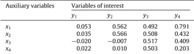
In each case, a sample is selected using the new method (Algorithm 1) and another one using Chauvet’s method with step 3 by landing phase by suppression of variables (Algorithm 2). For each sample, the total of the four variables of interest is estimated. The variance of the estimated total of the variables of interest is then computed conducting 10,000 simulations. In order to compare the results, the ratio of the variance of the estimated total of the variables of interest obtained using the new method (Algorithm 2) to the variance of the estimated total of the variables of interest obtained using Chauvet’s method with step 3 by landing phase by suppression of variables (Algorithm 1) is computed.Table 1presents the correlation between the variables of interest and the balancing variables. The results of the simulations are presented inTable 2.

In order to compare the execution time of both algorithms, a population of size 10,000, and the same balancing variables x1and x2as above are considered. The population is respectively partitioned into 25, 50, 100, 250, 500, and 1000 strata

of equal size. Samples of one unit per stratum balanced on the two balancing variables are selected with equal inclusion probabilities using Chauvet’s method with step 3 by landing phase by suppression of variables (Algorithm 1) and the new method (Algorithm 2). For each scenario, the mean time in seconds of selection of a sample and the failure rate of selection of a sample are observed for each method. One hundred samples are selected with each of the two methods to obtain these observations. The results are presented inTable 3.

Correlations between the variables of interest and the balancing variables.

Auxiliary variables Variables of interest

y1 y2 y3 y4 x1 0.053 0.562 0.492 0.791 x2 0.035 0.566 0.508 0.432 x3 −0.020 −0.007 0.517 0.409 x4 0.022 0.010 0.503 0.203 Table 2

Ratio of the variance of the estimated total of the variables of interest obtained using the new method (Algorithm 2) to the variance of the estimated total of the variables of interest obtained using Chauvet’s method with step 3 by landing phase by suppression of variables (Algorithm 1).

Variables of interest y1 y2 y3 y4 Case 1 0.974 0.985 0.991 1.019 Case 2 1.024 0.992 0.991 0.970 Case 3 1.016 0.980 1.047 1.065 Case 4 0.977 0.990 1.010 1.040 Table 3

Mean time in seconds and failure rate of selection of a sample with Chauvet’s method with step 3 by landing phase by suppression of variables (Algorithm 1) and with the new method (Algorithm 2) for 25, 50, 100, 250, 500, and 1000 strata and 1 unit selected in each stratum with equal inclusion probabilities.

Number of strata Algorithm 1 Algorithm 2

Mean time Failure rate Mean time Failure rate

25 1.883 0.00 1.941 0.00 50 2.066 0.00 2.108 0.00 100 2.805 0.00 2.289 0.00 250 22.451 0.00 2.959 0.00 500 387.126 0.03 4.039 0.00 1000 9770.745 0.13 6.656 0.00

Table 2shows that the new method (Algorithm 2) produces similar results in terms of variance of the estimated total as Chauvet’s method with step 3 by landing phase by suppression of variables (Algorithm 1). The new method has, however, the advantage over Chauvet’s method with step 3 by landing phase by suppression of variables. Indeed, an important gain in execution time arises if the new method is applied and selection of samples with highly stratified designs becomes tractable, as confirmed byTable 3. The original Chauvet’s method with step 3 by unequal probability sampling would, however, perform less well in terms of variance than the two methods with step 3 by landing phase by suppression of variables considered here. Indeed, a third step by unequal probability sampling would not take the balancing into account, which would result in a greater variance in the estimations.

8.2. Variance approximation formula and estimator

In order to study the performance of the proposed variance approximation formula and its estimator, the same balancing variables x1and x2and the same variables of interest y1to y4are considered. The population of size 1000 is partitioned into

25 equal size strata. Three scenarios are considered, namely the selection using the new method (Algorithm 2) of respectively 2 units, 4 units, and 8 units per stratum balanced on the two balancing variables. As above, the units are selected with equal inclusion probabilities. This results in samples of size 50, 100, and 200 respectively. For each scenario, the approximated variance is computed using formula(8). The simulation variance of the total estimatortyand the mean of the variance

estimator(9)are estimated drawing 10,000 samples for each scenario. The results are presented inTable 4.

The mean variance estimator almost matches the approximated variance. The estimator(9) is an almost unbiased estimator of the approximated variance(8). They are both close to the variance obtained by simulation. However, they tend to slightly underestimate the variance. The gap between the approximated variance and the simulated variance is due to the fact that the formula proposed byDeville and Tillé(2005) does not include the variance induced by the landing phase.

8.3. Illustration of the handling of nonresponse

An illustration of the use of the new method (Algorithm 2) in the context of nonresponse is shown here. Ilocos data set available in the R package ineq byZeileis(2013) is considered. The data shows household income in a region of the

Table 4

Approximated variance, mean of the variance estimator estimated using 10,000 simulations, and variance obtained by 10,000 simulations in the case of the estimation of the total of 4 variables of interest using the new method (Algorithm 2). Three cases are considered, namely the selection of samples of size n=50,100,200 respectively.

n Variables of interest

y1(×107) y2(×108) y3(×1011) y4(×1011)

50 Approximated var. 27.53 12.99 9.44 6.29

Mean var. estimator 27.23 12.95 9.58 6.39

Simulation var. 28.62 14.59 9.67 7.18

100 Approximated var. 13.04 6.15 4.48 2.99

Mean var. estimator 13.02 6.14 4.48 2.99

Simulation var. 13.15 6.54 4.58 3.24

200 Approximated var. 5.80 2.74 1.99 1.32

Mean var. estimator 5.79 2.74 1.99 1.33

Simulation var. 5.66 2.90 2.01 1.40

Philippines called Ilocos and comes from two Philippines’ National Statistics Office surveys. The data coming from the 1998 Annual Poverty Indicators Survey are considered here. The sample size is 632. Five domains Dhfor h

=

1

, . . . ,

5 are created

by grouping households by family size (variable AP.family.size). Each domain, except the last one, refers to 2 consecutive family sizes. The first domain D1therefore contains the households whose family size lies in

{1

,

2}, the second domain D2

contains the households whose family size lies in

{3

,

4}, and so on until the fourth domain. The fifth domain contains the households whose family size exceeds 8. The variable of interest y is the income (variable AP.income) and xkis the vector

of domain indicators. A respondents set is created by generating a response indicator vector r

=

(

rk

),

k

∈

S. For k

∈

S, the

component rkis generated from a Bernoulli random variable with parameters 0.55, 0.60, 0.65, 0.70, or 0.75 if the unit k

∈

S

belongs to domain D1

,

D2

,

D3

,

D4, or D5respectively (uniform nonresponse mechanism inside the domains). This results in

an overall mean response rate of 0.60.

Then 1000 hot-deck and survey weighted imputations are conducted by the method proposed inChauvet et al.(2011b) and presented in Section7.3. The new method (Algorithm 2) is applied as explained in Section7.4to obtain the imputed values. For each imputation, the imputed estimator



θ

I

=









k∈Dh dkrkyk

+



k∈Dh dk

(

1

−

rk

)

y∗k



k∈Dh dk







1≤h≤5

,

for the vector of domain means

θ = 

Y1

, . . . ,

Y5



is computed. Let



θ

_Iibe the imputed estimate of simulation i. To check that the imputation variance of



θ

_Iis eliminated (or almost), the vector of relative root imputation variances (RRIV) defined as

RRIV





θ

I

 =











1 999 1000



i=1





θ

_Ii

−

1 1000 1000



i=1



θ

_Ii



2



θ

,

where



θ =









k∈Dh d_ky_k



k∈Dh dk







1≤h≤5

,

is computed.Table 5presents the results. It shows that the RRIV is almost eliminated through balanced random imputation with the new method (Algorithm 2).

9. Conclusion

In this paper, a new algorithm for stratified balanced sampling has been proposed. This algorithm selects samples which are approximately balanced in each stratum, balanced across the entire population and such that a fixed number of units is selected in each stratum. It is faster and more resistant to numerical instability than the previous methods proposed in this context. Moreover, this new algorithm greatly reduces the number of variables considered in the balancing procedures. Therefore, it makes it possible to select stratified balanced samples in some highly stratified populations that could not be handled using existing methods. A variance approximation formula for the total and its estimator have been proposed. A possible application of the new method to the handling of nonresponse has been provided. Finally, results of a simulation study have confirmed the performance of the proposed method, the accuracy of the formula for the variance approximation and its estimator, and the usefulness of the method for the handling of nonresponse.

Table 5

Relative root imputation variance (RRIV) of the imputed estimator for a vector of domain means obtained through balanced random imputation using the new method (Algorithm 2).

Domain RRIV 1 4.60·10−07 2 7.58·10−08 3 4.66·10−08 4 1.21·10−07 5 2.22·10−07 Acknowledgments

The authors wish to thank the associate editor and the three reviewers for their useful and constructive comments and suggestions, which helped to considerably improve this manuscript. This research was supported by the Swiss federal statistical office.

Appendix. Proof of the result (i) Proof by induction.

(a) For j

=

2 in step 2 of Algorithm 2, two strata are considered. Therefore q

+

2 balancing variables are used in the flight phase. Thus

#



k

∈

U1

∪

U2

|0

< φ

(k2)

<

1



≤

q

+

2

≤

2q

+

2

.

The result is valid for j

=

2.

(b) Assume that the result is valid for j

=

ℓ

, i.e. assume that #



k

∈

ℓ



i=1 Ui











0

< φ

(ℓ)_k

<

1



≤

2q

+

2

.

As it is impossible to have a rounding problem for a single unit of a stratum (the sum of the inclusion probabilities is an integer in each stratum), the number of strata containing units such that 0

< φ

(ℓ)_k

<

1 is at most q

+

1. Then a strata is added for the flight phase for step j

=

ℓ +

1. Therefore, at most q

+

2 strata are considered, which means that at most q

+

2 balancing variables of the type of

φ

_k(j−1)

1

(

k

∈

Ui

)

are required. Moreover, the q

balancing variables

φ

(j−1) k x ⊤ k

π

k

are considered. In total, at most 2q

+

2 balancing variables are used in the flight phase for j

=

ℓ +

1. This implies that #



k

∈

ℓ+1



i=1 Ui











0

< φ

(ℓ+_k 1)

<

1



≤

2q

+

2

,

which means that the result is true for j

=

ℓ +

1.

(ii) Z(j)represents the matrix whose columns are the balancing variables used in the jth flight phase of step 2 of Algorithm 2. In the previous point, it is shown that at most 2q

+

2 units are considered in each flight phase of step 2. It has also been explained that, in total, at most 2q

+

2 balancing variables are used in each of these flight phases. It results that the number of non-null columns of matrix Z(j)is less than or equal to 2q

+

2.

References

Baillargeon, S., Rivest, L.P., 2011. Stratification: univariate stratification of survey populationcs. URL: http://CRAN.R-project.org/package=stratification, R Package Version 2.0-3.

Brewer, K.R.W., 1999. Design-based or prediction-based inference? Stratified random vs stratified balanced sampling. Internat. Statist. Rev. 67, 35–47. Bülher, W., Deutler, T., 1975. Optimal stratification and grouping by dynamic programming. Metrika 22, 161–175.

Chauvet, G., 2009. Stratified balanced sampling. Surv. Methodol. 35, 115–119.

Chauvet, G., Bonnéry, D., Deville, J.C., 2011a. Optimal inclusion probabilities for balanced sampling. J. Statist. Plann. Inference 141, 984–994. Chauvet, G., Deville, J.C., Haziza, D., 2011b. On balanced random imputation in surveys. Biometrika 98, 459–471.

Chauvet, G., Tillé, Y., 2006. A fast algorithm of balanced sampling. J. Comput. Statist. 21, 9–31. Dalenius, T., Hodges, J.L.J., 1959. Minimum variance stratification. J. Amer. Statist. Assoc. 54, 88–101.

Deville, J.C., Grosbras, J.M., Roth, N., 1988. Efficient sampling algorithms and balanced sample. In: COMPSTAT, Proceedings in Computational Statistics. Physica Verlag, Heidelberg, pp. 255–266.

Deville, J.C., Tillé, Y., 2004. Efficient balanced sampling: the cube method. Biometrika 91, 893–912.

Deville, J.C., Tillé, Y., 2005. Variance approximation under balanced sampling. J. Statist. Plann. Inference 128, 569–591.

Díaz-García, J.A., Garay-Tápia, M.M., 2007. Optimum allocation in stratified surveys: stochastic programming. Comput. Statist. Data Anal. 51, 3016–3026. Grafström, A., Matei, A., Qualité, L., Tillé, Y., 2012. Size constrained unequal probability sampling with a non-integer sum of inclusion probabilities. Electron.

Horvitz, D.G., Thompson, D.J., 1952. A generalization of sampling without replacement from a finite universe. J. Amer. Statist. Assoc. 47, 663–685. Kalton, G., Kish, L., 1984. Some efficient random imputation methods. Commun. Stat. A13, 1919–1939.

Lavallée, P., Hidiroglou, M.A., 1988. On the stratification of skewed populations, sur la stratification de populations asymétriques. Surv. Methodol. Tech. d’enquête 14, 35–45.

Nedyalkova, D., Tillé, Y., 2008. Optimal sampling and estimation strategies under linear model. Biometrika 95, 521–537.

Neyman, J., 1934. On the two different aspects of the representative method: the method of stratified sampling and the method of purposive selection. J. Roy. Statist. Soc. 97, 558–606.

Tillé, Y., Favre, A.C., 2005. Optimal allocation in balanced sampling. Statist. Probab. Lett. 74, 31–37. Wolter, K.M., 1985. Introduction to Variance Estimation. Springer, New York.

Wright, T., 2012. The equivalence of neyman optimum allocation for sampling and equal proportions for apportioning the US house of representatives. Amer. Statist. 66 (4), 217–224.