Coordinated ground-based and Cluster observations of large amplitude global magnetospheric oscillations during a fast solar wind speed interval

HAL Id: hal-00316958

https://hal.archives-ouvertes.fr/hal-00316958

Submitted on 1 Jan 2002

HAL is a multi-disciplinary open access

archive for the deposit and dissemination of

sci-entific research documents, whether they are

pub-lished or not. The documents may come from

teaching and research institutions in France or

abroad, or from public or private research centers.

L’archive ouverte pluridisciplinaire HAL, est

destinée au dépôt et à la diffusion de documents

scientifiques de niveau recherche, publiés ou non,

émanant des établissements d’enseignement et de

recherche français ou étrangers, des laboratoires

publics ou privés.

large amplitude global magnetospheric oscillations

during a fast solar wind speed interval

I. R. Mann, I. Voronkov, M. Dunlop, E. Donovan, T. K. Yeoman, D. K.

Milling, J. Wild, K. Kauristie, O. Amm, S. D. Bale, et al.

To cite this version:

I. R. Mann, I. Voronkov, M. Dunlop, E. Donovan, T. K. Yeoman, et al.. Coordinated ground-based

and Cluster observations of large amplitude global magnetospheric oscillations during a fast solar

wind speed interval. Annales Geophysicae, European Geosciences Union, 2002, 20 (4), pp.405-426.

�hal-00316958�

Annales

Geophysicae

Coordinated ground-based and Cluster observations of large

amplitude global magnetospheric oscillations during a fast solar

wind speed interval

I. R. Mann1, I. Voronkov2, M. Dunlop3, E. Donovan4, T. K. Yeoman5, D. K. Milling1, J. Wild5, K. Kauristie6, O. Amm6, S. D. Bale7, A. Balogh3, A. Viljanen6, and H. J. Opgenoorth8

1_{Department of Physics, University of York, York, UK}

2_{Department of Physics, University of Alberta, Edmonton, Alberta, Canada} 3_{Imperial College, London, UK}

4_{Department of Physics and Astronomy, University of Calgary, Alberta, Canada} 5_{Department of Physics and Astronomy, University of Leicester, Leicester, UK}

6_{Finnish Meteorological Institute, Geophysical Research Division, P.O. Box 503, FIN-00101, Helsinki, Finland} 7_{Space Sciences Laboratory, University of California, Berkeley, USA}

8_{Swedish Institute of Space Physics, Uppsala Division, Sweden}

Received: 18 June 2001 – Revised: 24 September 2001 – Accepted: 16 October 2001

Abstract. We present magnetospheric observations of very

large amplitude global scale ULF waves, from 9 and 10 De-cember 2000 when the upstream solar wind speed exceeded 600 km/s. We characterise these ULF waves using ground-based magnetometer, radar and optical instrumentation on both the dawn and dusk flanks; we find evidence to sup-port the hypothesis that discrete frequency field line reso-nances (FLRs) were being driven by magnetospheric waveg-uide modes. During the early part of this interval, Clus-ter was on an outbound pass from the northern dusk side magnetospheric lobe into the magnetosheath, local-time con-jugate to the Canadian sector. In situ magnetic fluctua-tions, observed by Cluster FGM, show evidence of quasi-periodic motion of the magnetosheath boundary layer with the same period as the ULF waves seen on the ground. Our observations represent the first simultaneous magnetome-ter, radar and optical observations of the characteristics of FLRs, and confirm the potential importance of ULF waves for magnetosphere-ionosphere coupling, particularly via the generation and modulation of electron precipitation into the ionosphere. The in situ Cluster measurements support the hypothesis that, during intervals of fast solar wind speed, the Kelvin-Helmholtz instability (KHI) can excite spheric waveguide modes which bathe the flank magneto-sphere with discrete frequency ULF wave power and drive large amplitude FLRs.

Paper submitted to the special issue devoted to “Cluster: First scientific results”, Ann. Geophysicae, 19, 10/11/12, 2001.

Key words. Magnetospheric physics (magnetopause, cusp

Correspondence to: I. R. Mann (ian@aurora.york.ac.uk)

and boundary layers; MHD waves and instabilities; solar wind-magnetosphere interactions)

1 Introduction

Global oscillations of magnetospheric field lines can be ex-cited in the magnetosphere by the solar wind. Dungey (1955) was the first to consider the possibility that ultra-low fre-quency (ULF) waves might constitute Alfv´en waves which stand along geomagnetic field lines. Southwood (1974) and Chen and Hasegawa (1974) first considered how fast surface waves, excited by the Kelvin-Helmholtz instability (KHI) on the magnetopause, could drive standing Alfv´en field line resonances (FLRs) on field lines of matching eigen-frequency. Following the observations of Kivelson et al. (1984), Kivelson and Southwood (1985, 1986) solved the problem of explaining the occurrence of discrete frequency FLRs by proposing that radially standing fast cavity mode waves could be excited between the magnetopause and a turning point inside the magnetosphere. Their model pro-duced a discrete spectrum of cavity modes, each of which would resonantly drive a monochromatic FLR. Later work (see e.g. Samson et al., 1992; Walker et al., 1992; Wright, 1994) proposed that the outer magnetosphere might be bet-ter modelled as an open waveguide, rather than a cavity. In the waveguide model, discrete frequency wavegui de modes drive FLRs as they propagate and disperse down the waveg-uide, Mann et al. (1998) having presented the first

observa-tional evidence for the existence and propagation of waveg-uide modes.

In recent theoretical work, Mann et al. (1999) showed how, under conditions of sufficiently fast magnetosheath flow speed, body type magnetospheric waveguide modes can be driven by magnetopause KHI, in addition to the standard KH surface waves (see also Mills et al., 1999). Interestingly, the Mann et al. (1999) theory predicts that the conditions lo-cal to the magnetopause can control both the transport ULF wave power from the magnetosheath into the magnetosphere and the excitation of large amplitude FLRs. By examining the azimuthal phase speed characteristics of multiple har-monic FLRs, the Mann et al. (1999) theory can also be used to distinguish between FLRs driven by waveguide modes which result from solar wind impulses and those waveguide modes which are excited by magnetopause KHI (see Mann and Wright, 1999; Mills and Wright, and Mathie and Mann, 2000, for more details).

To test this theory requires ground-satellite conjugate stud-ies which compare the global structure of the FLRs seen on the ground with satellite measurements from close to the magnetopause. In this paper we conduct co-ordinated ground-based and Cluster observations of the global scale Pc5 ULF waves which are excited on the magnetospheric flanks between 9 and 10 December 2000 during an inter-val of fast (> 600 kms−1) solar wind speed. Our observa-tions provide support for the hypotheiss that the KHI was responsible for exciting the large amplitude pulsations ob-served on the ground and for injecting significant energy into the flank magnetosphere. Our observations also provide fur-ther supporting evidence for the importance of ULF waves for magnetosphere-ionosphere coupling, in particular though the generation of auroral currents and the modulation of elec-tron precipitation into the auroral ionosphere.

2 Instrumentation

We present co-ordinated ground-based and Cluster observa-tions of ULF pulsaobserva-tions from 22:00 UT on 9 December (day of year 344) until 08:00 UT on 10 December 2000 (day of year 345). During this interval the magnetosphere was sub-ject to a steady fast solar wind speed stream, the level 2 ACE data from the SWEPAM (McComas et al., 1998) instrument (not shown) showing that the solar wind speed remained in excess of 600 km/s, the solar wind dynamic pressure remain-ing constant ∼ 2.5 nPa. Between approximately 22:00 UT and 02:00 UT, the Saskatoon SuperDARN radar (Greenwald et al., 1995), and CANOPUS (Rostoker et al., 1995) magne-tometer and phomagne-tometer data from the dusk local time sector showed clear evidence of the excitation Pc5 FLRs.

During December 2000, the Cluster spacecraft were still in the commissioning phase; however, data was being taken during certain intervals. Between approximately 22:00 UT and 24:00 UT, Cluster was local-time conjugate to the Cana-dian sector on an outbound trajectory from the northern dusk flank lobe into the magnetosheath. Figure 1 shows the

po-sitions of the CANOPUS stations (red dots in the Canadian sector) and the field of view of the Saskatoon SuperDARN radar in the Canadian sector. Filled dots indicate the mag-netic footprint of the Cluster 1 satellite trajectory, traced with the Tsyganenko 96 field model (Tsyganenko, 1996), plotted every 5 min and colour coded to indicate the radial position of the spacecraft. Similarly, un-filled dots show the radial projection of the trajectory of Cluster 1 and demonstrate the local time conjugacy of the Cluster satellites to the Canadian sector. The geographic pole is indicated with a cross; con-tours of geomagnetic latitude and longitude are plotted with increments of 10 and 15 degrees, respectively.

Later in this interval, from 01:30 UT until around 08:00 UT (and later), the morning local time sector showed clear evidence from European ground instrumentation of large amplitude pulsations and field line resonances. The field of view of the STARE Norway radar (belonging to the MIRACLE instrument network, Syrj¨asuo et al., 1998), and the CUTLASS (Co-operative UK Twin Located Auroral Sounding System) Hankasalmi, Finland (26.61◦_{E, 62.32}◦_N)

SuperDARN radar, along with the positions of the IMAGE (L¨uhr et al., 1998) and SAMNET (Yeoman et al., 1990a) magnetometer stations (red dots in the European sector) used in this study are also indicated on Fig. 1. The geographic and magnetic coordinates of the CANOPUS and the IMAGE and SAMNET magnetometer stations are given in Tables 1 and 2 respectively. This configuration of ground-based instruments on the dawn and dusk flank, combined with data local to the dusk magnetopause from Cluster, allow us to present a de-tailed analysis of the energisation of both the dawn and dusk flank magnetosphere (e.g. McDiarmid et al., 1994) by the solar wind. The Cluster data allow us to test the hypothesis that fluctuations close to the magnetopause, such as the KHI, may have energised large amplitude pulsations and field line resonances on the flanks of the magnetosphere.

3 Observations

3.1 Ground-based dusk sector observations

We use Canadian sector ground-based data to identify and characterize a well-defined field line resonance and the as-sociated wave dynamics in the dusk sector. Pc5 wave activ-ity is evident in CANOPUS magnetometer data in the hours between 22:00 UT on 9 December and 04:00 UT on 10 De-cember 2000. As we have supporting SuperDARN radar and CANOPUS photometer data, we focus on the latter part of this interval. Figure 2 shows the H and D components of the magnetic field measured by the CANOPUS magnetometer network from 00:00–04:00 UT, the data having been rotated from geographic X and Y polarisation into CGM H and D magnetic polarisation for the year 2000 epoch. Large am-plitude Pc5 ULF wave activity is clearly visible throughout this interval in both the H and D components, with a particu-larly prominent wave packet being observed between 00:00– 00:40 UT. Figure 2 also clearly shows that the ULF wave

ac-Table 1. The coordinates of the CANOPUS magnetometer stations used in this study. The corrected geomagnetic coordinates (CGM) were calculated for the 2000 epoch at an altitude of 120 km using the International Geomagnetic Reference Field converter at http://nssdc.gsfc.gov/space/cgm/cgm.html

Stations Geodetic CGM

Station Code Latitude Longitude Latitude Longitude

Taloyoak TAL 69.54 266.45 78.97 328.97

Contwoyto Lake CON 65.75 248.75 73.25 302.67

Rankin Inlet RAN 62.82 267.89 72.91 334.76

Eskimo Point ESK 61.11 265.95 71.20 331.90

Fort Churchill FCH 58.76 265.92 68.99 332.38

Fort Smith FSM 60.02 248.05 67.71 305.28

Rabbit Lake RAB 58.22 256.32 67.38 317.70

Fort Simpson FSI 61.76 238.77 67.53 292.55

Gillam GIL 56.38 265.36 66.69 331.95

Dawson DAW 64.05 220.89 66.00 272.23

Fort McMurray MCM 56.66 248.79 64.60 307.80

Island Lake ISL 53.86 265.34 64.26 332.32

Pinawa PIN 50.20 263.96 60.56 330.76

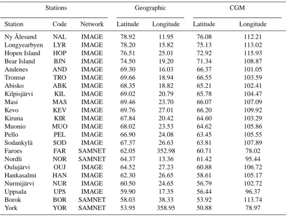
Table 2. The coordinates of the IMAGE and SAMNET magnetometer stations used in this study. The corrected geomagnetic coordinates

(CGM) were calculated for the 2000 epoch at an altitude of 120 km using the International Geomagnetic Reference Field converter at http://nssdc.gsfc.gov/space/cgm/cgm.html

Stations Geographic CGM

Station Code Network Latitude Longitude Latitude Longitude

Ny ˚Alesund NAL IMAGE 78.92 11.95 76.08 112.21

Longyearbyen LYR IMAGE 78.20 15.82 75.13 113.02

Hopen Island HOP IMAGE 76.51 25.01 72.92 115.93

Bear Island BJN IMAGE 74.50 19.20 71.34 108.87

Andenes AND IMAGE 69.30 16.03 66.37 101.05

Tromsø TRO IMAGE 69.66 18.94 66.55 103.59

Abisko ABK IMAGE 68.35 18.82 65.21 102.41

Kilpisj¨arvi KIL IMAGE 69.02 20.79 65.78 104.47

Masi MAS IMAGE 69.46 23.70 66.07 107.09

Kevo KEV IMAGE 69.76 27.01 66.20 109.92

Kiruna KIR IMAGE 67.84 20.42 64.60 103.29

Muonio MUO IMAGE 68.02 23.53 64.62 105.86

Pello PEL IMAGE 66.90 24.08 63.45 105.55

Sodankyl¨a SOD IMAGE 67.37 26.63 63.81 107.89

Faroes FAR SAMNET 62.05 352.98 60.71 78.02

Nordli NOR SAMNET 64.37 13.36 61.42 95.44

Ouluj¨arvi OUJ IMAGE 64.52 27.23 60.88 106.72

Hankasalmi HAN IMAGE 62.30 26.65 58.61 105.17

Nurmij¨arvi NUR IMAGE 60.50 24.65 56.79 102.72

Uppsala UPS IMAGE 59.90 17.35 56.44 96.37

Borok BOR SAMNET 58.03 38.33 53.92 113.74

York YOR SAMNET 53.95 358.95 50.88 78.97

tivity is stronger over the eastern CANOPUS stations, the waves being much less apparent at the most (CGM) longitu-dinally distant stations DAW, FSM and FSI.

Figure 3 shows the (CGM) latitudinally stacked H compo-nent power spectrum for the interval 00:00–01:00 UT, filtered

between 1 and 10 mHz (note that the DAW power spectra is not shown due to the low wave amplitudes and this sta-tion’s large longitudinal separation from the other CANO-PUS sites). Between the latitudes of the FCH and MCM stations, a very clear latitude independent spectral peak at

MODEL PARAMETERS: T96 field model IMF By: 0.0 nT IMF Bz: -2.0 nT PSW: 2.2 nPa Dst: 0 Footprint alt: 100.0 km 18 UT 19 UT 20 UT 21 UT 00 UT 01 UT 18 UT 19 UT 20 UT 21 UT 22 UT 23 UT 00 UT 01 UT 02 UT 22 UT 23 UT 2 4 6 8 10 12 14 16 18

Radial position (R

₎

Fig. 1. Ground track of Cluster 1. Filled

dots indicate the magnetic footprint, traced with the Tsyganenko (1996) field model, whilst unfilled dots indicate the radial projection of the Cluster 1 tra-jectory, colour coded with the satellites

radial position. Also shown are the

locations of the CANOPUS, IMAGE and SAMNET magnetometers, along with the fields of view of the CUT-LASS Finland and Saskatoon Super-DARN radars, as well as that of the STARE Norway radar.

around 3.0 mHz is apparent, the half power points spanning approximately 2.8–3.4 mHz. In Fig. 4, we show the results from a complex demodulation analysis (e.g. Beamish et al., 1979) of this dominant spectral peak. The technique of com-plex demodulation allows one to determine the amplitude and phase characteristics of a non-stationary time series by comparison with a reference signal. Figure 4 shows the latitudinal variation of the H and D component amplitude (first panel) and phase (second panel) for the CANOPUS Churchill line at the time of maximum H component am-plitude (6 min period demodulate, bandpass filtered between 341 s and 381 s and analysed at 00:20 UT; see Mathie et al. (1999) for more details about applying the complex demod-ulation technique to FLRs).

For the dominantly Alfv´enic signatures expected at a field line resonance, the magnetic perturbations in the magneto-sphere are rotated through 90◦ upon transmission through the ionosphere to the ground (e.g. Hughes and Southwood, 1976). Consequently, a well-developed FLR with a dominant toroidal polarisation in the magnetosphere would be rotated into a wave dominated by the H -component on the ground, exactly as is seen in Fig. 4. The H -component shows the clear latitudinal amplitude maxima and 180◦_{phase change}

expected for a well-developed field line resonance (see e.g. Mathie et al., 1999). The D-component also shows an ampli-tude maximum, and similarly displays a large phase change across the resonance.

The dominant wavepacket is bestdefined in the H -component for the stations FSM, GIL and RAB. Using the maximum H -component demodulate from RAB and GIL gives a dimensionless azimuthal wavenumber m ∼

0.5 ± 0.3 (the error, calculated from the CANOPUS sam-pling rate, probably gives an upper bound; using an aver-age over the three maximum amplitude demodulates gives

m ∼ 0.4 ± 0.1, the error being the standard deviation). Us-ing the D-component, away from the resonance, can min-imise any phase changes arising due to small latitudinal dis-placements between longitudinally spaced stations. Using the D-component station pair of ISL and MCM, away from the resonance, gives m = +1.7 ± 0.2 (the H -component gives m = +1.5 ± 0.2). Despite the slight variability, all these measurements are consistent with the expected east-ward (taileast-ward) propagation for dusk FLRs which are excited by waveguide modes driven by the solar wind. The low mag-nitude of m is consistent with previous observations of FLRs which were believed to have been driven by magnetospheric waveguide modes (e.g. Fenrich et al., 1995; Mathie et al., 1999) and signifies that the waves are global scale magneto-spheric phenomena.

In Fig. 5 we show in more detail the latitudinal dynam-ics of the pulsations along the Churchill line. The top panel shows a keogram of 557.7 nm data from the CANOPUS Rankin Inlet meridian scanning photometer (MSP) while the bottom panel shows a stack plot of the X-component magne-tometer data from the six Churchill line magnemagne-tometer sta-tions (AACGM, e.g. Baker and Wing, 1989, invariant lati-tudes from 65◦to 80◦), plotted on the same amplitude scale and band-pass filtered between 60 and 660 s. Both the mag-netometer and MSP data show that Pc5 wave activity exists on magnetic latitudes up to Rankin Inlet. More interestingly, the phase of the X-component magnetic fields shows the clear polewards phase propagation which is expected for a

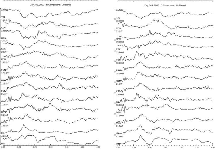
0.00 0.40 1.20 2.00 2.40 3.20 4.00

Day 345, 2000 : H Component : Unfiltered 104.0nT TAL 102.0nT CON 194.0nT RAN 370nT ESK 280nT FCH 156.0nT FSM 178.0nT RAB 112.0nT FSI 256nT GIL 116.0nT DAW 98.5nT MCM 138.0nT ISL 45.0nT PIN 0.00 0.40 1.20 2.00 2.40 3.20 4.00

Day 345, 2000 : D Component : Unfiltered 98.0nT TAL 150.0nT CON 232nT RAN 198.0nT ESK 126.0nT FCH 184.0nT FSM 152.0nT RAB 216nT FSI 130.0nT GIL 184.0nT DAW 112.0nT MCM 91.5nT ISL 57.0nT PIN

Fig. 2. Stacked raw H (a) and D (b) magnetograms from the CANOPUS magnetometer network between 00:00 UT and 04:00 UT on 10

December 2000.

driven field line resonance (e.g. Wright and Allan, 1996a). The 630 nm data from the Rankin Inlet MSP (not shown) indicates that the boundary between open and closed field-lines lies at ∼ 74◦AACGM invariant between 00:00 UT and 01:00 UT, after which it moves poleward (see Blanchard et al., 1997, for a discussion of the use of 630 nm data in the determination of the polar cap boundary). Hence, during the interval 00:00–01:00 UT, the peak 557.7 nm emissions are located roughly 2◦ equatorward of the polar cap boundary (between the latitudes of the ESK and RAN magnetometer stations). This is consistent with Figs. 2, 3 and 5 which show that the highest latitude station TAL displays very little evi-dence of any clear ULF wave activity, consistent with its lo-cation on open field lines inside the polar cap. Moreover, the 630 nm data suggest that the latitude of the resonance maps into the central plasma sheet.

In Fig. 6 we show the ionospheric F-region plasma veloc-ity as measured by beam 14 of the Saskatoon SuperDARN radar. Positive velocities correspond to motion towards the radar. As beam 14 of the radar passes over Fort Churchill (see Fig. 1 of Voronkov et al. (1997) for a schematic of relative positions of the SuperDARN field of view over the Churchill Line stations), positive velocities are indicative of south-west

oriented plasma drifts. As can be seen in Fig. 6, there is a clear signature of a field line resonance in the radar data be-tween 00:00 UT and 00:30 UT. Furthermore, comparing ve-locities measured in different beams, we can conclude that the resonance is dominantly polarised with the flow velocity in the azimuthal direction. Based on the SuperDARN data, the phase of the pulsations clearly increases with increasing latitude, again consistent with the poleward phase propaga-tion seen in the X-component magnetometer data in Fig. 5.

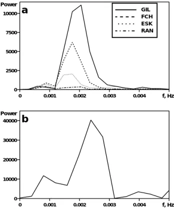
Magnetometer and radar data are further analysed in Fig. 7 where the power spectral density of the X-component mag-netic field from GIL, FCH, ESK, and RAN is shown in panel (a), and the power spectral density of plasma velocity from beam 14 of the Saskatoon radar is shown in panel (b). The data have been pre-filtered with a Butter filter with a low frequency cutoff at 0.5 mHz. The magnetometer data shows that the frequency of the spectral peak at each station de-creases with latitude, again, as expected for a driven field line resonance. For a driven resonance, the response on any given field line will result from a combination of the fast mode driv-ing frequency and the local natural Alfv´en frequency of the field line (see e.g. ?, and references therein for a detailed dis-cussion)McDiarmid++99. Once the driver has decayed, the

0 1 2 3 4 5 6 7 8 Frequency (mHz)

POWER (Arbitrary Units, independently scaled)

TAL

0 200

Day 345, 0 0: 0 for 60 minutes

H Component : Filtered 1000 to 100 s : Smoothed over 1 Estimates

CON 0 200 RAN 0 200 ESK 0 200 FCH 0 200 400 FSM 0 500 RAB 0 500 FSI 0 200 400 GIL 0 200 400 MCM 0 500 ISL 0 200 400 PIN 0 500

Fig. 3. CANOPUS stacked H -component power spectra (filtered from 1–10 mHz) from 00:00 UT to 01:00 UT on 10 December 2000.

field line resonance will be increasingly dominated by the re-sponse at the local Alfv´en resonant eigenfrequency. This will result in phase mixing across the FLR (see e.g. Mann et al., 1995). The increase of wave period with latitude, character-istic of phase mixing, is the most expected and important fea-ture of a well-developed field line resonance and is a direct consequence of an Earthward gradient of the Alfv´en velocity in the magnetosphere outside the plasmapause. In panel (b), it can be clearly seen that the spectral distribution of the con-vection pulsations measured by the radar is close to the spec-trum of magnetic pulsations registered by the Fort Churchill magnetometer, confirming that both instruments are measur-ing the same wave at the same location.

Observations of the field line resonance above are in very good agreement with theoretical expectations such as those presented Samson et al. (1998) which can be summarized as follows. At one phase of the resonance, the upward field

aligned current (FAC) sheet is at the equatorward border of the resonance region. This FAC moves poleward, consis-tent with the latitudinal phase shift (c.f. Wright and Allan, 1996a and Mann, 1997). In the low-m field line resonance, the upward FAC is mostly closed by a near-longitudinally directed Pedersen current. This in turn corresponds to an Eastward Hall current equatorward of the upward FAC sheet. The maxima of the Eastward Hall current occurs at the same time as the peak of the westward plasma convection flow. In Fig. 8, we combine the time dependence of the mag-netic X-component Fort Churchill (normalized by 100 nT) and plasma velocities measured using beam 14 right above Fort Churchill. As seen from Fig. 8, these independent instruments show excellent agreement with both the mag-netic and velocity measurements showing the same period and wavepacket structure. Moreover, the observed velocities and X-component magnetic field perturbations are clearly in

Fig. 4. Complex demodulation latitudinal amplitude (first panel)

and phase (second panel) variations of the H and D-components of the 2.8 mHz wave along the CANOPUS Churchill line, centred on 00:20 UT. 0000 0020 0040 0100 0120 0140 0200 UT (hours) TAL RAN ESK FCH GIL ISL

Fig. 5. CANOPUS pulsation activity between 00:00 UT and 02:00 UT on 10 December 2000: 557.7-nm emission intensity ob-served by the Rankin Inlet MSP as a function of AACGM invariant latitude (top panel) and stacked X-component magnetogram time series (bandpassed between 60–660 s) from the Churchill line mag-netometers (bottom panel).

phase, as expected on the basis of the above arguments. 3.2 Cluster dusk sector observations

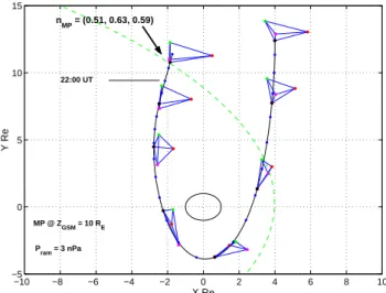
At 22:00 UT on 9 December, Cluster was on an outbound trajectory through the northern lobe in the dusk flank, conju-gate to the Canadian sector on the ground (see Fig. 1). Fig-ure 9 shows the trajectory of the four Cluster spacecraft in the GSE X − Y plane, with blue dots marking the positon of Cluster 1 every hour. The spacecraft separations are in-creased by a factor of 20 to show their geometrical config-uration and the position of Cluster at 22:00 UT is indicated. Between 22:00–24:00 UT Cluster remained close to constant

Z at around Z = 9 RE. The location of a model

magne-Date: 01210, SDARN Doppler Radar, Stn = Saskatoon, b14

0:00 0:30 1:00 1:30 2:00 Time UT 66 68 70 72 74 76 aacgm Latitude -500. 500. vel m/s both

Fig. 6. Velocity in the ionospheric F -region along beam 14 of the

SuperDARN Saskatoon radar between 00:00 UT and 02:00 UT on 10 December 2000. Positive velocities are in the direction toward the radar (close to the south-west direction above Fort Churchill).

0 0.001 0.002 0.003 0.004 0.005 0 2500 5000 7500 10000

a

b

Fig. 7. Power spectral densities of the X-component magnetic field

from selected magnetometer stations along the Churchill line (a), and from beam 14 of the Saksatoon SuperDARN radar at the range

gate at 70◦above the Fort Churchill (FCH) magnetometer station

(b). Spectra were taken for the interval 00:00 UT and 00:40 UT with

an FFT, pre-filtered with a Butter filter with a cutoff at 0.5 mHz.

topause, for an upstream dynamic pressure of 3 nPa, is also shown in the GSE X−Y plane at a fixed height of Z = 10 RE

(GSM). The vector direction of the magnetopause, normal (GSE) from the model at the location crossed by Cluster, is also indicated (nMP =(0.51, 0.63, 0.59)).

In Fig. 10 we show the magnetic field measured by the FGM instrument (Balogh et al., 2001) on-board Cluster 3 be-tween 21:00 and 24:00 UT on 9 December 2000. The first, second and third panels show the spin resolution 4 s FGM magnetic field in the GSE Z, Y and X directions,

respec-UT, min 0 10 20 30 40 -1 0 1 V/(1000 m/s) X/(100 nt) X/(100 nT)

Fig. 8. Velocity (normalised by 1000 m/s) in the ionospheric F

-region recorded by the Saskatoon radar (beam 14) at the latitude of Fort Churchill and magnetic X-component data (normalised by 100 nT) from Fort Churchill.

tively, with the final panel showing the magnetic field mag-nitude. As can be clearly seen, Cluster enters the magne-tosheath boundary layer from the magnetosphere at 22:10 UT (first dotted red line, marked as BL). At 23:40 UT, Clus-ter crosses the magnetopause and enClus-ters the magnetosheath proper (second dotted red line, marked as MP). Between these times, Cluster travels deeper into the magnetosheath boundary layer, the magnetic field gradually decreasing from magnetospheric values (before 22:10 UT) towards the lower magnetosheath magnetic fields seen at the end of the interval (after 23:40 UT).

In Fig. 11 we show the results from a minimum vari-ance analysis (Sonnerup and Cahill, 1967) of the magne-topause crossing around 23:40 UT which shows significant shear across the boundary. The top panel shows, after Dun-lop et al. (1999), a scatter plot (pink crosses) of the mag-netic field angles (θ and φ GSE) measured by FGM on Clus-ter 2 between 23:34–23:48 UT. For a tangential discontinu-ity (TD) crossing, the field direction through the boundary should lie nearly on a plane (since B.n = 0). The green curve represents a planar fit to the data points, indicating the field directions which would be expected if the mag-netic field vectors during this magnetopause crossing lay in a plane. The red curve shows the locus of the plane which results from a minimum variance analysis (MVA) between these times, the minimum variance plane having a normal vector nMV A = (0.63, 0.49, 0.60) (GSE). The normal

di-rection is stable and has an eigenvalue ratio in excess of 10. There is excellent agreement between the fit to the observed data and the results from the minimum variance analysis in-dicating that the magnetopause was a fairly clean tangential discontinuity.

Interestingly, MVA analysis applied to Cluster 1 and Clus-ter 3 in the same inClus-terval produces normals which point in the same direction as Cluster 2 (Cluster 1 nMV A =

[0.64, 0.50, 0.59]; Cluster 3 nMV A = [0.64, 0.51, 0.58]).

Cluster 4 produces a slightly different normal, tilting slightly

−10 −8 −6 −4 −2 0 2 4 6 8 10 −5 0 5 10 15 Y Re X Re 22:00 UT MP @ ZGSM = 10 RE Pram = 3 nPa n MP = (0.51, 0.63, 0.59)

Fig. 9. Cluster trajectory in the GSE X − Y plane, at a constant Z

GSM of 10 REon 9 December 2000 (black, red, green and magneta

represent the Cluster 1, 2, 3 and 4 spacecraft respectively, and the spacecraft separations are magnified by a factor of 20). The posi-tion of a model magnetopause for a 3 nPa dynamic pressure, and the location of Cluster 1 at 22:00 UT is also shown. Also indicated is

the GSE vector direction of the model magnetopause normal (nMP)

at the position where the Cluster trajectory crosses the model mag-netopause.

in the Z direction which may indicate some magnetopause compression (nMV A = [0.73, 0.50, 0.47]). However, in

general, the normals from the MVA point approximately in the direction of the expected model MP normal direction (see Fig. 9). Consequently, the magnetopause crossing at 23:40 UT is consistent with the advection of a magnetopause which is planar on the scale of the Cluster spacecraft sep-aration. Note, however, that the MVA determined normals point a little more sunwards than the direction predicted by the MP model. Interestingly, as pointed out by Otto and Fair-field (2000) (see also FairFair-field et al., 2000, and references therein), if the magnetopause normal were being distorted slightly by the KHI, then for crossings from the magneto-sphere into the magnetosheath (at the trailing edge), the mag-netopause (MVA) normal would be expected to point slightly sunwards of the model MP normal, exactly as observed here. The bottom panel of Fig. 11 shows the angle of the mag-netic field out of the plane of the MVA normal, θbn. It can

be clearly seen that θbnis close to zero for the magnetopause

crossing around 23:40 UT, as would be expected for a TD. Interestingly, the magnetic geometry of the entry of Cluster into the magnetosheath boundary layer around 22:10 UT is also well characterised by θbnangles which are close to zero.

This suggests that the structure of the edge of the boundary layer was also planar, being aligned with a normal direction close to that of the magnetopause crossing at 23:40 UT. Un-fortunately, this cannot be verified with a MVA since the en-try into the magnetosheath boundary layer is characterised by low magnetic shear.

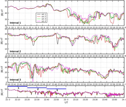
interest-ing structures are revealed. Figure 12 shows the FGM mag-netic field magnitude from the four Cluster spacecraft in the interval 22:00 to 24:00 UT. The first three panels show the data between 22:00–22:20 UT, 22:20–22:40 UT and 22:40– 23:00 UT, whilst the fourth panel summarises the Cluster FGM observations in the interval 22:00–24:00 UT. Again, the entry into the boundary later at 22:10 UT and the magne-topause crossing around 23:40 UT are both clearly seen. Fol-lowing the entry into the boundary layer (BL) at 22:10 UT, the Cluster spacecraft measure magnetic field variations with short correlation lengths; different spacecraft measuring dif-ferent field fluctuations. In agreement with the single space-craft data shown in Fig. 10, there is a transition into a less turbulent and more magnetosphere-like region within the BL (with longer correlation lengths) between 23:18 and 23:40 UT, perhaps as a result of outwards motion of the magnetopause and boundary layer moving Cluster closer to the magnetosphere. After the magnetopause crossing at 23:40 UT, the correlation between individual Cluster space-craft is again reduced, consistent with the Cluster spacespace-craft moving into the magnetosheath proper.

The fourth panel of Fig. 12 also highlights three particu-lar regions of interest, each of which are magnified in pan-els one, two and three. In the first panel, all four Cluster spacecraft see effectively the same magnetic field as they travel through the outer lobe towards the magnetopause un-til around 22:10 UT. At this time, the four Cluster spacecraft enter the magnetosheath boundary layer (BL), each space-craft entering the lower field magnitude region in the bound-ary layer at slightly different times. Spacecraft two (red) en-ters the BL first, with spacecraft one and three (black and green) crossing the BL next, followed by Cluster four (ma-genta). Looking again at the Cluster orbit configuration plot in Fig. 9, the ordering of the spacecraft entries into the BL can be understood on the basis of the orientation of the space-craft with respect to the expected model magnetopause ori-entation. Figure 9 shows that in the X − Y plane, Cluster 2 (red) is situated at highest GSE X position, and would be ex-pected to enter the BL first at this local time. Subsequent MP crossing would then be expected by Cluster 3, followed by Cluster 1 and 4. However, Cluster 1, 3 and 4 do not lie at the GSE Z position. In the northern lobe, the magnetopause will be inclined towards higher Z at lower Y . Based on the Cluster orientation in the Y Z plane, where Cluster 4 lies at the lowest position in Y and Z, we would expect Cluster 1 and 3 to cross the MP before Cluster 4, exactly as observed.

Given that the low shear entry into the BL at 22:10 UT is characterised by MVA field angles θbnwhich are close to

zero, the ordering of the spacecraft entries into the BL is also consistent with the hypothesis that the MVA normal from the 23:40 UT MP crossing also characterises the (presumably planar) geometry of the edge of the magnetosheath bound-ary layer. Hence we can conclude that the entry of Cluster into the magnetosheath BL at 22:10 UT can be explained by the motion of the edge of the locally planar BL across the spacecraft, whose normal lies close to the expected model magnetopause direction.

Examining the structure of the magnetosheath boundary layer between 22:10 UT and 23:00 UT shows that there are number of excursions of the Cluster spacecraft into regions characterised by low |B|. Some of the entries into regions of lower magnetic field magnitude are observed by the Clus-ter spacecraft in the same sequence as that observed at the 22:10 UT entry into the magnetosheath BL (and that of the 23:40 UT magnetopause crossing) consistent with the advec-tive motion of large scale approximately planar structures in the magnetosheath boundary layer across the spacecraft. For example, examining both Figs. 10 and 12, it is clear that, fol-lowing entry into the BL at 22:10 UT, Cluster enters a low

|B| region, the individual Cluster spacecraft maintaining

ap-proximately the same entry sequence as for the BL cross-ing at 22:10 UT before reachcross-ing the minima in |B| at around 22:13–22:14 UT. The subsequent motion back into a region of higher |B| broadly shows the reverse spacecraft ordering, although the signatures appear to be more complex. Other clear examples of entries into regions of low |B| with the same ordering can be seen beginning at around 22:23 UT, 22:36:30 UT, 22:43:30 UT and 22:49 UT, the minima in |B| observed by Cluster 3 being marked by green solid vertical lines in Fig. 10.

We believe that these regions of low |B| are observed by Cluster as a result of the advection of the magnetosheath boundary layer across the spacecraft, resulting in the sam-pling of regions of lower magnetic field which lie closer to the magnetopause, although probably not resulting in the crossing of the magnetopause itself. Examining the entries of the Cluster satellites into regions of low |B| in the boundary layer appears to suggest a possible 6–7 min quasiperiodic se-quence. There are minima in |B| around 22:13 UT, 22:24 UT, 22:31 UT, 22:38 UT, 22:44 UT and 22:56 UT (cf the green solid vertical lines in Fig. 10). As shown in Fig. 10, the de-crease in |B| is, in general, related to a dede-crease in magni-tude of both BXand BY. There is also some evidence that

this quasi-periodic series may continue with |B| and BX

de-creases also being observed around 23:02 UT, 23:08 UT and 23:16 UT. Interestingly, during the regions of low |B|, there is the suggestion from the bottom panel of Fig. 11 that these may also be accompanied by rotations of the MVA angle θbn

close to zero. This may be suggestive of motion of the Clus-ter satellites closer to the magnetopause within the BL.

The 6–7 min quasiperiodic sequence of entries into regions of low |B| between 22:13 UT and 22:56 UT does, however, appear to be interrupted by |B| dips missing at times around 22:18 UT and 22:50 UT. Interestingly, as shown in the four spacecraft data from Fig. 12, at 22:18 UT there is evidence of a classic nested partial entry into a region of lower |B|. Here, Cluster 4 does not enter the low |B| region, whilst Cluster 1 and 3 appear partially to enter a lower |B| region; Cluster 2 enters furthest into the low |B| region. This would be consistent with smaller amplitude inward motion of the magnetosheath boundary layer and hence only a partial en-try of the Cluster quartet into a region of lower |B|. This might be expected immediately following entry into the BL when the spacecraft remain close to the magnetosphere and

21: 00 21:30 22: 0 22:30 23: 0 23:30 24: 0 20 40 60 Bmag nT UT −20 0 20 40 Bx nT −20 0 20 By nT −20 0 20 Bz nT B L M P |B| dips

Fig. 10. GSE BZ, BY, BX (first

three panels), and |B| from Clus-ter 3 from 21:00 UT until 24:00 UT on 9 December 2000. Entry into the magnetosheath boundary layer (BL) at 22:10 UT and the magnetopause (MP) crossing around 23:40 UT are shown as red dashed lines, whilst excursions into regions of low |B| are indicated by green vertical lines in the final panel. See text for more details.

−150 −100 −50 0 50 100 150 200 250 300 350 −80 −60 −40 −20 0 20 40 60 80 φ θlat Analysis interval = 23:34 − 23:48 UT 21: 0 21:10 21:20 21:30 21:40 21:50 22: 0 22:10 22:20 22:30 22:40 22:50 23: 0 23:10 23:20 23:30 23:40 23:50 24: 0 −60 −40 −20 0 20 40 60 θbn n MVA = (0.63, 0.49, 0.60)

Fig. 11. (a) A scatter plot of the

GSE magnetic field angles observed by Cluster 2 from 23:34–23:48 UT (pink crosses), and a best fit curve corre-sponding to a planar fit to the data

(green curve) (top panel).

Overplot-ted in red is the curve corresponding to a plane derived from a minimum

variance analysis (nMVA)from the same

interval. (b) The magnetic angle out

of the minimum variance plane (θbn)

observed by Cluster 2 for the interval 21:00–24:00 UT on 9 December 2000 (bottom panel).

relatively far from the oscillating magnetopause. Certainly the observations in the interval 22:10–23:00 UT seem to be generally supportive of excurions into regions of increasingly lower |B| as Cluster travels deeper into the magnetosheath boundary layer. Similarly, at 22:49 UT there is evidence of sequential Cluster satellite motion into a slightly lower |B| region with the same ordering as the 22:10 UT entry into the BL. After 22:49 UT, as with the other entries into regions of low |B| in the quasi-periodic sequence, a clear decrease in BX is observed. However, in this case |B| does not

de-crease to such a low magnitude as that seen in the adjacent

|_{B| dips around 22:44 UT and 22:56 UT. This may be in part}

because the change in BXis partially offset by an increase in

BZ. Consequently, the observations from both 22:18 UT and

22:49 UT can still be interpretted as being supportive of fill-ing in the missfill-ing entries in the hypothesised 6–7 min quasi-periodic sequence.

This quasi-periodic motion of the magnetpause and boundary layers is consistent with that expected for a global mode of the magnetosphere, this global mode perhaps being excited by the development of the KHI on the dusk flank. For this explanation to be correct the KHI is required to have a wavelength which is much longer than both the Clus-ter spacecraft separation and the oscillatory displacement of the magnetopause, so that the local orientation of the mag-netopause and boundary layer is approximately the same at each spacecraft and relatively close to the expected model MP orientation. As pointed out above, for crossings from the

22: 0 22:10 22:20 22:30 22:40 22:50 23: 0 23:10 23:20 23:30 23:40 23:50 24: 0 0 50 |B| nT UT 22:40 22:41 22:42 22:43 22:44 22:45 22:46 22:47 22:48 22:49 22:50 22:51 22:52 22:53 22:54 22:55 22:56 22:57 22:58 22:59 23: 00 10 20 30 40 5022:20 22:21 22:22 22:23 22:24 22:25 22:26 22:27 22:28 22:29 22:30 22:31 22:32 22:33 22:34 22:35 22:36 22:37 22:38 22:39 22:40 0 10 20 30 40 5022: 0 22: 1 22: 2 22: 3 22: 4 22: 5 22: 6 22: 7 22: 8 22: 9 22:10 22:11 22:12 22:13 22:14 22:15 22:16 22:17 22:18 22:19 22:20 30 35 40 45 50 s/c 1 s/c 2 s/c 3 s/c 4 Interval 1 Interval 2 Interval 3 1 |B| nT 3 |B| nT 2 |B| nT

Fig. 12. Cluster four spacecraft measurements of |B| in the intervals 22:00–22:20 UT (first panel), 22:20– 22:40 UT (second panel) and 22:40– 23:00 UT (third panel). The final panel shows a summary of the interval 22:00– 24:00 UT; blue horizontal bars indicate the intervals expanded in the three pan-els above.

0.00 1.00 2.00 3.00 4.00 5.00 6.00 7.00 8.00

Day 345, 2000 : H Component : Unfiltered 194.0nT NAL 264nT LYR 450nT HOP 522nT BJN 420nT AND 402nT TRO 356nT ABK 368nT KIL 360nT MAS 344nT KEV 314nT KIR 310nT MUO 324nT PEL 318nT SOD 134.0nT FAR 176.0nT NOR 132.0nT OUJ 51.5nT HAN 49.5nT NUR 43.5nT UPS 42.0nT BOR 27.5nT YOR 0.00 1.00 2.00 3.00 4.00 5.00 6.00 7.00 8.00

Day 345, 2000 : D Component : Unfiltered 164.0nT NAL 194.0nT LYR 270nT HOP 318nT BJN 112.0nT AND 134.0nT TRO 100.0nT ABK 104.0nT KIL 138.0nT MAS 108.0nT KEV 88.0nT KIR 99.5nT MUO 81.5nT PEL 85.5nT SOD 64.0nT FAR 51.5nT NOR 55.5nT OUJ 45.5nT HAN 34.5nT NUR 31.5nT UPS 46.5nT BOR 33.5nT YOR

Fig. 13. Stacked H -component (a) and D-component (b) magnetograms from selected IMAGE and SAMNET magnetometer stations

between 00:00 UT and 08:00 UT on 10 December 2000. Each magnetogram is independently scaled, the amplitude being indicated by the bars on the left hand side of each figure.

magnetosphere into the magnetosheath, the KH would be ex-pected to rotate the normal to point slightly sunwards of the model MP normal (cf. Fairfield et al., 2000); we discuss this further below.

There are also some partial entries of the Cluster spacecraft into lower |B| regions which do not fit the quasi-periodic sequence, such as that seen by Cluster 1 at 22:28:30 UT or the partially nested structure seen at 22:41:30 UT. However, these two cases may be the result of motion of the magnetopause due to changes in upstream ram pressure or result from local scale structures in the mag-netosheath, rather than the development of long down-tail wavelength KHI. Indeed, both of these cases appear to repre-sent situations where the Cluster satellites sample smaller |B| excursions than those adjacent |B| dips which do fit with the quasi-periodic sequence. Moreover, the observations from 22:28:30 UT show a case where Cluster 1 clearly samples the lowest |B| of all four Cluster satellites. Since Clus-ter 1 lies at the highest Z, this is consistent with the mag-netopause and boundary layer moving towards lower Z and flattening the magnetosphere and magnetosheath compared to both the model magnetopause shape and the normals in-ferred from the 22:10 UT and 23:40 UT BL and MP cross-ings. This would leave Cluster 1 sampling lower |B| as it “pokes out” further into the boundary layer as compared to the other Cluster satellites and could be consistent with dis-tortion of the magnetopause and boundary layer on smaller spatial scales.

If the Cluster spacecraft are seeing periodic entries into low |B| regions as a result of the periodic motion of an ap-proximately planar magnetosheath boundary layer and mag-netopause, due to the action of the KHI, one might expect that there would be similar quasi-periodic entries into re-gions of higher |B| at the maxima of the outwards motion of the magnetopause. There are examples of transitions with exactly the reverse ordering to that observed for the BL en-try at 22:10 UT (Cluster 4, then Cluster 1,3, and then Clus-ter 2), presumably as a result of the global outwards mo-tion of the magnetopause and boundary layer. Indeed, as mentioned above, following the |B| dip at 22:13 UT there is clear outward motion with the expected ordering begin-ning at 22:14 UT. Similarly, the nested signature at 22:18 UT suggests clear inward then outward motion of the bound-ary layer. In a similar fashion, there is evidence of outward motion around 22:24:30 UT (following the inward motion at 22:23 UT); mid-way between the |B| dip at 22:31 UT and that at 22:38 UT there is another example of outward motion beginning at 22:34 UT. However, in this latter instance, the ordering of Cluster 1 and 2 is reversed from that expected for the motion of a planar boundary aligned with the mag-netopause. This motion is immediately followed by what appears to be inward motion at 22:35 UT, where the Clus-ter spacecraft measurements are again ordered by the ex-pected MP orientation. In general, the spacecraft ordering for outward motion of the boundary layer appears to be much more complicated than that for the inward motion. Often, for the outward motion of the boundary layer, the ordering seen

by Cluster does not match that expected from the outward motion of planar structures whose orientation is determined by model magnetopause orientation. This suggests that the orientation of the magnetopause and magnetosheath bound-ary layer may differ between inbound and outbound motion. This could be explained by the development of KH vortex structures on the MP and in the BL; we discuss this further below.

In general the Cluster observations are consistent with quasi-periodic inward and outward motion of the magne-topause and magnetosheath boundary layer across the Clus-ter quartet. This quasi-periodic motion is what would be ex-pected from a global magnetospheric oscillation such as a magnetospheric waveguide mode. Indeed, since the periodic magnetosheath motion has the same period as the ULF waves on the ground in Canadian sector, LT conjugate to Cluster (see Fig. 1), there is the strong suggestion that the motion of the magnetopause may have been related to driving the FLRs seen on the ground. It is possible that the development of a long wavelength KHI on the dusk flank caused the periodic global motion of the magnetosheath boundary layer across the Cluster quartet and that this KHI was the energy source for the large amplitude ULF waves seen on the ground. It should be noted, however, that any global compressional os-cillations of the magnetosphere would be expected to cause inward and outward motion of the magnetopause. We dis-cuss the possible solar wind energy sources for these global oscillations further below.

3.3 Ground-based dawn sector observations

During the interval 00:00–08:00 UT, on 10 December 2000 (DOY 345), ground-based instrumentation in the European sector also observed very large amplitude ULF waves as the Earth’s rotation moved it into the dawn flank. Figure 13 shows the unfiltered H (a) and D (b) component magnetome-ter data from selected stations of the IMAGE and SAMNET magnetometer arrays (see Fig. 1 and Table 2 for details of the station locations). As can be clearly seen, very large amplitude ULF waves are prevalent throughout this inter-val across the whole European sector, with particularly clear wave packets between 00:45–02:00 UT, 03:30–04:00 UT and 04:45–06:10 UT.

Figure 14 shows the stacked H -component power spec-trum, filtered between 100 s and 600 s, for these IMAGE and SAMNET magnetometer stations between 00:45–02:15 UT. A sharp spectral peak, whose frequency is independent of latitude, can be seen at around 3.2 mHz, with a smaller sub-sidiary latitude independent peak at around 4.5 mHz (this lat-ter peak being less clear on the more weslat-terly SAMNET sta-tions during this interval).

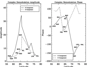
In Fig. 15 we show the results from a complex demod-ulation analysis of the 3.2 mHz spectral component from a latitudinal chain of selected magnetometer stations from the IMAGE array (bandpassed between 3.0 mHz and 3.3 mHz and taking an average of the two maximum H amplitude de-modulates from around 01:50 UT). Similar to the ULF waves

0 1 2 3 4 5 6 7 Frequency (mHz)

POWER (Arbitrary Units, independently scaled)

NAL

0.0 340.565

Day 345, 0 0:45 for 90 minutes

H Component : Filtered 600 to 100 s : Smoothed over 1 Estimates

LYR 0.0 491.763 HOP 0.0 465.78 BJN 0.0 495.26 AND 0.0 733.042 TRO 0.0 691.664 ABK 0.0 765.328 KIL 0.0 807.266 MAS 0.0 798.726 KEV 0.0 689.935 KIR 0.0 719.244 MUO 0.0 803.828 PEL 0.0 782.675 SOD 0.0 777.497 FAR 0.0 868.689 NOR 0.0 801.26 OUJ 0 500 HAN 0.0 841.652 NUR 0.0 965.53 UPS 0 1000 BOR 0.0 816.356 YOR 0.0

674.283 Fig. 14. Stacked H -component power

spectra for the selected SAMNET and IMAGE magnetometer stations shown in Fig 14. Each power spectra is inde-pendently scaled.

seen by CANOPUS on the dusk flank, the IMAGE mag-netometers show these dawn flank waves to be dominanted by the H -component on the ground as expected for a domi-nantly toroidal wave in the magnetosphere. Again, the FLR characteristic is verified by the 180◦latitudinal phase change seen in the H -component. For this wave packet, the D-component also shows a latitudinal peak; however, there is a smaller phase change across the array in this component.

We can also estimate the azimuthal wavenumber of the waves by examining the phase changes at the longitudes lo-cal to the latitudinal chain of magnetometer stations shown in Fig. 15. Examining the phases from the complex demod-ulation analysis from Fig. 15 and using the D-component to minimise latitudinal phase changes, results in an m-value of

∼ −8.0 ± 1.4 from stations PEL and SOD. Closer to the resonance, the longitudinal chain KIL-MAS-KEV produces more variable phase estimates; however they are consistent with westward phase propagation with m<∼10.

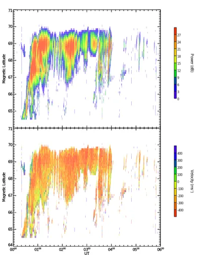
The clear ULF wave activity, seen by the IMAGE and SAMNET magnetometers, was also observed by the STARE VHF radar in the European sector. Figure 16 shows the radar back scatter power (top panel) and flow velocity (bot-tom panel) from beam 2 of the STARE Norway radar be-tween 00:00 UT and 06:00 UT on 9 December 2000. In the backscatter power returns, very clear wave activity in the Pc5 band can be seen between 01:30–02:00 UT and between 03:30–04:00 UT, with smaller amplitude activity being ob-served throughout the interval from 00:30–04:00 UT. The wave activity is seen clearly in both the backscatter power and velocities between around 67 and 70 degrees geomag-netic, with evidence of the polewards phase propagation ex-pected for a low-m FLR (e.g. Wright and Allan, 1996a).

To examine the wave characteristics in more detail, we show in the top panel of Fig. 17 the backscatter power from selected range gates from beam 2. In this plot, very clear sinusoidal backscatter power oscillations are apparent,

par-Fig. 15. Complex demodulation H and D-component amplitude

and phase for the 3.2 mHz wave (average of 2 demodulates centred around 01:50 UT).

ticularly between 01:20–02:00 UT and 03:30–04:00 UT. The second panel in Fig. 17 shows the velocities seen by the CUT-LASS Hankasalmi radar beam 5, close to the location of the STARE backscatter power returns.

At the beginning (before 00:30 UT) and end (after 04:00 UT) of the interval shown in Fig. 16 there is no STARE radar backscatter, due to a lack of scattering irregularities resulting from the low ambient electric field (see e.g. Wal-dock et al., 1985). The VHF radar backscatter, seen by the STARE system in the centre of the interval, corresponds to an interval of enhanced ionospheric convection, as can be seen from the north-western pointing beam of the CUTLASS Hankasalmi radar in the bottom panel of Fig. 17 (see also Greenwald et al., 1995). The enhanced electric fields will produce backscatter through the two-stream instability (see e.g. Fejer and Kelly, 1980). The observed phase velocity of such backscatter is not a direct measurement of the line of sight component of the E × B velocity but is limited to the acoustic speed of the E-region ionosphere, although this itself increases non-linearly with the E × B velocity (Robinson, 1986). The enhanced convection electric field is then modulated by the ULF wave electric field, such that in-complete data coverage is available throughout the wave cy-cle, complicating any analysis of the wave (Yeoman et al., 1992). However the observed Doppler velocities are unidi-rectional and the backscatter intensity, which itself increases with E × B velocity, will thus provide a good proxy for the ULF wave amplitude (see Yeoman et al., 1990b; Shand et al., 1996).

To examine the properties of the ULF waves seen by STARE, Fig. 18 shows the unfiltered power spectrum of the backscatter power from beam 2, range gate 38, between 01:30–02:00 UT. A clear broad spectral peak, centred on 2.7 mHz, can be seen, in good agreement with the magne-tometer observations presented in Fig. 14. In Fig. 19 we show the latitudinal amplitude and phase variation of the

2.7 mHz component from STARE beam 2 for range gates 28, 30, 32, 34, 36, 38, 40 (cf., the top panel of Fig. 17). A clear latitudinal amplitude maximum, at around 68.7◦

geo-magnetic, is seen with a phase change of around 50◦between 67.8 and 69.1◦.

Clearly, there is excellent agreement between the wave ac-tivity seen by STARE and by the magnetometers. Both see a clear ULF wave with frequency close to 3.2 mHz (note that the STARE radar spectrum in Fig. 18 has limited fre-quency resolution due to the analysis of only 30 min of data). The STARE data shows that the power in spectral peak at 2.7 mHz demonstrates both the amplitude maxima and phase change expected from a FLR. Comparing Figs. 19 and 15, we see that the STARE inferred resonant latitude lies in the gap of magnetometer coverage between MAS and BJN (66– 71◦_{geomagnetic). The resonant latitudes inferred from the}

IMAGE and STARE data appear to be entirely consistent with the limited latitudinal extent of the STARE backscat-ter, revealing part of the expected 180◦phase change which is seen over a wider latitudinal range by the magnetometers. Previous observations of Pc5 ULF waves have also placed the resonant field line of waves around 3 mHz frequency be-tween the Scandinavian mainland and BJN station (c.f., the 2.6 and 3.7 mHz FLRs presented in Fig. 8 of Mathie and Mann, 2000).

We can also estimate the azimuthal wavenumber of the waves using the STARE observations in this interval. Since the STARE radar measures variations along the radar line of sight, calculating the m-values with STARE requires a care-ful consideration of the geometry of the differing look direc-tions from beam to beam, which can influence the inferred

m-values especially if the waves are not linearly polarised. Low-m FLRs are, in general, elliptically polarised at reso-nance and this can cause the radar beam geometry to influ-ence radar inferred m (see e.g. Ziesolleck et al., 1998). The STARE data in the interval 01:30–02:00 UT suggest west-wards phase propagation with an m-value ∼ 4. This is con-sistent with the magnetometer estimates and, with a FLR be-ing driven by a tailwards propagatbe-ing source such as a mag-netospheric waveguide mode, in the morning local-time sec-tor. Moreover, this suggests that the STARE latitudinal phase profile shown in Fig. 19 is not significantly contaminated by the 3◦of longitude covered by the latitudinal range.

Returning to Fig. 13, we can see that large amplitude ULF wave activity continues thoughout the morning sector. Sev-eral other large amplitude wavepackets are apparent in both the H - and D-components, the H -component being dom-inant in each wavepacket with the two wave packets be-tween 03:30–04:00 UT and 04:45–06:10 UT being particu-larly clear. Amplitude and phase analysis of the 03:30– 04:00 UT wave packet show that there is a clear spectral peak at around 2.5 mHz however, the behaviour of the amplitude and phase at this frequency during this interval is compli-cated by the large amplitude impulsive signature at around 03:52 UT. This feature is clearly related to a poleward mov-ing arc seen by the all-sky-cameras (ASC) of the MIRACLE network (not shown). The ASC camera, the magnetometer,

65 66 67 68 69 70 71 Magnetic Latitude 65 66 67 68 69 70 71 Magnetic Latitude 0 3 6 9 12 15 18 21 24 27 Power (dB) 0000 ₀₁00 ₀₂00 ₀₃00 ₀₄00 ₀₅00 ₀₆00 UT 64 65 66 67 68 69 70 71 Magnetic Latitude 0000 ₀₁00 ₀₂00 ₀₃00 ₀₄00 ₀₅00 ₀₆00 UT 64 65 66 67 68 69 70 71 Magnetic Latitude -400 -300 -200 -100 0 100 200 300 400 Velocity (ms -1 )

STARE PARAMETER PLOT

Fig. 16. Backscatter power (top panel)

and velocity (lower panel) for the STARE Norway radar, beam 2, between 00:00 UT and 06:00 UT on 10 Decem-ber 2000.

and the STARE data are all consistent with the interpretation of a poleward propagating upward FAC at around 03:52 UT. Other oscillations earlier in this wavepacket also show the signatures of upwards FAC; however they do not appear to have optical counterparts. Consequently, it is difficult to de-termine whether this arc is related to the pulsation activity which exists throughout the 03:30–04:00 UT interval or is driven by a separate propagating field aligned current (FAC) system which crosses the MIRACLE network at the same time. The wavepacket between 04:45–06:10 UT seems to represent a more continous wavetrain and can be seen to con-tain a number of discrete spectral components. Figure 20 shows the unfiltered H -component power spectrum between 04:30–05:45 UT; clear latitude-independent discrete spectral peaks are apparent at around 1.9, 2.7, 3.7, and 4.6 mHz. Lati-tudinal amplitude maxima and phase changes consistent with the excitation of FLRs are seen for each spectral compo-nent (not shown). Figure 21 shows the frequencies and the corresponding modulus of the m-values for the wavepack-ets seen in Fig. 13 for the two discrete frequencies seen between 01:30–02:00 UT (cf. Fig. 14) and the four dis-crete frequencies seen between 04:45–06:10 UT (cf Fig. 20).

m-values were calculated using the D-component from the SOD-PEL station pair, to minimise the effects of latitudinal phase changes which dominate near the resonance and have more influence in the H - rather than the D-component. The

m-values, shown in Fig. 21, were all measured to be nega-tive (westward) consistent with tailward phase propagation in the morning sector; however, the figure shows the mod-ulus of m for clarity. The frequency components from the earlier wave packet are marked with an x-symbol in Fig. 21, the error bars in frequency and m-value are calculated on the basis of the bandwidth of the complex demodulation analy-sis used to isolate each spectral component and the standard deviation in the m-value estimates taken over the maximum

H-component amplitude demodulates, respectively. Both wavepackets suggest that there might be an almost linear re-lationship between frequency and m-value; the dot-dashed lines show an approximate best-fit line through the origin and the data points. Hence, we can estimate the azimuthal phase speed of these wavepackets in the ionosphere, using the relationship vphI = 2π REcos 3f/m where RE is the

Earths radius, 3 is the latitude of the observation and f is the wave frequency. This results in (westward) ionospheric

STARE/SuperDARN Hankasalmi

(b) Hankasalmi beam 5 velocity, ranges 18 20 22

) (increment = 400)

(a) STARE beam 2 power, ranges 30 32 34 36 38 40

0000 ₀₁00 ₀₂00 ₀₃00 ₀₄00 ₀₅00 ₀₆00 UT 50 100 150 Power (dB) (increment = 30)

Fig. 17. Stacked STARE Norway radar backscatter power from

beam 2 and range gates 30, 32, 34, 36, 38 and 40 (a), and stacked SuperDARN Hankasalmi radar beam 5 velocity from range gates 18, 20 and 22, between 00:00 UT and 06:00 UT on 10 December 2000 (b).

STARE PARAMETER PLOT

0 5 10 15 Spectral Power 0 2 4 6 8 10 Frequency (mHz)

Fig. 18. Power spectrum from STARE Norway beam 2, range gate

38, between 01:30 UT and 02:00 UT.

0 5 10 15 20

Power (Arb. Units) 67.5 68.0 68.5 69.0 69.5 Magnetic latitude 50 100 150 Phase (degrees)

Fig. 19. Amplitude and phase of the 2.7 mHz spectral component

observed by the STARE Norway radar beam 2 in range gates 28, 30, 32, 34, 36, 38, 40, in the interval 01:30–02:00 UT on 10 December 2000.

phase speeds of 6.7 km/s and 12.0 km/s for each of the two wavepackets respectively, where we have assumed a latitude of 66◦close to the stations recording maximum amplitudes. These phase speeds compare well with previous estimates of FLR common azimuthal phase speeds as presented, for ex-ample, by Mathie and Mann (2000) (e.g. their Fig. 4), and are consistent with the downtail (westward) phase propaga-tion expected in the morning sector.

4 Discussion

The characteristics of the FLRs reported here are in good agreement with those recently presented by previous authors who have attributed the FLR excitation to waveguide modes (e.g. Mathie et al., 1999). Recent theoretical work by Mann et al. (1999) (see also Mills et al., 1999) has shown that the Kelvin-Helmholtz instability can excite body type waveg-uide modes, in addition to the standard KH surface waves. Later work by Mills and Wright (1999) and Mann and Wright (1999) (see also Wright and Rickard, 1995) has shown that multiple FLRs excited by several radial waveguide mode har-monics will be expected to possess the same azimuthal phase speed. Observational evidence (e.g. Mathie and Mann, 2000) has now placed this hypothesis on a firmer footing by

show-0 1 2 3 4 5 6 7 Frequency (mHz)

POWER (Arbitrary Units, independently scaled)

NAL

0 500

Day 345,2000 4:30 for 105 minutes H Component : Unfiltered : Smoothed over 1 Estimates

LYR 0 200 TRO 0 200 AND 0 200 ABK 0 200 MAS 0 200 KIL 0 200 KEV 0 200 MUO 0 200 PEL 0 200 SOD 0 200 OUJ 0 200 HAN 0.0 195.476 NUR 0 200 UPS 0 200

Fig. 20. Unfiltered H -component power spectra from selected IMAGE magnetometer stations between 04:30– 05:45 UT. Clear latitude independent spectral peaks are apparent at around 1.9, 2.7, 3.7 and 4.6 mHz.

ing clearly how common azimuthal phase speed FLRs can be driven during fast solar wind speed intervals. According to the theory of Mann et al. (1999), body waveguide modes (in addition to the usual surface modes) can be energised by the KHI once the magnetosheath flow speed exceeds a crit-ical speed ∼ 500 kms−1 (the exact critical speed depends upon variations in the sound and Alfv´en speeds and the mag-netic field across the magnetopause). The theory is in excel-lent agreement with the observations of Engebretson et al. (1998) (see also Mathie and Mann, 2001) who showed that ULF wave power in the morning side increases significantly when the solar wind speed >∼500 kms−1. Statistical

stud-ies of the diurnal variation of Pc5 ULF wave power show that it is strongly peaked in the morning local time sector. As discussed by Mann and Wright (1999), stabilising IMF magnetic field tension in the dusk local time sector is usually cited as a likely reason for the dawn-dusk flank asymmetry (see Lee and Olson, 1980). Further, and as shown by Mann

et al. (1999), the KHI acts through the propagation of distur-bances against the background flow. In the magnetospheric frame, the down-tail phase speed of waves driven by the KHI only occurs because they are advected downstream by the flow. This should result in azimuthal phase speeds, vph, for

KH driven FLRs which are < U .

In the observations we have presented here, there is clear observational evidence for the excitation of large amplitude Pc5 FLRs on both the dawn and dusk flanks during an in-terval of fast solar wind speed. Figure 21 shows that the multiple frequency FLRs observed on the dawn flank in the intervals between 01:30–02:00 UT and 04:45–06:10 UT had common ionospheric azimuthal phase speeds of 6.7 kms−1 and 12.0 kms−1, respectively. Assuming an equatorial mag-netopause standoff distance of 10 RE, produces estimates of

the magnetopause phase speeds of around 170 kms−1 and 300 kms−1, respectively. These phase speeds are likely to be less than U at the local times of the measurements,

espe-Fig. 21. Wave frequency and m-values from the two discrete

fre-quencies in the wavepacket between 01:30–02:00 UT (x-symbols) and the four discrete frequencies in the wavepacket between 04:45– 06:10 UT. Dot-dashed lines represent lines of approximate best fit through the origin in each case. See text for more details.

cially given that on the flanks the magnetosheath speed ap-proaches the upstream solar wind speed (e.g. Spreiter and Stahara, 1980). Consequently, the low, common azimuthal phase speed property of the FLRs on the dawn flank pro-vides excellent evidence that the KHI was responsible for energising waveguide modes which themselves drive large amplitude FLRs on the dawn flank (cf. Mann and Wright, 1999).

On the dusk flank, however, multiple frequency FLRs were not recorded in the interval studied (between 00:00– 00:40 UT). Using the m-value estimated from the D-component at the ISL and MCM stations (3 ≈ 64.5◦), for a 6 min period wave, results in a significantly faster iono-spheric azimuthal phase speed of around 28 kms−1. Map-ping this speed to a model magnetopause at 10 REproduces a

magnetopause phase speed ∼ 650 kms−1, very similar to the upstream solar wind speed. As discussed above, the fastest growing KHI driven modes will, in general, be expected to drive FLRs with phase speeds somewhat lower than the local sheath speed (see e.g. Mills and Wright, 1999, their Fig. 11); however, more slowly growing modes might be excited with speeds closer to U . Hence, on the basis of the phase speed, we cannot unambigously determine whether the dusk flank FLR was driven by a KH unstable waveguide mode. In-deed, according to Mann and Wright (1999), a phase speed

vph∼Umay be more suggestive of a magnetopause running

pulse driver than the development of the KHI.

Very recently, Sarafopoulos et al. (2001) have presented ground-based magnetometer observations of large amplitude ULF waves on both the dawn and dusk flanks during an interval of fast solar wind speed. They also proposed the KHI as the mechanism which energised the pulsations. De-spite having no in situ measurements local to the

magne-topause, Sarafopoulos et al. (2001) observed periodic vari-ations in the > 38 keV electron channel on Geotail in the magnetosheath. These authors argued that magnetopause motion provided a periodic magnetic connectivity between Geotail and the oscillating magnetopause. The electron sig-natures occurred during intervals of magnetic connectivity to the magnetopause, providing a remote signature of periodic magnetopause oscillations on the dawn flank.

In this study, we are fortunate to have in-situ Cluster data from the dusk flank which can be used to examine the mo-tion and orientamo-tion of the magnetopause and boundary lay-ers. The Cluster data can be used to test the hypothesis that the ground pulsations are related to global waveguide modes with corresponding periodic magnetopause motion, perhaps due to the excitation of the KHI. During the interval immediately preceding the observations of the largest am-plitude ULF waves on the ground in the Canadian sector (00:00–00:40 UT), the Cluster satellites were following an outbound trajectory through the high latitude dusk lobe and into the magnetosheath, crossing the MP at 23:40 UT. Fol-lowing the entry into the magnetosheath BL, at 22:10 UT, Cluster repeatedly and quasi-periodically sampled regions of low |B| in the magnetosheath boundary layer (BL) be-tween 22:24–22:56 UT (and possibly longer until around 23:16 UT). While the location of the Cluster quartet in rela-tion to the equilibrium posirela-tion of the magnetopause was not such that motion of the magnetopause and BL caused Clus-ter to repeatedly cross the magnetopause, the ClusClus-ter obser-vations were consistent with the quasi-periodic motion ad-vecting a locally planar magnetosheath BL across the satel-lites. This might have resulted in the repeated observation of regions of lower magnetic field magnitude as the satellites repeatedly made observations closer to the magnetopause.

As discussed by Fairfield et al. (2000) (see also Otto and Fairfield, 2000, and references therein), for MP crossings which move satellites into the magnetosheath from the mag-netosphere, the action of the KHI might be expected to ro-tate the MVA magnetopause normal in a sunward direction as compared to the expected model MP orientation. While the periodic motion in the magnetosheath boundary layer did not generate multiple magnetopause crossings, when Clus-ter crossed the MP at 23:40 UT a slight sunward rotation of the normal was observed which may be consistent with the action of the KH in the manner described by Fairfield et al. (2000).

Interestingly, for the quasi-periodic inward motion of the magnetosheath BL (which moves the Cluster satellites fur-ther towards the magnetopause) the 4 satellite timings are consistent with the motion of a locally planar structure which is approximately aligned with the expected local MP orien-tation. If the flank waveguide has a magnetopause stand-off distance of 10 RE, typical of waveguide mode driven

FLRs with azimuthal wavenumbers m ∼ 2 − 10 will have downtail (azimuthal) wavelengths ∼ 6 − 31 RE. These

wavelengths are very much larger than likely ampitudes of magnetopause displacement due to the KHI. Consequently, the angular distortion of the magnetopause normal detected