HAL Id: hal-01715092
https://hal.archives-ouvertes.fr/hal-01715092
Submitted on 23 Feb 2018
HAL is a multi-disciplinary open access
archive for the deposit and dissemination of
sci-entific research documents, whether they are
pub-lished or not. The documents may come from
teaching and research institutions in France or
abroad, or from public or private research centers.
L’archive ouverte pluridisciplinaire HAL, est
destinée au dépôt et à la diffusion de documents
scientifiques de niveau recherche, publiés ou non,
émanant des établissements d’enseignement et de
recherche français ou étrangers, des laboratoires
publics ou privés.
Distributed under a Creative Commons Attribution - NonCommercial - ShareAlike| 4.0
International License
criteria control drained soil liquefaction
Cécile Clément, Renaud Toussaint, Menka Stojanova, Einat Aharonov, C.
Clement
To cite this version:
Cécile Clément, Renaud Toussaint, Menka Stojanova, Einat Aharonov, C. Clement. Sinking during
earthquakes: Critical acceleration criteria control drained soil liquefaction. Physical Review E ,
Amer-ican Physical Society (APS), 2018, 97 (2), pp.022905. �10.1103/PhysRevE.97.022905�. �hal-01715092�
liquefaction
C. Clément1, R. Toussaint1,2,∗ M. Stojanova3,1, and E. Aharonov4
1
Institut de physique du globe de Strasbourg, Université de Strasbourg, CNRS, UMR 7516, 67084 Strasbourg Cedex, France.
2
PoreLab, Dept of Physics, University of Oslo, Norway.
3
Institut Lumière Matière, Université Lyon 1, CNRS, UMR 5586,
69361 Lyon Cedex 07, France.
4
Hebrew University of Jerusalem, Israel (Dated: February 23, 2018)
PACS numbers: 62.20.Mk, 46.50.+a, 81.40.Np, 68.35.Ct
ABSTRACT
This article focuses on liquefaction of saturated gran-ular soils, triggered by earthquakes. Liquefaction is de-fined here as the transition from a rigid state, in which the granular soil layer supports structures placed on its surface, to a fluid-like state, in which structures placed initially on the surface sink to their isostatic depth within the granular layer. We suggest a simple theoretical model for soil liquefaction and show that buoyancy caused by the presence of water inside a granular medium has a dramatic influence on the stability of an intruder resting at the surface of the medium. We confirm this hypothesis by comparison with laboratory experiments and Discrete Elements numerical simulations. The external excitation representing ground motion during earthquakes is simu-lated via horizontal sinusoidal oscillations of controlled frequency and amplitude. In the experiments, we use particles only slightly denser than water, which as pre-dicted theoretically, increases the effect of liquefaction and allows clear depth-of-sinking measurements. In the simulations, a micromechanical model simulates grains using molecular dynamics with friction between neigh-bours. The effect of the fluid is captured by taking into account buoyancy effects on the grains when they are im-mersed. We show that the motion of an intruder inside a granular medium is mainly dependent on the peak ac-celeration of the ground motion, and establish a phase diagram for the conditions under which liquefaction hap-pens, depending on the soil bulk density, friction prop-erties, presence of water, and on the peak acceleration of the imposed large-scale soil vibrations. We establish that in liquefaction conditions, most cases relax towards an equilibrium position following an exponential in time. We also show that the equilibrium position itself, for most liquefaction regimes, corresponds to the isostatic equilib-rium of the intruder inside a medium of effective density. The characteristic time to relaxation is shown to be es-sentially a function of the peak ground velocity.
∗renaud.toussaint@unistra.fr
INTRODUCTION
Under usual conditions, natural and artificial soils (used as geotechnical foundations or construction ma-terials) support the weight of infrastructure placed on their surface, and the stresses exerted on their surface are transmitted to the underlying grains along force chains [1]. However contacts between grains may be weakened during shaking, and/or by addition of a liquid phase, which in general exerts an additional fluid pressure on the grains. When these contacts break or slide, the sys-tem is not stable anymore, so that the granular medium loses its ability to support shear stress and flows as a liq-uid, which is referred to as liquefaction [2]. In such cases debris flows, avalanches, quicksands or liquefaction can occur. Buildings on liquefied soils may sink or tilt, and pipelines are displaced or float to the surface. All of the above phenomena may lead to significant damage.
In this paper we focus on soil liquefaction associated with earthquakes [2–4]. Some areas are well known to be prone to soil liquefaction, like the New Madrid Seis-mic Zone in the central United States or Mexico city in Mexico [2, 5]. The last main earthquakes which have been followed by severe liquefaction effects - listed in [4] - are the 1964 Alaska Earthquake, magnitude Mw 9.2 [6], the 1964 Niigata Earthquake, magnitude Mw 7.5 [7, 8], Japan, and the 2011 Christchurch Earthquake, magni-tude Mw 6.3 [9], New-Zealand.
Liquefaction was historically first explained by Terza-ghi [10], relating liquefaction occurrence to the effective stress in the material. Further geotechnical work [11, 12] improved the principe of Terzaghi in order to explain as many liquefaction cases as possible. The current under-standing of liquefaction, which underlies the construction principles for foundations and roads, can be summed up as follows: During earthquakes, seismic waves disturb the grain-grain contacts, and some weight initially car-ried by the sediments are then shifted to the interstitial pore water [2]. The consolidation of the saturated sed-iment occurs in effectively undrained conditions (due to the short timescale of earthquakes), and pore pressure builds up as the granular pack compacts. As a result,
the effective stress carried by the sediments decreases. If the pore pressure rises more, the solid weight can be entirely borne by pore water and the sediments become fluid-like, i.e. they cannot sustain shear stress in a static configuration. This accepted mechanism thus assumes that the granular media must lose its strength completely to produce liquefied behavior.
The above-described pore-pressure theory of earthquake-induced soil liquefaction and its recent advances indeed explain many natural instances of observed liquefaction [12–14], yet it fails to explain many other field observations of earthquake-induced liquefaction. Examples of types of field occurrences of liquefaction that are not explained by the pore-pressure theory [15] include far-field liquefaction triggered at low energy density [16, 17], liquefaction under fully drained conditions [18–20], repeated liquefaction [21] and liquefaction in pre-compacted soils [22].
In fact, elevated pore-pressure is not the only path for granular material liquefaction. The phenomenon of solid-liquid transition of granular materials is known in a more general framework as fluidisation. Fluidisation of a gran-ular medium occurs when an initially rigid medium looses its cohesion and starts behaving like a fluid. One of its most famous examples is quicksand - a granular medium which can support a body on its surface until the said body is not moving, whereas if it is moving, the body sinks into the quicksand [23, 24].
A compact, dense granular medium at rest behaves like a solid. The grains experience friction due to the normal stress they apply to each other, traditionally coming from the gravitational loading. The friction enables the grains to resist external forces without flowing [25] and sustain weight by redistributing it along force chains [1]. The im-portance of normal stresses for the rigidity of a granular medium can be illustrated with some recent penetration experiments. Lohse et al. in [26] and Brizinski et al. in [27] used a homogeneous air injection to loosen the gran-ular medium and unload some of the gravitational force on grains. After the injection was stopped, the granu-lar medium could not carry the weight it was carrying before, and any objects placed on its surface sank. In a more extreme situation, where the grains are loose and also have a very low density (expanded polystyrene), the penetration of the intruder is infinite, just like the pen-etration of a dense object in a liquid [28]. The external energy required for fluidisation can be of different nature. It can come, for example, from gravity forces [29–31], shear stress [32], vibrations [24, 33–36] or the flow of an interstitial fluid [37, 38], and produce granular flows that can exhibit fluid-like behavior such as buoyancy [34] or anti-buoyancy [39] force, waves on their surface [33, 40], flow instabilities [41–46] and size segregation [35, 36].
Granular media start to behave as fluids when global contact sliding initiates throughout the media. The force needed to initiate sliding depends on the strength of the grain contacts - for an easy fluidisation, one needs to un-load some of the normal stress, hence reducing the fric-tion forces. For example, the shear stress necessary to
make a granular layer flow decreases when the granular medium is vibrated [47], the vibrations weakening the granular contacts. The presence of an interstitial fluid can play a similar role. When the grains are immersed, the effective normal stress they are subjected to is low-ered by the pore pressure of the fluid, hence reducing the friction forces between grains. If the pore pressure is high enough, the friction forces between grains can be completely suppressed and the medium can not resist shear anymore [19]. Considerations on granular media have been used to generalise these liquefaction conditions on the heterogeneous pore pressure distribution in disor-dered granular media [48]. In another study, Geromicha-los et al. [49] show that the addition of water (more than 1% of the total volume) decreases the segregation effect inside granular media subjected to horizontal shak-ing, and attribute this to the fact that water makes the particles slide easier on each other. It is important to note that it is not necessary to unload all of the normal stress on contacts (with the prime example being pore pressure reaching the normal stress value) in order to initiate liquefaction. Instead, causing sliding of contacts throughout the media is sufficient to produce features of liquefaction.
In this present study we will consider the effects of both water presence and vibrations, on the behavior of a gran-ular medium. The situation is very similar to the one in [50], where a dry granular medium was fluidised by vi-bration, and the sinking of an intruder initially placed on the granular surface was observed. By shaking the granu-lar medium to reproduce earthquakes we can observe that objects originally resting on the surface partly or entirely sink in this medium. The grain-grain contacts are dis-turbed by the shaking, which allows some grains to slide on each other. This effect is shown to be promoted by the presence of water, but does not require elevated pore pressure beyond the hydrostatic value. Our aim is to first highlight how liquefaction in such drained conditions can be explained by friction and sliding inside the medium, and to characterise the liquefaction state according to the parameters of the shaking. The first section presents the research questions, the experimental material and a simple theoretical model for the phenomenon. Section II presents the methods for the experiments and simula-tions, and the detailed characterisation of the liquefaction regimes. Section III presents the different results, about the classification of deformation regimes as function of the applied shaking, and about the characteristic sinking velocity and equilibrium depth. Discussion of results and their consequences is presented in section IV.
I. THE PHYSICS OF LIQUEFACTION
The following section will provide an overview of the problem. We will qualitatively describe some of the ex-perimental results in order to illustrate the different be-havioral regimes that we observed. We will then explain the mechanisms behind these behaviors and the
transi-tion between them, and identify the link with soil lique-faction.
A. Description of the observed deformation regimes
Our experiment is a simplified model of a building rest-ing on a soil durrest-ing the passage of a seismic wave. The soil is simplified to a granular medium made of nonex-panded polystyrene spheres of density ρs= 1050 kg m−3
[51] and mean diameter of 140 µm. It can be completely dry or completely saturated. The granular medium is in a test cell, a transparent PMMA box of dimensions 12.8 cm × 12.8cm cm × 12.5 cm. A hollow sphere of 40 mm diameter, and of effective density of 1030 ± 5 kg m−3 initially rests on the top of the layer (Fig. 1), representing an analogue building. To reproduce the effect of an
earth-FIG. 1. Initial state at mechanical equilibrium. The intruder diameter is 40 millimeters, its density is 1030 ± 5 kg m−3, close to the one of the grains composing the granular medium. The medium is either dry or fully saturated with water. This example shows a dry medium.
quake we shake the different media horizontally with a controlled frequency and amplitude. The frequency ranges from 0.15 Hz to 50 Hz, and the peak ground acceleration (PGA) from 10−2 m s−2 to 100 m s−2, cor-responding to conditions met during earthquakes with macroseismic intensity of II to V-VI [52].
We observed that the behavior of the system depends on the PGA applied to it. In the dry case, at small im-posed accelerations the intruder and the particles follow the cell movement, but are almost immobile with respect to each-other. For larger PGA, convection cells appear inside the granular medium: the particles on the top of the medium can be seen moving toward the sides. The intruder stays at the surface, see Fig. 2, and can even-tually roll from side to side if the acceleration is large enough.
With an initially saturated medium, still no significant motion is observed at low shaking accelerations. How-ever, when the acceleration is increased, the intruder sinks rapidly into the medium, until an equilibrium is reached, which can be close to a total immersion, as
FIG. 2. Dry medium, initial state on the left and final state on the right. The intruder sinks a few percent of its diameter. The initial position is represented on the final picture by a white horizontal line. The bulk densities of the intruder and the grains composing the medium are equal.
shown on Fig. 3. At the equilibrium the intruder re-mains almost immobile, and the rearrangements of the particles on the surface of the medium are too small to be observed. For even larger imposed accelerations, a similar sinking of the intruder is observed, but accompa-nied by motion of the surrounding grains. In this case the motion of the intruder and medium never ceases totally during the imposed oscillations.
FIG. 3. Saturated medium, initial state on the left and final state on the right. The intruder is eventually almost entirely immersed. The bulk densities of the intruder and of the grains composing the medium are equal.
For the saturated media, we can therefore identify three behaviors, occurring at different peak ground ac-celerations.
Low PGA : Rigid behavior
If the acceleration of the medium is low, the system os-cillates like a solid, following the cell’s movement. The intruder stays at the surface and only a small descent of a few millimeters can sometimes be observed. Intermediate PGA : Heterogeneous Liquefaction behavior (H.L.)
When the acceleration is increased beyond some crit-ical level, the intruder rapidly sinks in the saturated medium until attaining an equilibrium position where it stops moving. The medium on the surface shows only little rearrangements. As will be seen later in the simulations, the grains in the intruder vicinity, under-neath it, are in this case locked (not sliding on each
other), the contact normal stresses rising due to the intruder weight. They accompany the motion of the intruder. In contrast, further from the intruder, the grains sometimes slide on each other - hence the term heterogeneous liquefaction, to reflect the difference be-tween these two zones, i.e. the fact that the liquid-like behavior is heterogeneously distributed. This behavior is only observed for a saturated granular medium. In the dry case, at equal PGA the intruder stays on the surface of the granular medium.
High PGA : Global Excitation Liquefaction behav-ior (G.E.L.)
For even higher accelerations, we can observe a total and continuous rearrangement of the medium, present-ing convection cells. The intruder stays at the surface of the medium for dry cases, or sinks in saturated con-ditions. We call this behavior Global Excitation Liq-uefaction because (as will be illustrated in the simu-lations) the whole medium rearranges, sliding between grains can happen in the whole cell, and deformation never stops.
In our experiments, the solid behavior at low PGA corresponds to "regular" solid soil, sustaining the weight above it. The G.E.L. behavior at high acceleration is not a phenomenon that is observed during earthquakes in Nature, because it requires a very high acceleration, and can only be reached during artificial excitation of granular material. In this case the fact that the intruder stays at the surface of dry granular media is related to the Brazil nuts effect [35, 39, 49, 53, 54]. Finally, the H.L. be-havior observed at intermediate PGA corresponds to soil liquefaction during an earthquake. In these experiments, it is the addition of water that enables the medium to liquefy. Indeed, it is only when the medium is saturated that we observe a regime where an intruder can penetrate into it. The shape of the intruder also affects this behav-ior in dry grains, since with similar densities, cylindrical objects can sink or tilt in dry granular media [55].
B. Problem definition and a simple model
The observations described above highlight so far un-reported aspects of liquefaction. In our experiments, the presence of water is crucial for observing liquefaction-like sinking of the intruder. We explain the physics of the liq-uefaction appearing in these experiments using a simple theoretical soil consisting of a (saturated or dry) grain pack, as in Fig. 4. This soil is composed of spherical particles and water filling the poral space between them. A large sphere on top of the granular soil represents a building built on it. We assume that the situation is ini-tially at mechanical equilibrium. Here we will determine under which conditions this equilibrium can be broken, and the large sphere could start to sink into the medium. We first focus on the saturated cases, as represented on Fig. 4.
FIG. 4. Theoretical model of saturated soil with a spheri-cal intruder on the top. The weight of particle i applied on particle j is reduced by the buoyancy whereas the weight of particle B (the intruder), whose center sits at height h, is entirely transmitted to particle k.
1. With saturated medium
To define the sliding condition we will distinguish the case of a contact between two grains (Pi and Pj on Fig.
4), or between the intruder and a grain (PB and Pk).
First consider two particles inside the saturated soil Pi
and Pj placed on top of each other. The normal force
at the contact ij acting on the lower sphere Pj is the
effective weight of the column above it resulting from gravity and buoyancy force.
Fnij = Mabove(1 −
ρw
ρs
)g, (1)
where Maboveis the mass of the grains inside the column
above Pj, ρs the particle density, ρw the water density
and g is the gravitational acceleration. Next, consider the intruder PB- "B" for building- and the particle of
the soil right under it (or the set of grains under it and in contact with it) Pk. The normal force that PB applies
on Pk is
FnBk= MBg, (2)
with MB the mass of PB. There is no buoyancy term in
this case, since no part of the intruder is submerged under water. We apply to this soil a horizontal oscillation with a lateral displacement of the form A sin(ωt). The peak ground acceleration due to this movement is therefore Aω2. We consider that the medium and intruder follow
the imposed external motion, in order to check whether the contacts reach a sliding threshold, and use this as a sign of possible deformation. At small acceleration, the contact ij is rigid and experiences a tangential force of the form
Ftij = MaboveAω2. (3)
We assume that each contact follows a Coulomb friction law, where µ is the internal friction coefficient equal to the tangent of the repose angle of the considered granu-lar material. Thus if the tangential force on the contact
exceeds the criterion set by the Coulomb friction law, the contact ij slides and Eq. (3) becomes Ftij = µFnij. Thus
the medium remains rigid if
|MaboveAω2| < |µFnij|
i.e. while
MaboveAω2< µMabove(1 −
ρw
ρs
)g.
Now, if we introduce a dimensionless peak ground ac-celeration, normalized by the gravitational acac-celeration, Γ = Aω
2
g , the previous equation becomes: Γ < µρs− ρw
ρs
. (4)
While Γ is low enough to satisfy Eq. (4), the particles inside the saturated soil don’t slide on each other, and the medium acts like a rigid body.
The condition for sliding of the contact between the intruder PB and particle under it Pk is different: The
horizontal oscillation induces a tangential force on PB,
which will slide on Pk if and only if
MBAω2> |µFnBk| = MBµg.
In other words, the emerged particle PB will stick on Pk
while
Γ < µ. (5) If Γ > µ the intruder can slide on the particle below it. We can see in Eq. (5) that the acceleration Γ required for the intruder to slide is higher than the one needed to make the immersed particles of the soil slide, Eq. (4). This is due to the presence of water which carries a non negligible part of the particles weight through the buoy-ancy, so that the solid pressure between them is reduced and they can slide more easily. The emerged intruder is not partially carried by water and its contact on parti-cle Pk is stronger. Depending on Γ and according to the
previous results, three different regimes can be defined for the granular system:
Low Γ: Γ < µρs− ρw ρs (6) Intermediate Γ: µρs− ρw ρs < Γ < µ (7) High Γ: µ < Γ (8) For low accelerations, the tangential force resulting on the particles contacts is too low to make any particle slide; the medium can not rearrange, and will behave like a solid. Hence, this regime corresponds to the solid behavior of the system observed during our experiments. For intermediate Γ, many of the small particles can slide on each-other, while the intruder cannot slide on the par-ticles beneath it. Hence, we can reasonably assume that
the intruder will sink downwards because the medium is rearranging around it, and that this regime corre-sponds to the Heterogeneous Liquefaction case (H.L.). Finally, for Γ > µ, the intruder can also slide on the particles beneath it, hence it behaves like the other par-ticles. One can reasonably suppose that it will not con-tinuously sink in the medium, because of the Brazil nut effect [35, 39, 49, 53, 54]. If Γ gets even larger, until satisfying Γ > 1, the medium gets decompacted. The acceleration is then large enough to defy gravity and the particles can make short jumps (short ballistic trajecto-ries above the connected medium). The case of Γ > µ corresponds to the Global Excitation Liquefaction case (G.E.L.).
Even though our model of the liquefaction system is very simple, it predicts three distinct regimes which may be identified experimentally. The rest of our work will focus on experimental and numerical verification of these predictions. We will systematically vary Γ in order to explore the three regimes defined by this model. The case we are mostly interested in for its representativity of natural liquefaction during earthquakes is the case of Intermediate Γ, where the submerged small particles can slide around a static intruder, making the intruder sink in the medium.
In the following we will refer to the theoretical bound-ary between the three regimes by
ΓH.L.= µ
ρs− ρw
ρs
and ΓG.E.L.= µ. (9)
2. With dry medium
Inside dry granular media, the buoyancy forces disap-pear. Since we initially considered an intruder emerged above the saturated granular medium, Eq. (5) remains correct for dry media. Eq. (4), which gives the accelera-tion at which two particles of the soil can slide on each other, becomes
Γ < µρs− 0 ρs
= µ, (10)
which is identical to Eq. (5). Hence, in the case of a dry granular medium, the sliding conditions are the same for the particles of the medium and for the intruder, provided that the friction coefficient µ is the same for grain-grain contacts and for intruder-grain contacts. The Intermedi-ate acceleration case given by Eq. (7) disappears for dry media. With an increase of Γ, this theory predicts that dry media will change their behaviors from the Rigid case to the G.E.L. case around
ΓH.L. = ΓG.E.L. = µ. (11)
3. Final intruder position in a saturated medium
Let us consider next the final equilibrium state reached by the intruder in the saturated medium during
lique-faction regimes. Assuming that vertical friction forces average to zero, and only buoyancy forces and grav-ity dictate the final depth, the final position of the in-truder can be estimated as the isostatic depth of the intruder inside a fluid of effective density ρeff, taking
into account the particle density, the fluid density and the porosity Φ. We define the effective medium den-sity ρeff as ρeff = Φρw+ (1 − Φ)ρs. We measure Φ in
our experiments to be between 0.345 and 0.365, which is close to a close random pack density [56], so that ρeff= 1032.2 ± 0.4 kg m−3. If the final pressure profile in
the granular medium is identical to a simple hydrostatic fluid situation, and if the medium acts as an effective viscous fluid, the motion of the intruder is ruled by the following equation:
VBρBg − VB.im(z)ρeffg − α(z) ˙z = VBρBg ¨z, (12)
where z is the downwards pointing vertical coordinate of the center of the intruder, VB.im(z) is the immersed
volume of the intruder (depending on its elevation), ρB
is the intruder density and VB its total volume. The
first term of Eq. (12) refers to the weight of the intruder, and the second term refers to the buoyancy force. Fi-nally, α ˙z is a dissipative term due to forces exerted by the particles on the intruder, slowing down its motion. In the case of an effective medium of density ρeff < ρB
the intruder is supposed to sink continuously because it is denser than the effective medium, while if ρeff > ρB
it reaches an equilibrium set by isostasy. Since the in-truder density is chosen as 1030 kg m−3 in experiments, a macroscale equilibrium state exists with these simple assumptions, and the intruder is expected to sink until it is nearly entirely immersed. If this state is reached, we name VB.imequilibrium the immersed volume of the intruder under isostatic equilibrium, corresponding to:
VBρBg − V equilibrium B.im ρeffg = 0, giving VB.imequilibrium= VB ρB ρeff . (13)
This value will be used as a theoretical reference and compared to the final immersed volume observed in our experiments and simulations.
II. EXPERIMENTAL AND SIMULATION
METHODS FOR TRACKING LIQUEFACTION A. Presentation of the experiments
Our experiments consist of following the movement of an intruder as it sinks into a liquefied granular medium. The intruder is a spherical ball, 4 cm in diameter. We used the 123D Design software in order to design theR
ball and printed it with a MakerBot Replicator2X 3DR
printer. The sphere is made of heated polymeric ma-terial: an Acrylonitrile butadienestyrene (ABS) filament
(type "color true yellow"). Designing our own balls, we are able to control their effective density by adjusting the thickness of the shell layer, leaving a concentric empty sphere in the center – without adding any extra weight in the spherical shell, which allows to keep the spherical symmetry of the intruder density. The granular medium is made of water and monodisperse spherical polystyrene beads, with a diameter of 140 µm (DYNOSEEDS TSR
[51]) and density of 1050 kg m−3. The friction coefficient of this material µexp is estimated at µexp= 0.48 by
mea-suring the angle at which a thick homogeneous layer of the material starts to slide.
The experiments shown in this paper used an intruder of density 1030 ± 5 kg m−3. The experimental protocol is as follows: first we introduce water in a transparent PMMA cubical box of dimensions 12.8 cm × 12.8 cm × 12.8 cm. We roughly fill the box up to a third of the de-sired final height. We next let the polystyrene beads rain down from random positions into the water, using a sieve, until the top of the beads piling up at the bottom of the container reaches the surface of the water. Two versions
FIG. 5. Experimental setups. The mechanical part on the right exerts a horizontal movement on the box, guided by the rails. A: Home-developed vibrator, using a Phidget 1063R
PhidgetStepper Bipolar 1 and Matlab R controls. This
stepmotor provides an oscillation with an amplitude range (mm) [5; 30] and a frequency range (Hz) [0.15; 2.8]. B: TIRA TV51120 shaker, that we used with an amplitudeR
range (mm) [0.2; 1.5] and frequency range (Hz) [4; 100].
of the setup are shown in figure 5, using two different vi-brators reaching different powers and frequency ranges: A. a home made vibrator, using a Phidget 1063 Phid-R
getStepper Bipolar 1 and Matlab controls, and B. aR
TIRA TV51120 shaker, type S51120, for higher fre-R
quencies and larger power. After 3 minutes of relaxation time, sufficient for the granular matter to settle in the wet medium, we gently depose the intruder on the
sur-face of the medium. After another minute of relaxation, the box is horizontally shaken with a sinusoidal move-ment of controlled amplitude and frequency. A camera records the experiments. In setup A of figure 5 we use a Nikon Digital Camera D5100 with a 80 mm objectiveR
recording at 25 frames per second. In setup B we use a fast camera Photron SA5 with a similar objective atR
20000 frames per second. The setup is illuminated by a flickerfree HMI 400 W Dedolight spotlight in front ofR
the experimental cell, next to the camera. The videos are cut into series of snapshots using the free software FFmpeg . Figure 6 presents six snapshots, correspond-R
ing to the different positions of the intruder from the beginning to the end of the shaking. We can follow the
FIG. 6. Series of snapshots of an experiment. Read from the left to the right and from the top to the bottom.
position of the intruder inside the medium through im-age analysis. We use Matlab algorithms and based onR
the color of each pixel of each picture, we access the po-sition of the pixel of the highest point of the ball. Using these data and geometrical considerations to correct for perspective effects, we obtain the height of the ball above the granular medium surface.
B. Numerical simulations
1. Modelling principles
Our simulations are two dimensional (2D) representa-tions of the experimental setup, based on discrete element method (DEM) of molecular dynamics [57]. We use the soft-particles approach originally developed by Cundall and Strack [58] where we add a buoyancy force to ac-count for the presence of water [45]. The simulations give access to the trajectory and transient forces acting on individual cylindrical particles immersed in a fluid in-side a finite space. In order to model a 2D space of size comparable to the experiments, we need to use larger grains than the experimental ones, since the experiments performed include roughly 108particles, which is beyond numerical capabilities of the model described here. The behavior of each particle of mass m and moment of in-ertia I is governed by the second law of Newton and the
angular momentum theorem: X Fext = m¨z(t) (14) X M(Fext) = I d ˙θ dt(t),
where P Fext and P M(Fext) are the sum of external
forces and sum of external torques acting on the particle, repectively. ¨z(t) is the particle acceleration and ˙θ(t) is its angular velocity. Our particles are cylinders because our simulation is in 2D, thus for a particle of radius r the inertial momentum is I = mr2/2, and the mass is
m = ρsπr2l where l is the size of the medium in the
third direction. To reproduce the experimental setup, the numerical media are enclosed between walls, two vertical ones on each side and a horizontal one on the bottom (Fig. 7).
We compute the forces in the Galilean laboratory ref-erence frame. The forces implemented on each particle are the gravity, the buoyancy force of the liquid, and the contact forces. We assume the movement of the fluid with respect to the grains to be slow enough to neglect the viscosity of the fluid. Thus, the fluid only inter-venes in this model via buoyancy forces. For a parti-cle of density ρs, volume V and immersed volume Vim,
the gravity and buoyancy forces are given respectively by Fgravity = V ρsgez and Fbuoyancy = −Vimρwgez where
g = 9.81 m s−2 and ez is the downwards vertical unit
vector. We model the contacts between two particles with a linear spring-dashpot model [58]. For each con-tact we take into account a visco-elastic reaction with two springs-dashpots, one in the normal direction and one in the tangential direction in the local frame of the contact. The springs exert a linear elastic repulsion, with k the elastic constant, while the dashpot models exert a dissipative force during contact as a solid viscosity, i.e. viscous damping during the shocks, with ν the viscosity. The particles can rotate due to friction on contacts. We implement a Coulomb friction law for each contact. If the tangential force exceeds the Coulomb criterion, we let the particle contact slide and set the tangential force equal to the normal force times the friction coefficient. The interactions between particles and the three walls are the same as between two particles, meaning that the walls have similar mechanical and contact properties as the particles. Once we have computed the sum of exter-nal forces for each particle, we deduce their acceleration and use a leap-frog form of the Verlet algorithm [57] to get the velocity and position for the next timestep. The particles positions and velocity are updated and we com-pute the new forces.
For a realistic model, the grains need to be hard and the overlaps small. According to the differential equa-tions governing the system, the duration of a contact is approximately given bypm
k, so harder grains correspond
to higher k and to shorter collision durations. The time step needs to be smaller than the collision duration, hence implementing harder grains means shorter time steps and longer computation times. We need a time step at least
10 times smaller than this impact duration, and we are interested in having the largest time step possible to re-duce computational time, which means a small enough k. Simultaneously the elasticity parameter k has to be large enough to avoid large deformations of the particles them-selves. Here we require these deformations not to exceed 1%, which physically translates in the contact force (solid stress times cross-section) being lower than k 0.01 rmean.
The solid stress has a static and a dynamic component, the later appearing during impact only. The static stress evolves in the medium as ρeffgz with z the particle depth,
and the dynamic one evolves like ρsv2 with v the
veloc-ity of the particles. In our system the maximum value of solid stress is attained during high-velocity collisions, when the static stress (ρeffgz with z the particle depth)
becomes negligible compared to the dynamic stress (ρsv2
with v the velocity of the particles). The maximal ve-locity of the particles is attained during the preparation stage and is around 1 m/s. Eventually we need to choose a value for k such that (ρeffgz+ρsv2)rmeanl < k 0.01 rmean
with rmean the mean radius of the set of particles. We
choose an elasticity coefficient of k = 20000 kg s−2 and a timestep of 1.10−6 s, which suits all our simulations. We checked that the value of the elasticity constant k does not affect the behavior of the media by doubling and quadrupling its value.
2. Our numerical granular media
The first step is the creation of initial configurations. We define NM AX the maximal number of particles of
radius rmeanwhich can fit in the width of the box wBOX:
NM AX =
wBOX
2 rmean
. (15)
We create horizontal lines of particles by making 100NM AX particles with random horizontal positions, at
exactly 2 rmean above the lowest altitude free of
parti-cles, and then remove overlapping ones. The particles radii follow a normal law centered around rmean with a
standard deviation of 8% of rmean. The line is set free
to fall and reach mechanical equilibrium. This procedure goes on until the desired number of particles is reached. The final porosity is between 0.196 and 0.199 which is characteristic of a random loose pack for a 2D granular medium [59, 60]. Once this initial soil skeleton is in place, we measure the final height of the granular medium by computing the mean of the vertical position of the last layer of beads. We fix the water level at that height in order to have a saturated medium. This configuration of granular media is representative of a soil saturated with water which is the typical soil where liquefaction and quicksands occur [2, 3, 23]. We fix the height of an in-truder at the surface of this new saturated medium, and release it. The size of the intruder is chosen as 6 times the linear size of the small particles, so that it is significantly larger than them, and remains small enough compared
to the size of the box, to avoid finite size effects. The pa-rameters used for the simulations presented in this paper are summarized on Table I. A representation of the dif-ferent steps to create the final medium is given in Fig. 7, where rmean= 2 mm and wBOX= 30 cm.
FIG. 7. The different steps to create the initial state: (a) First a granular medium of 2000 particles is created. (b) Next, water is added in the porous volume (blue part). (c) Further, an intruder (of radius 12 mm here) is hung on the top of the medium and released. (d) Eventually the intruder relaxes to a state of mechanical equilibrium with the medium.
The next stage is the main part of the simulations. Here we impose a horizontal movement on the two lat-eral walls of the box. Both sides move synchronously, following a sinusoid. We record the positions and the velocities of all particles every hundred timesteps.
C. Thresholds delimiting flow types 1. Variables which quantify the intruder movement
In both the computer simulations and experiments, we record the temporal evolution of the height of the in-truder. From this height and the height of the granular
Radius of particles rmean± 8% 2 ± 0.16 mm
Density of particles ρs 1.05 g L−1
Elastic constant (during shocks) k 20000 kg s−2 Viscosity constant (during shocks) ν 0.3 N s m−1
Friction coefficient µ 0.6
Cohesion c 0.0
Number of particles N 2000
Time step dt 10−6s
Box size wBOX× L 30 cm × 30 cm
Radius of the intruder rB 12 mm
Density of the intruder ρB 1.0 g L−1
TABLE I. Parameters used for the simulations.
medium we compute the immersed depth of the intruder h(t) as the distance between the surface of the medium and the bottom of the intruder. The immersed volume of the intruder VB.imis related in 3D to h(t) by the following
relation:
VB.im(t) =
π 3(3rh
2(t) − h3(t)) (16)
To compare our results with other sizes or shapes of in-truder, we will express our computation in term of Xin(t),
the intruder’s emerged volume VB.em(t) normalized by
its initial emerged volume VB.em(0) and its final emerged
volume VB.em(∞). Xin(t) is defined as follows:
Xin(t) = VB.em(t) − VB.em(∞) VB.em(0) − VB.em(∞) = VB− VB.im(t) − VB+ VB.im(∞) VB− VB.im(0) − VB+ VB.im(∞) = VB.im(∞) − π/3(3rh 2(t) − h3(t)) VB.im(∞) − VB.im(0) (17)
The term VB.im(0) is the immersed volume of the
in-truder during the initial state, when it is at rest on the medium. Here we assume VB.im(∞) to be the
theoreti-cal isostatic immersed volume of the intruder VB.imequilibrium, computed for an immersion in a fluid of density ρeff,
ac-cording to Eq. (13). For all simulations and experiments Xin(t) starts at 1 and decreases as the intruder sinks.
If the intruder reaches the isostatic equilibrium given in Eq. (13), then Xin(t) reaches 0.
We show on Fig. 8 the evolution of Xin for three
sim-ulations and three experiments showing the typical be-haviors of the three deformation regimes, rigid, H.L. and G.E.L.. In the rigid cases (blue curves), Xinstays close to
1. A small descent exists anyway but it can be attributed to the compaction of the medium. In the H.L. cases (or-ange curves), Xin slowly decreases from 1 to a final value
between 0.2 and 0. The G.E.L. behavior is characterised by an irregular descent of the intruder, with relatively high fluctuations around the main trend of the curve,
FIG. 8. Normalized emerged volume of the intruder Xin as
a function of time for the three different regimes described in the first section, in the case of (a) simulations and (b) experiments. The experiments and simulations are done in a saturated granular medium. For simulations the frequencies used are 12 Hz for the rigid and G.E.L. cases, and 7 Hz for the H.L. case. For experiments the frequencies used are 0.8 Hz for the rigid case, 1.6 Hz for the H.L. case and 50 Hz for the G.E.L. case.
continuously perturbing the equilibrium state. During experiments, the use of the fast camera is required to see that the intruder is continuously oscillating with high fre-quencies during G.E.L. states (see zoom on Fig. 8). Even without the fast camera, one can observe with the naked eye that G.E.L. states exhibit convection cells character-ized by particles at the surface going from the middle of the box toward its sides.
In the previous well-selected cases the behavioral regimes of the system were obvious. Nevertheless this is not always the case, and especially not when the ex-citation is on the limit between two regimes. Hence, we need to specify quantitative criteria to automatically dif-ferentiate the three regimes among all the experiments and simulations. In the following paragraph we precise the exact criteria and thresholds that we use in practice.
2. Thresholds between rigid and heterogeneous liquefaction (H.L.) states
The medium is categorised to be in the rigid state when the intruder does not move significantly downwards.
Ac-tually, the intruder usually sinks slightly because the medium compacts during shaking. In simulations, the medium compacts less, possibly due to the fact that the movement takes place in 2D, and there are less degrees of freedom for rearrangements in 2D than in three dimen-sions (3D). According to the observations we categorize as rigid the experiments where Xindecreases in total less
than 10% from its initial value, and in the simulations where it decreases less than 5% from its initial value. The exact choice of these threshold values does not af-fect significantly the phase diagram we will obtain.
3. Thresholds between heterogeneous liquefaction (H.L.) and global excitation liquefaction (G.E.L.) states
When Xin decreases by more than 10% during
experi-ments, or more than 5% during simulations, we categorize the medium state either as the heterogeneous liquefac-tion (H.L.) case, or as the global excitaliquefac-tion liquefacliquefac-tion (G.E.L.) case. The distinction between these two cases is done as follows: From a macromechanical point of view, the G.E.L. state starts when the intruder keeps oscillating around a final position without reaching a final equilib-rium. Depending on the frequency these oscillations can be small and fast or large and slow. A good criterion to determine the category is to base the distinction on the measure of the acceleration of these oscillations. This method allows to catch the G.E.L. cases at both small and high frequencies. When the standard deviation of the acceleration of the intruder is greater than 0.6 m s−2, the simulations and experiments are classified as G.E.L. cases.
III. RESULTS
A. Water influence on soil liquefaction
The first interesting result is the strong effect of the presence of water on the behavior displayed by the medium. To highlight the role of water in soil liquefac-tion, we compare the behavior of saturated and dry gran-ular media. We first focus on laboratory experiments. We compare Xin for experimental media fully saturated
to the top of the grains, (Fig. 9 (b)), and dry experi-mental media (Fig. 9(a)), shaken by the same force. For the saturated medium the transition between the rigid behavior and heterogenous liquefaction is obvious: the intruder remains on the surface for the lowest accelera-tion (Γ = 0.01, rigid), but for acceleraaccelera-tions larger than Γ ≥ 0.04, the intruder sinks quickly into the medium (liquefaction). On the contrary, in the dry case, for any acceleration between Γ = 0.01 to Γ = 0.07 the intruder does not sink. We did not observe the G.E.L. behavior in neither the dry or saturated cases, since the results shown in Fig. 9 were obtained using the setup of Fig. 5 A, and the accelerations reached with this setup were too low.
FIG. 9. Normalized emerged volume χin(t) as function of
time during several experiments (a) in a dry medium and (b) in a saturated medium. For the dry cases the horizontal shaking has an amplitude of 7 mm and its frequency varies from 1.5 to 3.5 Hz. For the saturated the shaking has an amplitude of 3.5 mm and its frequency varies from 0.8 to 2.5 Hz.
G.E.L. was observed for different cases where Γ > 1 both in dry and saturated media, using the setup of Fig. 5 B. The same feature is observed in simulations, as shown in Fig. 10. The medium remains rigid for Γ = 0.01 in both cases of dry and saturated media. An important sinking due to H.L. is observed for Γ ∈ [0.05; 0.1] in the case of saturated media only. Eventually the G.E.L. behavior can be observed on Fig. 10 for Γ ∈ [0.3; 1]. While for the saturated medium, Fig. 10(b) shows the transition between the three described regimes: rigid, H.L. and G.E.L. , the case of a dry granular medium, Fig. 10(a), shows a direct transition from the rigid case (Γ ∈ [0.01; 0.1]) to G.E.L. (Γ = 0.3), without passing through the H.L. regime. There is no value of Γ where the intruder descends further beyond 5% (for χin) and
where the standard deviation of its acceleration remains lower than 0.6 m s−2 at the same time.
These initial results confirm that the presence of water strongly promotes liquefaction, and is required to pro-duce liquefaction at moderate shaking accelerations [15]. They are qualitatively consistent with the predictions of
FIG. 10. Normalized emerged volume χin(t) as function of
time during several simulations ran in (a): a dry medium, and (b): a saturated medium. The horizontal shaking has a frequency of 12 Hz for the four first curves, its amplitude varies from 0.02 mm to 0.5 mm. For the curve Γ = 1 we used a frequency of 7 Hz and an amplitude of 5 mm.
the simple model summed up in Eqs. (6, 7) and (8) for saturated cases and in Eq. (11) for dry cases. Both in the experiments and in the simulations, the shaken granular medium liquefies easily when water is added to the gran-ular medium. In our simulations the presence of water is represented by local buoyancy without any compressibil-ity or viscoscompressibil-ity effects. Note that the pore pressure is thus increased in the saturated case with respect to the dry case, since it is hydrostatic, but it is not increased further during the simulations (it always stays hydrostatic): the rheology change of the saturated granular media is thus not attributabe to dynamic pore pressure rise. Liquefac-tion is triggered in our experiments and simulaLiquefac-tions by external shaking, with a top drained boundary condition where the water is not confined – i.e. where water can flow in and out of the surface. Inside the granular sys-tem the water acts solely through a buoyancy force and reduces the effective weight of the particles. The effec-tive stress is reduced and consequently, grains can slide more easily on each other in presence of these buoyancy forces. The sliding motion allows liquefied deformation of the granular media. The importance of buoyancy is
in enlarging the range for this sliding onset, allowing it to occur under rather low accelerations, and, more im-portantly, in inducing a crucial difference between the grains and the intruder: the later being only partially immersed, the intruder-grains contacts are stronger than grain-grain contacts.
B. Micromechanical point of view
To better understand what governs the sinking of the intruder during our experiments and simulations, we fo-cus on the deformations inside the granular medium and will here adopt a micromechanical point of view. The simulations allow us to follow in detail every particle in-side the medium, and to investigate the physics of liq-uefaction. The explanation of liquefaction proposed in subsection I B is based on the possibility or not for the intruder to slide on the particles beneath it. Hence, veri-fying its validity necessitates considering the relative ve-locity between the intruder and the grains beneath. For this purpose we define the “deviation velocity" as the ve-locity of the grains in the reference frame of the intruder, i.e. the grain velocities minus the velocity of the intruder. The deviation velocity of the particles is represented in Figs. 11, for three simulations carried out in a saturated medium shaken at a frequency of 12 Hz, at three dif-ferent values of the normalized PGA, Γ. Each snapshot shows the state of the system at a given time, with the arrows pointing in the direction of the deviation velocity, and the particles’ color corresponding to the deviation velocity module.
One can observe that for Γ = 0.01, i.e. the rigid state shown on Fig. 11(a), the deviation velocity is almost zero in the whole medium, and the intruder follows the move-ment of the surrounding particles. Every particle follows the imposed movement of the box, and the medium does not deform. Only few particles move or roll because of local compaction, or because they are free at the surface of the medium. For Γ = 0.28 the system is in the H.L. case, where we expect that the intruder cannot slide on the particles beneath it (Γ < µ), but particles can slide on each other (Γ >ρS−ρW
ρS µ). Hence, the object is not
di-rectly sliding on the surrounding particles and stays fixed to them, while the whole granular medium, far from the intruder, is able to undergo sliding and to deform eas-ily - leading to the subsidence of the intruder and of the granular medium under it. The analysis of the deviation velocity shows that this is indeed the case: Figure 11(b) shows that the deviation velocity around the intruder is weak (under 2.5 mm s−1). Hence, there is no sliding be-tween these particles and the intruder - the intruder and its neighbours move together. However, the particles fur-ther away from the intruder (a few intruder diameters) are in motion with respect to the intruder. This shows that the medium is rearranging, and as a result, the in-truder and its surrounding particles sink as a whole with respect to this farfield.
FIG. 11. Micromechanics of (a) a rigid case, (b) a H.L. case and (c) a G.E.L. case: snapshots of the system configuration and velocity field. The arrows represent the deviation velocity of the particles (velocity with respect to the intruder) and the color of the particles represent this deviation velocity norm in m s−1. The blue line is the water level. The straight dark line on the top right represents the trajectory of the moving box (arbitrary scale), and the red dot the position of the box in the cycle at the time of the snapshot - the time elapsed since the start of the shaking is indicated above the line. The deviation velocity is not represented for particles close to the borders, since their behavior is dominated by the shocks agains the walls and not the liquefaction process.
Finally, for Γ = 0.7 (Fig. 11(c)) the system is in the G.E.L. regime, which can be charachterized by the sliding of the intruder on the surrounding particles (Γ > µ). In this case the velocity deviation inside the G.E.L. media is roughly 10 times larger than in the H.L. case. Under the intruder the velocity deviation of the particles is between 2.5 mm s−1 and 10 mm s−1 (Fig. 11(c)). This non-zero relative velocity between the intruder and its neighbors shows that, indeed, the intruder slides on the particles beneath it, hence it behaves like any other particle of the medium. It is during this behavior that we may observe convection cells which drag the particles along cells con-necting the bottom and the top of the medium. This is
the case in the example of Fig. 11(c).
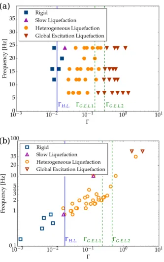
C. Phase diagram controlling liquefaction occurence and type
Three general types of behavior have been identified and analyzed from both a macromechanical and a mi-cromechanical point of view. We will now examine under which conditions these different behaviors occur, derive a phase diagram as function of the control parameters, and check using experiments and simulations the theory derived in subsection I B for the transition between these three behaviors. For this purpose, we make a systematic series of experiments and simulations at various frequen-cies and amplitudes. The frequenfrequen-cies range from 7 Hz to 24 Hz for simulations and from 0.15 Hz to 50 Hz for ex-periments and the acceleration range from 0.01 m s−2 to 1 m s−2 for simulations and from 0.001 m s−2 to 4 m s−2 for experiments. We link each experimental and sim-ulation run to one of the three behaviors, rigid, H.L. or G.E.L., according to the categorization criteria explained in subsections II C 2 and II C 3. On the phase diagram, Fig. 12, we show the results of this systematic study for the numerical simulations (a) and the experiments (b). Γ is represented on the horizontal axis and the frequency of shaking is on the vertical axis. Each simulation and ex-periment is plotted with a particular symbol representing the associated behavior: blue squares for rigid states, or-ange discs for H.L. states and red triangles pointing down for G.E.L. states, according to the thresholds defined in section II C. A particular liquefaction behavior, repre-sented by purple triangles pointing up and called slow liquefaction, will be further discussed in the next section. It is related to a few experiments and simulations which don’t follow the same master curve as all other experi-ments and simulations. As predicted by the theory and confirmed by figure 12 both for simulations and experi-ments, the main control parameter determining whether liquefaction happens, and what type of liquefaction, is the value of the normalized peak ground acceleration Γ. Two possibilities are shown for ΓG.E.L.: ΓG.E.L.2
corresponding to the theoretical sliding threshold of an initialy emerged intruder (Eq. (9) of section I B) and ΓG.E.L.1 corresponding to the sliding threshold
of an intruder which is initially partially immersed. ΓG.E.L.1 is calculated as ΓG.E.L.1 = µ(1 −
VB.im(0)ρw
VBρB ),
with the initial immersed volume VB.im(0) of 50% for
the simulations and 12% for experiments. ΓG.E.L.1 is
smaller than ΓG.E.L.2 because the buoyancy applied
on the intruder immersed volume reduces the acceler-ation needed to make it slide on the particles underneath. Let us examine, from Fig. 12, the deviation between the phase boundaries derived experimentally or numer-ically, and those obtained with the simple analytical model, considering ΓG.E.L.1 the threshold corrected for
bound-FIG. 12. Phase diagram of the numerical simulations (a) and of the experiments (b). Each simulation or experiment is plot-ted according to its reduced acceleration Γ and its frequency. The behaviors are determined following the thresholds de-fined in subsections II C 2 and II C 3. Squares correspond to an observed rigid behavior, circles and triangles pointing up to H.L. behavior, and triangles pointing down to G.E.L. havior. The boundaries theoretically derived in section I B be-tween these three regimes are the vertical lines: Γ = ΓH.L.for
the rigid/H.L. boundary, and Γ = ΓG.E.L.1or Γ = ΓG.E.L.2are
two possibilities for the H.L./G.E.L. boundary. These bound-aries match well with the observed symbol changes, both in experiments and in simulations.
ary between rigid and H.L. state is very well reproduced by both the simulations and the experiments. Concern-ing the boundary between H.L. and G.E.L. the phase diagram of the simulations shows again a very good fit beween theory and experiments. For the experiments, the setup limitations do not allow too many experiments at very large accelerations. A dispersion of the behavior results is observed, with a gradual transition from H.L. to G.E.L.. The transition nonetheless happens at a central value around the one predicted by theory. At first order, the two theoretical boundaries ΓH.L.and ΓG.E.L. capture
very well the location of the different behaviors observed
with numerical simulations and experiments. The sim-ilarity found in the results between simulations, experi-ments and theory are thus satisfactory, and validate the explanation proposed for the physics of liquefaction.
D. Comparison of the final position and the isostatic position
In the previous paragraph we show that the behavior of the intruder above the shaken granular media can be sorted into three cases according to the imposed acceler-ation, as we expected given the theoretical analysis. We will now study what is the final position of the intruder during H.L. and the velocity at which it approaches it. During the H.L. regime, as a first approximation, if the vertical friction forces on the intruder average to zero after penetration, the intruder will approximately ap-proach the theoretical isostatic position dictated by its weight and the buoyancy (section I B 3). The experimen-tal and numerical setup enables to test whether this ap-proximation holds or fails, by measuring precisely the final vertical position of the intruder for a comparison with the isostatic position. For each simulation the ratio of the final position of the intruder to its isostatic po-sition, h(∞)/hISO, is represented on Fig. 13. Different
symbols correspond to different behaviors observed fo the simulations: rigid, slow liquefaction, H.L. or G.E.L.. We
FIG. 13. Final depth of the intruder scaled by its isostatic depth, h(∞)/hISO, as function of the dimensionless imposed
peak ground acceleration Γ. The markers correspond to the behavior of the medium, rigid, slow liquefaction, H.L. or G.E.L.
see that when Γ rises, the ratio rises towards 1, i.e. the intruder approaches its isostatic depth. The ratio is 0.2 for the slow liquefaction case, and between 0.5 and 1 for most H.L. cases. When Γ exceeds 0.2 to 0.3 the media displays G.E.L. behavior, and this ratio lies between 0.7 and 1 for most cases, but decreases below 0 for some cases of intense shaking, which means that instead of sinking,
the intruder rises above the grains. These particular re-sults are a demonstration of the Brazil nuts effect where the intense shaking and the friction between grains result in a vertical force opposed to the weight of the intruder. This graph demonstartes that the isostatic position is a relatively good approximation for the final position dur-ing H.L., although the results are somewhat dispersed, especially at relatively low acceleration.
E. Penetration dynamics in liquefied cases 1. Data collapse and master curve
To understand further the phenomenon of sinking of an object inside a liquefied granular medium, we investigate the dynamics of the intruder, and how it penetrates to-wards its equilibrium position in the liquefactions cases. For simulations made at different amplitudes and fre-quencies but at the same peak ground velocity (PGV), one can observe that all the curves align together, see Fig. 14. This observation guides us to collapse the
im-FIG. 14. Normalized emerged volume χin(t) as function of
time in simulations at different amplitudes and frequencies, but with an approximatively constant PGV of 0.012 m/s. It can be seen that simualtions ran with the same PGV follow the same master curve. The theoretical relaxation of the in-truder for a PGV of 0.012 m/s, calculated in part III F, is plotted in a thick gray curve.
mersed volume vs time curves, and establish a master curve followed by all the simulations. Considering sim-ulations made with any amplitude and frequency, whose sinking vs time curves are shown on Fig. 15 on top, we are able to collapse all curves of evolution of the sink-ing depth by plottsink-ing it as function of a reduced time corresponding to the cumulated strain imposed by the oscillations, i.e. the time multiplied by the PGV: see Fig. 15(b). This shows that the speed of penetration of the intruder mainly depends on the peak velocity of the shaking.
FIG. 15. (a) Normalized emerged volume of the intruder as function of time χin(t) in a set of simulations; (b) Normalized
emerged volume as function of a normalized time, multiplied by the PGV of each respective run, for the same set of sim-ulations. The curves show a reasonable collapse on a master curve. In thick grey we add the theoretical relaxation of the intruder. The calculation is made in part III F.
2. Exponential relaxation and characteristic time
Concerning the shape of the sinking curves, a natu-rally expected shape is an exponentially or a logarithmic decreasing function. Indeed, on one hand linear systems relax towards equilibrium following an exponential evo-lution. On the other hand, in non linear systems close to jamming or pinning, slow relaxation or creep dynamics often lead during long time to a deformation logarith-mic in time. This is for example the case for dry grain packings compacting under vibrations, [61, 62], for creep in fracture propagation [63] or for deforming rocks [64]. We use semi-logarithmic representations to verify if the sinking results reveal one of these behaviors. Fig. 16 dis-plays the sinking of our intruder during one simulation – characteristic of the majority of the simulation cases. Fig. 16 (a) shows an attempt to a logarithm fit to the sinking of the intruder, and Fig. 16 (b) shown an expo-nentially decreasing fit attempt to the same data. For both cases we presented the result first with a semiloga-rithmic scale, where an exponential behavior would corre-spond to a straight line, and then with a linear scale. The exponentially decreasing function fits the vast majority of the liquefied simulations whereas the logarithmically decreasing ones fit only few simulations whose behavior was hard to distinguish between rigid and liquefied - these correspond to the few slow liquefaction cases that will be developed in further detail in Sec. III G. When the
gran-FIG. 16. Descent laws for intruders: fitting the normalized emerged height of the intruder H(t) as function of time. We apply a logarithmic fit to the simulation data (dark blue curve) in (a), (b) and an exponential fit in (c), (d). Fits are shown in light gray. Sinking of the intruder is best modelled by an exponential decrease of the height.
ular medium is well liquefied we can then assume that the intruder follows an exponential sinking toward its equilibrium position. This will be confirmed by a phys-ical explanation later on. We apply the exponential fit to every simulation categorized as liquefied and system-atically compute the half-life times. The procedure is semi-automatic. We compute the intruder normalized emerged height H defined as follows: H(t) = h(∞)−h(t))h(∞)−h(0) with h(t) the immersed height previously introduced and h(∞) the immersed height at isostatic position. H is defined by the same principle as Xin (equation 17), i.e.
as a normalized height which starts at 1 for every case and goes to 0 if the final immersed height of the intruder reaches h(∞), the isostatic position. We plot H with a logarithmic y-axis, as on Fig 16(c), and we pick manually the duration corresponding to a straight line (orange line on the plot). This duration should not be smaller than 3 seconds. We then apply a linear regression to the normal-ized emerged height H, using the selected duration and a logarithmic y-axis, for different values of h(∞): the linear regression is applied to 15 values of h(∞) equally spaced between the isostatic position minus 15% and the
isostatic position plus 15%. We keep the result which gives the largest correlation coefficient. Eventually, from the slope of the linear regression λ, we obtain the half life time as t1/2= ln(2)/λ.
FIG. 17. (a) Half-life time for sinking of intruders in sim-ulations, as a function of the peak ground velocity (PGV). The shapes of the markers correspond to the shaking fre-quency. The thick grey line plots theoretical values for the half-life time according to the calculation made in part III F, i.e. t1/2= 0.02m/PGV. (b) P GV × t1/2, product of the
Half-life time by the PGV, as a function of the PGV. Part III F predicts that this product is a constant.
We are now able to plot the half-life time of the simu-lations according to the PGV of the imposed shaking, see Fig. 17. Different markers are used for different frequen-cies. It is clear from the collapse of Fig. 15 and from the half-life time dependency of Fig. 17 that the half-life time is proportional to the inverse of the PGV as all the points follow the same master curve regardless of the frequency. At first order the master curve is the inverse function. We can now present a physical explanation for the expo-nential sinking and for the half-life times dependence on the PGV.
F. Theoretical point of view
The exponential descent of intruders into granular me-dia has already been reported in a related study by [14]. They used real sand and a steel cylinder as an intruder. To understand the origin of this exponential behavior, we will make an approximate mechanical analysis of the granular medium rheology. There are mainly two forces acting on the intruder, apart from its weight: A buoyancy force coming from the fluid and a frictional force exerted
by the solid contacts with the granular medium. A recent study [27] shows that in dry granular media shaken hori-zontally, the frictional force opposing the intruders sink-ing, acts locally normal to the intruder surface. Following the authors of that study, we assume that this stays valid in the saturated case, and since the penetration speed is low, we assume that the frictional force is proportional to the speed of the intruder in the medium. Newton’s second law applied to the intruder and projected on the vertical axis can be phrased as:
ρBV
d2u
dt2 = −ρBV g + ρeffVim(u)g − α
du
dt, (18) where u is the vertical displacement of the intruder, ρBits
density V its volume, and ρeff the effective density of the
saturated granular medium. We checked that ρBVd
2u
dt2 is
very small relative to the other forces. In this case, the equation of motion can be simplified as:
du dt =
1
α(−ρBV g + ρeffVim(u)g). (19) One solution of equilibrium exists when ρB< ρeff. When
this solution, called ueq, is reached, the term dudt is equal
to 0. Thus
ρeffVim(ueq) = ρBV.
We focus on the dynamics near the equilibrium state, in which case:
Vim(u) = Vim(ueq) +
dVim
du |ueq(u − ueq)
The term dVim
du |ueq is linked to a characteristic surface of
the intruder. It represents the disc of intersection be-tween the intruder at equilibrium position and the effec-tive fluid surface. As the equilibrium position is close to total immersion, the intersection between the intruder and the effective fluid surface decreases when the intruder approaches its equilibrium, and so dVim
du |ueq is a negative
term. Thus we will write β = −dVim
du |ueq, where β is
positive. Eq. (19) becomes: du
dt = 1
α(−ρBV g + ρeff(Vim(ueq) − β(u − ueq))g) . Thanks to the expression of the equilibrium solution Vim(ueq), this becomes:
du dt =
βgρeff
α (ueq− u).
We finally reach a linear differential equation. Using u0=
u(t = 0), the initial position, we obtain the following solution for u:
u(t) = (u0− ueq)e
−βgρeff
α t+ ueq. (20)
So finally, after having assumed a negligible acceleration for the intruder and a frictional force proportional to the
velocity of the intruder, we find that the movement of the intruder around its equilibrium position follows an exponentially decreasing law.
Concerning the half-life time of penetration, our results allow to provide an expression for α. In Eq. (20), we have an expression for the half-life time t1/2:
t1/2=
ln(2)α βgρeff
. (21)
We can measure a particular half-life time with figure 14. The simulations plotted in this figure have a PGV of V0= 0.012 m/s and the half-life time is equal to T0= 1.7
s. We can assume that
t1/2= T0F (A 2πf ) (22)
where F is a function of ( 2πAf ) the PGV of the simula-tions with F (V0) = 1. Then we use the observation made
in figure 15 and 17, namely that for simulations having different PGV, the alignement is obtained by multiplying the time axis by the PGV. The interpretation is that the caracteristic time of the decreasing of Xin, the half-life
time in the case of an exponential decrease, is a function of the form
t1/2=
C
A 2πf (23)
where C is a constant. We can equate the two expres-sions 22 and 23 in order to find C = T0V0= 0.02 m. In
figures 15 and 14, we have drawn the theoretical lines corresponding to an exponential decrease from 1 to 0 with the caracteristic time defined by the half-time t1/2
of this last Eq. (23). The agreement with the halftimes extracted from the simulations demonstrates the consis-tency of this expression. Combining expressions 21 and 23 provides an expression for α, which determines the prefactor of the friction law for the penetration of the intruder in the shaken granular medium, as function of β, the cross section of the intruder close to the isostatic position, the density of the medium and the PGV A2πf :
α = βgρeff ln(2)
T0V0
A 2πf
α may be viewed as an effective viscosity coefficient.
G. Particular case of slow liquefaction following logarithm penetration
The dynamics of the intruder described above predicts the behavior of most of the liquefied (H.L.) simulations and experiments, yet fails to reproduce the behavior in a few cases. Indeed among the simulations classified as liquefaction state, there are some few cases where the sinking of the intruder does not follow the same trend as described above. When the intruder movement is com-pared to other simulations ran at the same PGV, the