Uncertainties in selected surface water quality data

(1)

HAL Id: hal-00298776

https://hal.archives-ouvertes.fr/hal-00298776

Submitted on 21 Sep 2006

HAL is a multi-disciplinary open access

archive for the deposit and dissemination of sci-entific research documents, whether they are pub-lished or not. The documents may come from teaching and research institutions in France or abroad, or from public or private research centers.

L’archive ouverte pluridisciplinaire HAL, est destinée au dépôt et à la diffusion de documents scientifiques de niveau recherche, publiés ou non, émanant des établissements d’enseignement et de recherche français ou étrangers, des laboratoires publics ou privés.

Uncertainties in selected surface water quality data

M. Rode, U. Suhr

To cite this version:

M. Rode, U. Suhr. Uncertainties in selected surface water quality data. Hydrology and Earth System Sciences Discussions, European Geosciences Union, 2006, 3 (5), pp.2991-3021. �hal-00298776�

(2)

HESSD

3, 2991–3021, 2006

Uncertainties in surface water quality

data

M. Rode and U. Suhr

Title Page Abstract Introduction Conclusions References Tables Figures J I J I Back Close

Full Screen / Esc

Printer-friendly Version

Interactive Discussion

EGU Hydrol. Earth Syst. Sci. Discuss., 3, 2991–3021, 2006

www.hydrol-earth-syst-sci-discuss.net/3/2991/2006/ © Author(s) 2006. This work is licensed

under a Creative Commons License.

Hydrology and Earth System Sciences Discussions

Papers published in Hydrology and Earth System Sciences Discussions are under open-access review for the journal Hydrology and Earth System Sciences

Uncertainties in selected surface water

quality data

M. Rode and U. Suhr

UFZ – Centre for Environmental Research, Department of Hydrological Modelling, Brueckstrasse 3a, 39114 Magdeburg, Germany

Received: 24 February 2006 – Accepted: 9 June 2006 – Published: 21 September 2006 Correspondence to: M. Rode (michael.rode@ufz.de)

(3)

HESSD

3, 2991–3021, 2006

data

M. Rode and U. Suhr

Full Screen / Esc

Interactive Discussion Abstract

Monitoring of surface waters is primarily done to detect the status and trends in wa-ter quality and to identify whether observed trends arise form natural or anthropogenic causes. Empirical quality of surface water quality data is rarely certain and knowledge of their uncertainties is essential to assess the reliability of water quality models and 5

their predictions. The objective of this paper is to assess the uncertainties in selected surface water quality data, i.e. suspended sediment, nitrogen fraction, phosphorus frac-tion, heavy metals and biological compounds. The methodology used to structure the uncertainty is based on the empirical quality of data and the sources of uncertainty in data (van Loon et al., 20061). A literature review was carried out including additional 10

experimental data of the Elbe river. All data of compounds associated with suspended particulate matter have considerable higher sampling uncertainties than soluble con-centrations. This is due to high variability’s within the cross section of a given river. This variability is positively correlated with total suspended particulate matter concen-trations. Sampling location has also considerable effect on the representativeness of 15

a water sample. These sampling uncertainties are highly site specific. The estimation of uncertainty in sampling can only be achieved by taking at least a proportion of sam-ples in duplicates. Compared to sampling uncertainties measurement and analytical uncertainties are much lower. Instrument quality can be stated well suited for field and laboratory situations for all considered constituents. Analytical errors can contribute 20

considerable to the overall uncertainty of surface water quality data. Temporal autocor-relation of surface water quality data is present but literature on general behaviour of water quality compounds is rare. For meso scale river catchments reasonable yearly dissolved load calculations can be achieved using biweekly sample frequencies. For suspended sediments none of the methods investigated produced very reliable load 25

1

van Loon, E., Brown, J., and Heuvelink, G.: A framework to describe hydrological uncer-tainties, Part of this Special Issue “Uncertainties in hydrological observations”, Hydrol. Earth Syst. Sci. Discuss., in preparation, 2006.

(4)

HESSD

3, 2991–3021, 2006

data

M. Rode and U. Suhr

Full Screen / Esc

EGU estimates when weekly concentrations data were used. Uncertainties associated with

loads estimates based on infrequent samples will decrease with increasing size of rivers.

1 Introduction

The objective of this paper is to give an overview of the uncertainties one faces in 5

dealing with selected surface water quality data. Monitoring of surface waters is pri-marily done to detect the status and trends in water quality and to identify whether observed trends arise form natural or anthropogenic causes. Most important environ-mental problems of surface water quality are eutrophication, acidification and emission dispersion where non point source pollution became increasingly importance within 10

the last decades. Eutrophication of inland and coastal waters is a world-wide environ-mental problem and serious efforts are needed to reduce emissions and improve the situation (e.g., Ryding and Rast, 1989). The effect of eutrophication is high production of plankton algae (“algal blooms”), excessive growth of weeds and macroalgae, lead-ing to oxygen deficiency, which in turn leads to fish kills, reduced biological diversity, 15

bottom death and toxic substances in the water. The problems related to acidifica-tion are mainly found in the northern hemisphere, and is caused by air-born pollutants that causes acid conditions when deposed on sensible soils. Regarding dispersions of water-related pollutants, it may be important to assess accidental emissions or indirect side-effects. Regarding the marine environment reductions of nutrient and contaminant 20

loads are primary objectives.

Beside the identification of the status and trends surface water quality data are es-sential for the application of stochastic and deterministic water quality models (Trudgill, 1995; Arheimer and Olsson, 2003). Water quality models are generally used to sepa-rate the contributions from various sources and to distinguish between natural variabil-25

ity and anthropogenic impact. Predictive models are commonly used for integrating and testing of alternative management strategies. This enables an efficient environmental

(5)

HESSD

3, 2991–3021, 2006

data

M. Rode and U. Suhr

Full Screen / Esc

Interactive Discussion control and the development of management practices. Water quality modelling allows

also the prediction of future scenarios.

Clearly, pollution and acidification are the most important reasons for past and cur-rent water quality model development. The pollution context includes models of the transport of nutrients, organic material, oxygen balance, heavy metals and organic 5

compounds through soil profiles, hillslopes and catchment scale as well as the mod-elling of downstream changes in pollutant loading (James, 1993). Closely related to the pollution context is the simulation of soil erosion and sediment transport on the catchment scale. The group of river water quality models simulate the substance transformation in river channels in a mechanistic way and transport calculations are 10

based on hydraulics. These models are able to simulate biological variables due to pri-mary production and the transport of pollutants like heavy metals and organic chemical (exposure models). The acidification context includes short and long-term catchment scale models of chemical reactions. Most important variables are the ph-value and re-lated heavy metals as well as the Si-fraction. Knowledge of the uncertainties in surface 15

water quality data is essential to assess the reliability of water quality models and their predictions like e.g. scenario analyses.

1.1 Selected groups of variables

Monitored surface water quality variables are numerous. This is especially true for the group of organic chemicals, e.g. the Water Framework Directive defined 33 prior-20

ity constituents and constituents groups. Therefore a selection of the most important water quality variables has to be made with special regard to modelling aspects. We selected the surface water quality constituents listed in Table 1 according to their im-portance, their behaviour and the model needs. Recent evidence indicates that the majority of fluvial trace element and some major ion transport occur in association with 25

suspended sediments (Horrowitz 1995, 1997). This is also true for organic chemicals with high adsorption coefficients. Furthermore, suspended sediments are important for total phosphorus transport in surface waters. Suspended sediments concentrations

(6)

HESSD

3, 2991–3021, 2006

data

M. Rode and U. Suhr

Full Screen / Esc

EGU have extremely high spatial and temporal variability and are therefore associated with

high sampling uncertainties. Nutrients like phosphorus, nitrogen and silicon are limiting constituents for primary production especially in large rivers and the marine environ-ment. Primary production influences the oxygen concentrations and impacts also the pH-value. Additionally, some inorganic nitrogen compounds have acute chronic effects 5

on aquatic organisms and are relevant for drinking water supply. Biological variables like BOD are the most important indicators for waste water emissions and highly af-fect oxygen concentrations. Chl a, which is commonly used as an indicator for algal biomass, is also relevant for drinking water supply from surface waters (bank filtration). Biological variables are highly variable in space and time and are associated with high 10

sampling and analytical uncertainties.

The objective of this paper is to assess the uncertainties in selected surface water quality data, i.e. suspended sediment, nitrogen fraction, phosphorus fraction, heavy metals and biological compounds. The considered variables in this chapter are listed in Table 1. For each variable the most commonly used analytical method was selected. 15

They can be grouped in sediments, nutrients (mainly nitrogen and phosphorus com-pounds), biological variables, selected major ions and trace elements (see Sect. 2). Due to the importance of the calculation of river load and the large uncertainties as-sociated with different calculation procedures one section on this topic is added. All constituent sections consider several information on uncertainty category, empirical 20

uncertainty, quality of methods, the longevity of the uncertainty information and the times and locations for which the uncertainty information is valid.

1.2 Importance of different uncertainty factors

The most important uncertainty factors of surface water quality data are sampling and measurement or analytical uncertainties. Conceptual problems and conversion of data 25

transfer are of minor importance. Sampling uncertainties can be distinguished between uncertainties related to the selection of a representative sampling location, represen-tative samples at a given river cross section and the choice of an appropriate sample

(7)

HESSD

3, 2991–3021, 2006

data

M. Rode and U. Suhr

Full Screen / Esc

Interactive Discussion frequency e.g. for calculation of representative loads at a given location (see Table 2).

The choice of a sampling location may have considerable impact on the measured concentration of a given variable. In streams and small rivers with high flow velocities water quality compounds are in general well mixed within the cross section due to high turbulence of the flow. Temporal and spatial variations of water quality variable concen-5

trations in a given river reach are determined by point sources and the transformation rate of the specific water quality variable. In large rivers the selection of a represen-tative sampling location is much more difficult due to much longer time spans of total mixing of larger tributaries. An example is given for the Chl a concentrations in the Elbe river in Fig. 1. In the case of low flow conditions total mixing of the Saale tributary 10

within the Elbe river needs about 70 km.

The Saale river is the largest German tributary of the Elbe river. Within this river reach considerable differences for most water quality variables can be observed on the right and left bank of the river (see also Guhr et al., 2000). The choice of a represen-tative sampling within a cross section depends on the variability of a given compound, 15

where the variability of suspended particulate matter and associated compounds in general is much larger than of soluble compounds. This variability is highly specific for each river system and river location. Therefore it is not possible to give general quantitative estimates on the uncertainties associated with sampling in a given cross section. It should be apparent that the collection of a single “grap” sample at a single 20

depth, from the centroid of flow or from the bank is unlikely to produce representa-tive samples especially of suspended particulate matter and associated constituents. Some qualitative explanations are given in the following chapters for the different water quality groups. The same is true for the choice of representative sampling frequencies for reliable load calculations.

25

The methodology used to structure the uncertainty is based on a fourfold distinction between the empirical quality of data, the sources of uncertainty in data, the fitness for use of data and the goodness of an uncertainty model (van Loon et al., 20061). In this paper we focus on the empirical quality of data and its sources of uncertainty through

(8)

HESSD

3, 2991–3021, 2006

data

M. Rode and U. Suhr

Full Screen / Esc

EGU a literature review and additional experimental data of the Elbe river. Most water

qual-ity variables can be grouped in similar uncertainty categories (e.g. B1 or D1). Also the analytical uncertainties can be stated for nearly all variables as M1 and instrument quality is always well suited for the field situation and calibrated if standard procedures are used (see Table 3). The overall method is always approved standard in well estab-5

lished disciplines. For all variables the uncertainty information is known to change over time. Information on autocorrelation of time series data is rare in the literature. If pos-sible additional information is given in the following sections. Quantitative estimates on uncertainties for the variable groups like coefficients of variation (CV) of pdf (see Table 5) are restricted to measurement and analytical uncertainties due to the lack of 10

information and site specific characteristics of other uncertainty information. The given values on mean standard deviations are general estimates for the analytical methods considered in Table 1. The estimation of uncertainty in sampling can only be done by taking at least a proportion of samples in duplicates. A detailed review of techniques for quantification and comparison of sampling and analytical sources of uncertainties 15

is given e.g. by Ramsey (1998).

2 Groups of variables

2.1 Suspended sediments

Suspended sediments are defined as the portion of total solids retained by a filter. The currently accepted operational definition of the filter size is a 0.45 µm membrane 20

filter (Horowitz, 1997). Suspended sediments are a major carrier of a varity of min-eral and organic constituents. Obtaining representative samples of suspended sedi-ments is, therefore, of fundamental importance in studies concerned with quantifying geochemical fluxes and understanding water quality in fluvial systems. Even in wa-ter with suspended sediment concentrations <10 mg/l, these solids are responsible for 25

(9)

HESSD

3, 2991–3021, 2006

data

M. Rode and U. Suhr

Full Screen / Esc

Interactive Discussion representative samples of suspended sediments is of paramount importance, as it is

impossible to sample and analyse an entire water body.

The uncertainty category of suspended sediments can be defined as D1, since au-tomatic samplers are able to collect samples with high temporal resolution, e.g. 5 min intervals. In many cases suspended sediments are also sampled on regular daily, 5

weekly or biweekly intervals. Empirical uncertainties encountered with suspended iments can be defined as type M1 (probability distribution). In general, suspended sed-iment concentrations have extremely high variations within the cross sectional area of a given river. When both sand-sized (>63 µm) and silt/clay-sized (<63 µm) particles are present in a stream, the concentrations of suspended sediments tend to increase 10

with increasing distance from the river bank. This is a common pattern and results from an increase in stream velocity (discharge) due to decreasing frictional resistance from the river banks and the river bed (Vanoni, 1977). Vertical concentrations of fluvial suspended sediments tend to increase with increasing depth. This is also due to the increase of sand sized material. This occurs because the velocity (discharge) in most 15

rivers, under normal flow conditions, is insufficient to distribute coarse material homo-geneously. Hence the majority of sand sized particles tend to be transported near the river bed. Therefore it should be apparent that collection of a grab sample at a single depth, from the centroid of flow or from one bank is unlikely to produce representative samples of suspended sediments (Horowitz, 1997; Horowitz et al. 1989).

20

Representative suspended sediment sampling requires a composite of a series of depth- and width-integrated isokinetic samples obtained either at equal discharge or at equal width increments across a river (Horowitz et al., 1990; Horowitz, 1997). The increased velocities and turbulence found in the centre of many rivers leads to lateral variation of suspended sediment concentrations with elevated values in the middle of 25

the cross section. Most of this variation in suspended sediment concentration in a sec-tion is accounted for by the sand fracsec-tion (>63 µm), hence the variasec-tions in the case of sediment concentrations dominated by silt and clay fraction, e.g. under low flow con-ditions, is less important. Investigations into vertical variations in sediment

(10)

concentra-HESSD

3, 2991–3021, 2006

data

M. Rode and U. Suhr

Full Screen / Esc

EGU tions conducted by Wass and Leeks (1999) revealed well mixed conditions for English

rivers. These rivers varied in catchment size between 484 and 8231 km2 and mean suspended sediment concentrations less than 60 mg l−1 and maximum suspended sediment concentrations less then 1600 mg l−1. The errors of single samples within a cross section compared with measurements made using depth-integrated samplers 5

across a section leaded to errors ranging from 2 to 12% (Wass and Leeks, 1999). It is well known, that suspended sediment concentrations also have high tempo-ral variations. Although a number of factors other than just discharge are involved (e.g. grain-size distribution, shear stress, turbulence, stream-bed gradient), there is a widely held belief that in fluvial systems, as discharge increases, suspended concen-10

trations also increases (Horowitz, 1997). Commonly about 90% of the annual load is transported within only about 10% of the time (e.g. Walling et al., 1992; Horowitz, 1995). Sampling frequency for flux estimates becomes dependent on the time period of concern (daily, weekly, monthly, yearly) and the amount of acceptable error associated with these estimates.

15

Sample volume should be chosen to yield between 2.5 and 200 mg dried residue. Commonly samples are dried by 103 to 105◦C in an oven, cool in a desiccator to balance the temperature, and weight. The standard deviation was 5.2 mg/L (coe ffi-cient of variation 33%) at 15 mg/L, 24 mg/L (10%) at 242 mg/L, and 13 mg/L (0.76%) at 1707 mg/L in studies by two analysts of four sets of 10 determinations each. Single-20

laboratory duplicates analyses of 50 samples of water and wastewater made with a standard deviation of differences of 2.8 mg/L. (Standard Methods, 1998). This indicates that the absolute analytical measurement error is nearly constant and the percentage measurement error decreases with increasing suspend sediment concentrations. For suspended sediment concentrations problems related to collecting representative sam-25

ples (one that encompass the range of spatial and temporal variability at a site) are of primary concern compared to analytic uncertainties.

(11)

HESSD

3, 2991–3021, 2006

data

M. Rode and U. Suhr

Full Screen / Esc

Interactive Discussion 2.2 N-Fraction

In surface waters the forms of nitrogen of greatest interest are, in order of decreas-ing oxidation state, nitrate, nitrite, ammonia and organic nitrogen. All these forms of nitrogen are biochemically interconvertible and are components of the nitrogen cycle. Regarding nitrate the automated cadmium reduction method (NO₃-CRM) is a com-5

monly used method for nitrate analytical determination. Nitrate can be determined over a range of 0.5 to 10 mg N/l. Sample turbidity may interfere the analytical proce-dure. Table 4 shows the impact of laboratory induced uncertainties on nitrate data. Three laboratories used the same automated systems but having slightly different con-figurations.

10

In a single laboratory using surface water samples at concentrations of 100, 200, 800, and 2100 µgN/L, the standard deviations were 0, ±40, ±50, and ±50 µgN/L, re-spectively. These findings for nitrate on decreasing relative bias with increasing con-centrations are typical also for other water quality constituents and most analytical methods. Precision and bias for the system described are believed to be comparable 15

(Standard Methods, 1998). The standard deviations reported from the Laboratory of the UFZ Environmental Research Centre in Magdeburg are with a maximum of 3.3% similar to these findings. The analytical limit is about 50 µgN/L. The NO₃-Electrode Method (EM) has detection limits between 0.14 and 1400 mg NO₃-N/L and pH-values have to be held constant. Over the range of the method, precision of ±0.4 mV, corre-20

sponding to 2.5% in concentration, is expected (Standard Methods, 1998). Nitrite is an intermediate oxidation state of nitrogen, both in the oxidation of ammonia to nitrate and in the reduction of nitrate. Mean standard deviations change slightly depending on the analytical method. Colorimetric methods may have somewhat higher bias than the Ion Chromatography (IC) method. In general measurement errors should be not higher 25

than 6%. The bias will decrease with increasing concentrations.

Ammonia is present naturally in surface and wastewaters. Its concentration is gener-ally low in groundwater because it adsorbs to soil particles and clays and is not leached

(12)

HESSD

3, 2991–3021, 2006

data

M. Rode and U. Suhr

Full Screen / Esc

EGU from the soils. Ammonia concentration can vary between 10 µg/l ammonia nitrogen in

some natural groundwater systems and 30 mg/L in some wastewater. Ammonia con-centrations in surface water, e.g. due to wastewater inputs, tend to decrease rapidly by nitrification. Mean standard deviation of analytical methods have values between 5 and 8% where the IC method showed highest standard deviation of up to 11% (DEV, 2000). 5

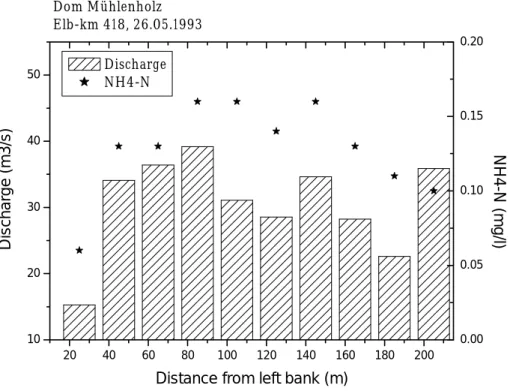
The lowest bias is associated with the flow injection analysis (Standard methods 1998). In general, soluble compounds like ammonia have much lower concentration variation within a cross section of a given stream or river compared to suspended sediment as-sociated compounds. Nevertheless during low flow season and high biological activity also soluble concentrations of reactive compounds may vary considerably. Figure 2 10

shows deviations of ammonia concentrations within the cross-section of the Elbe River of more than 50% of the mean value. This is due to high algal biomass concentration and associated nutrient uptake or higher nitrification rates in the proximity of the banks, which are modified by groynes. These effects may be much more important for larger rivers than for small rivers and streams due to their higher turbulence and mixing within 15

the cross section.

Studies on autocorrelation in nitrogen time series mainly focus on trend analysis and the determination of seasonal trend components (Lehmann and Rode, 2001; Worral and Burt, 1999). Published studies on simple temporal autocorrelation of nitrogen time series are rare and are restricted on weekly nitrate data. No studies were found on the 20

systematic analyses of temporal autocorrelation functions on time series data. Markus et al. (2003) showed high autocorrelation of lag-one nitrate-N for the Sangamon River in the Midwestern United States. Two week temporal autocorrelation was lower but still higher than 0.6. During high nitrate concentrations seasonal autocorrelations seemed to be higher than during low concentrations (Markus et al., 2003). Correlation between 25

nitrogen compounds and other water quality constituents are frequent and depend on site specific nitrogen loadings e.g. the share of point and non point sources pollution. In general the correlation between discharge and nitrate is week due to the strongly non linear relationship between discharge and nitrate concentration.

(13)

HESSD

3, 2991–3021, 2006

data

M. Rode and U. Suhr

Full Screen / Esc

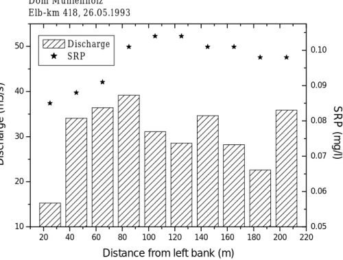
Interactive Discussion 2.3 P Fraction

Phosphorus occurs in natural waters and in wastewaters almost solely as phosphates. They occur in solution, in particles or detritus, or in the bodies of aquatic organisms. Phosphorus is essential to the growth of organisms and can be the nutrient that lim-its the primary productivity of a water body. Phosphorus analyses embody two general 5

procedural steps: (a) conversion of the phosphorus form of interest like soluble reactive phosphorus, dissolved phosphorus or total phosphorus to dissolved orthophosphate, and b) determination of dissolved orthophosphate by ion chromatography (IC) or col-orimetry. In Table 5 standard deviations of the IC method and additional uncertainty information are given for soluble reactive phosphorus (SRP).

10

The values for the colorimetric determinations are comparable. In determination of total dissolved or total suspended reactive phosphorus, anomalous results may be obtained on samples containing large amounts of suspended sediments. Very often results depend largely on the degree of agitation and mixing to which samples are sub-jected during analysis because of a time-dependent desorption of orthophosphate from 15

the suspended particles (Standard Methods, 1998). Due to strong binding of phospho-rus to suspended particulate matter concentrations of P-compounds vary within the cross sectional area depending on the amount of suspended sediments or organic matter (e.g. algal biomass) in the water body.

Furthermore, dissolved concentrations of P-compounds may vary within the cross 20

section due to differing algal P-uptake (see Fig. 3). In rivers with low algal biomass concentrations or well mixed water bodies the cross sectional variation may not be very important. Suspended sediment concentrations (see above) as well as biological activities vary strongly in space and time. Therefore, autocorrelation of P concen-trations may be much lower than for variables which are less impacted by biological 25

(14)

HESSD

3, 2991–3021, 2006

data

M. Rode and U. Suhr

Full Screen / Esc

EGU 2.4 Heavy metals

Suspended sediment associated heavy metals can display marked short- and long term spatial and temporal variability. Transport of heavy metals occurs mainly in asso-ciation with suspended sediments. Even in waters with suspended sediment concen-trations <10 mg/l, these solids can represent the major carrier for many trace elements 5

(Horowitz, 1997). Therefore, the behaviour of trace elements is very similar to the be-haviour of suspended sediments. Although concentrations of suspended associated compounds can vary strongly within the cross sectional area during high flow and sed-iment concentration conditions (Horowitz, 1997), this variation decrease rapidly during low flow conditions with associated low suspended sediment concentrations. For the 10

Elbe River Cd concentration did not vary systematically within the cross section with high concentrations in the centre of the cross section and low concentrations near the banks (see Fig. 4). These findings are restricted to low suspended sediment con-centrations since in all 14 cross section measurement surveys in 1993 and 1994 in the Elbe River these concentrations were always less than 40 mg/l. As discharge increases 15

it is commonly assumed that the grain size composition of suspended sediments will show a decrease in the clay fraction and an increase in the sand fraction, because of the increase in turbulence and transport capacity for coarser particles associated with higher flows (Horowitz, 1997). Due to the association of heavy metals with more chemically active fine fraction this will in general lead to a decrease of relative sediment 20

associated trace element concentration with increase discharge (Walling et al., 1992). However, it should not be assumed that all rivers will demonstrate this typical grain size behaviour. Walling et al. (1992) showed that rivers often have their very specific transport characteristics and pattern of variation of the concentration of sediment as-sociated substances. In assessing the uncertainties of heavy metal concentration data 25

this leads to the general statement that most monitoring programs lack the necessary resources to sample with sufficient frequency to encompass the degree of temporal variability typical in most fluvial systems. Hence sampling uncertainty, especially for

(15)

HESSD

3, 2991–3021, 2006

data

M. Rode and U. Suhr

Full Screen / Esc

Interactive Discussion sediment related compounds, is much more important than measurement uncertainty,

where high precise and unbiased analytical results are achievable with ICP-based in-strumentations. These measurement uncertainties are presented in Table 5. It is ques-tionable weather this analytical effort is justified when analyzing only a limited number of suspended sediment samples.

5

2.5 Biological fractions

The biological fraction comprises compounds that are mainly impacted by the amount of, the generation or the degradation of organic matter in surface water. Organic matter origin from allochtone (e.g. waste water) or autochtone sources (primary production). The biochemical oxygen demand (BOD) is a measure for the molecular oxygen utilized 10

during a specific incubation period for the biochemical degradation of organic material and the oxygen used to oxidize inorganic material such as sulfides and ferrous iron. Chemical oxygen demand (COD) is defined as the amount of a specific oxidant that reacts with the sample under controlled conditions. COD is often closely related to BOD. Uncertainties associated with different measurement methods for BOD and COD 15

seemed to be comparable and are given in Table 5. They are slightly higher than analytical uncertainties of most nutrients. Analytical uncertainties will decrease with increasing concentrations of DOC and BOD. For further literature see e.g. Standard Methods (1998).

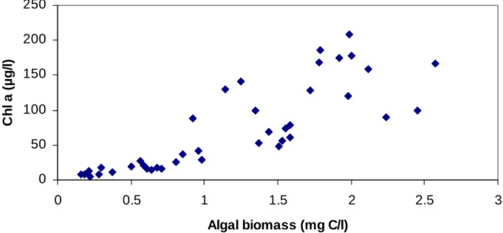
The concentration of photosynthetic pigments like Chlorophyll a is used extensively 20

to estimate phytoplankton biomass where the High-Performed Liquid Chromatogra-phy (HPLC) method is the most commonly used method. Uncertainties of the HPLC method varies between the different pigment types and can vary between 0.5 and 23% with an average value of 10% for seven investigated pigment types (Standard Methods, 1998). Uncertainties compared with other methods like spectrometric or fluorometric 25

methods are similar. These uncertainties are restricted to the quantification of pig-ments and do not reflect the uncertainties associated with these indirect methods to determine phytoplankton biomass. Compared to direct measurement of

(16)

phytoplank-HESSD

3, 2991–3021, 2006

data

M. Rode and U. Suhr

Full Screen / Esc

EGU ton the indirect measurement with pigment concentration is associated with additional

uncertainties since the relationship between both variables is not constant. This rela-tionship strongly depends on the composition of different algal groups and on the cell size of the algae (Creitz and Richards, 1955). Figure 5 shows an example relationship between Chl a and algal biomass. The correlation between biovolume and extracted 5

chlorophyll is not always reliable and this has been widely discussed (Desortova, 1981; V ¨or ¨os and Padisak, 1991). Therefore pigment concentration is a rough estimator of to-tal algal biomass. In large rivers algal concentrations may differ within the river cross section with slightly higher concentrations near the river banks compared to the centre of the river. This is due to larger flow depth in the centre of the cross section. Assuming 10

total mixing of the water column and high algal concentrations the penetration of light is limited.

Regarding the predictability of algal concentrations Hakanson et al. (2003) discussed fundamental principles regulating predictive power of river models for phytoplankton. Their general idea is that the variation of phytoplankton concentrations expressed as 15

CV values determine their overall uncertainty and hence their predictability. They anal-ysed extensive data of different phytoplankton groups on a site in the Danube river and in 19 rivers in the UK. The CV-value for within site variability is always related to very complex climatological, biological, chemical and physical conditions. In the Danube river case study CV values were similar for the different phytoplankton groups but there 20

was a temporal variation in monthly CVs based on data from several years with highest CV during September and October. The mean CV for Chl a based on all data from the River Danube is 0.96, which is close to the median value from 19 river sites in the UK. It has been shown that it is often possible to define characteristic CV-value for a given variable, e.g. chl a values in lakes. It was shown that the CV can give information on 25

(17)

HESSD

3, 2991–3021, 2006

data

M. Rode and U. Suhr

Full Screen / Esc

Interactive Discussion 3 River load calculations and uncertainties

One of the greatest problems associated with the provision of reliable river load data is the assumption that the infrequent samples typically associated with routine water qual-ity monitoring programmes can be used to generate reliable estimates of river loads. In most situations, the accurate assessment of river loads will require a sampling pro-5

gramme specifically designed for this purpose. In considering further the problems of obtaining accurate estimates of river loads, it is useful to make a distinction between the dissolved and the particulate components of river load (Walling et al., 1992). In many situations, the concentrations of most dissolved substances in river water will vary over a limited range and the use of infrequent samples may introduce only relatively limited 10

errors into load assessments, if accurate information on water discharge is available. In the case of particulate- or sediment associated compounds, however, concentrations may vary over several orders of magnitude, particularly during flood events.

Over the last two decades a wide variety of estimation approaches have been devel-oped and used for the estimation of loads of various water quality constituents. These 15

approaches can be divided into averaging, ratio and regression estimators. A short overview is given by Preston et al. (1989) and Cohn (1995). Whereas the two former estimators were used for all water constituents, regression methods have tradition-ally been applied for estimating tributary loads of suspended solids and other related constituents. Guo et al. (2002) demonstrated that in the case of nitrate, which is repre-20

sentative for dissolved compounds, all methods produced relatively small errors (up to 5%) for yearly load calculations in a case study of the Sagamon river in Illinois, USA. The catchment sizes were up to 2375 km2 with nitrate concentrations of up to 10 mg/l nitrate-N. These results were achieved on the basis of weekly and monthly sampling frequencies. In all cases simple averaging and ratio estimators yielded better results 25

than the rating curve method. These results can be supported by the findings of Lit-tlewood (1995) who used averaging estimators for nitrate-N load calculation using the 578 km2British Stour at Langham catchment as a case study. Deviations between

(18)

cal-HESSD

3, 2991–3021, 2006

data

M. Rode and U. Suhr

Full Screen / Esc

EGU culated loads on the basis of a 20 day sampling interval and the actual load were about

5%. In general in river catchments of comparable size biweekly sample frequencies, which are most common for European monitoring programs will lead to reasonable yearly dissolved load calculations.

For suspended sediment flux calculations generally log-log regressions are applied 5

because flow and concentration are assumed to follow a bivariate lognormal distri-bution. Ferguson (1986) and Koch and Smillie (1986) demonstrated that the log-log regression procedure is theoretically biased because of the retransformation from the log scale to the linear scale. Therefore, sediment rating curves can substantially under-predict actual concentrations and loads (see also Asselmann, 2000) and various cor-10

rection factors have been developed to compensate this difficulty (e.g. Ferguson,1986; Walling and Webb, 1988; Asselmann 2000). Using the rating curve technique Horowitz (2003) investigated the impact of sampling frequency on the annual flux estimates for large rivers. For the investigated Mississippi River and Rhine River even collecting a sample as infrequently as once a mouth produced differences only of the order of 15

less than ±20%, regardless of the flux levels compared to true load calculations based on daily samples. Compared to large rivers the uncertainties associated with loads estimates based on infrequent samples will increase for small basins.

An assessment of the likely reliability of suspended sediment loads estimated on the basis of infrequent samples using 1500 km2 basin of the River Exe indicated that 20

errors of the order of ±75% or even greater could arise (see also Walling and Webb, 1981). Errors associated with variability of the concentrations of sediment associated substances are likely to be less (Walling et al., 1992). A comparative study on load estimations methodologies using the River Wharfe at Tadcaster form Webb et al. (1997) showed that simple rating relationships produced estimates of suspended sediment 25

load with the highest level of accuracy, but loads calculated by this procedure still varied from −57% to+29% of the true value using weekly sampling interval. None of the methods investigated produced very reliable load estimates when weekly suspended sediment concentrations data were used.

(19)

HESSD

3, 2991–3021, 2006

data

M. Rode and U. Suhr

Full Screen / Esc

4 Conclusions

This chapter on uncertainties of surface water quality data deals with five different groups of variables listed in Table 1, i.e. suspended sediments, nitrogen fraction, phos-phorus fraction, heavy metals and biological compounds. All data of compounds asso-ciated with suspended particulate matter have considerable higher sampling uncertain-5

ties than soluble concentrations. This is due to high variability’s within the cross section of given river reach. This variability is positively correlated with total suspended par-ticulate matter concentrations. Sampling location has also considerable effect on the representativeness of a water sample. This is especially true for larger rivers with large tributaries and low flow velocities. High sampling effort is needed to get representa-10

tive samples of a given cross section. These sampling uncertainties are highly site specific. The estimation of uncertainty in sampling can only be achieved by taking at least a proportion of samples in duplicates. A detailed review of techniques for quan-tification and comparison of sampling and analytical sources of uncertainties is given e.g. by Ramsey (1998). Compared to sampling uncertainties measurement and ana-15

lytical uncertainties are much lower. Instrument quality can be stated well suited for field and laboratory situations for all considered constituents and most variables can be analysed by direct measurements. All analytical methods have approved standards in well established disciplines. Nevertheless analytical errors can contribute consider-able to the overall uncertainty of surface water quality data. In most cases variation of 20

analytical errors regarding different well approved analytical methods are small. Tem-poral autocorrelation of surface water quality data is present but literature on general behaviour of water quality compounds is rare.

Acknowledgements. The present work was carried out within the Project “Harmonised

Tech-niques and Representative River Basin Data for Assessment and Use of Uncertainty Informa-25

tion in Integrated Water Management (HarmoniRiB)”, which is partly funded by the EC Energy, Environment and Sustainable Development programme (Contract EVK1-CT2002-00109).

(20)

HESSD

3, 2991–3021, 2006

data

M. Rode and U. Suhr

Full Screen / Esc

EGU

References

Arheimer, B. and Olsson, J.: Integration and coupling of hydrological models with water qual-ity models, Applications in Europe, Report of the Swedish Meteorological and Hydrological Institute, Norrk ¨oping Sweden, p. 49, 2003.

Asselmann, N. E. M.: Fitting and interpretation of sediment rating curve, J. Hydrol., 234, 228– 5

248, 2000.

Creitz G. I. and Richards, F. A.: The estimation and characterisation of phytoplankton popula-tion by pigment analysis, J. Mar. Res. 14, 211, 1955.

Cohn, T. A.: Recent advances in statistical methods for the estimation of sediment and nutrient transport in rivers, Rev. Geophys., 1117–1123, 1955.

10

Deutsches Einheitsverfahren (DEV): Selected methods of water analysis, 9th Delivery, Wiley-VCH, Verlag GmbH and Co. KGaA, Weinheim, 1981.

Deutsches Einheitsverfahren (DEV): Selected methods of water analysis, 38th Delivery, Wiley-15

VCH, Verlag GmbH and Co. KGaA, Weinheim, 1997.

20

Desertova, B.: Relationship between chlorophyll-a concentration and phytoplankton biomass in several reservoirs in Czechoslovakia, Int. Revue ges. Hydrobiol., 66(2), 153–169, 1981. Ferguson, R. I.: River loads underestimation by rating curves, Water Resour. Res., 22(1), 74–

76, 1986.

Guo, Y., Markus, M., and Demissie, M.: Uncertainty of nitrate-n load computations for agricul-25

tural watersheds, Water Resour. Res., 38(10), 1185–1197, 2002.

Guhr, H., Karrasch, B., and Spott, D.: Shifts in the processes of oxygen and nutrient balances in the river Elbe since the transformation of the economic structure, Acta hydrochim. hydrobiol, 28(3), 1–7, 2000.

Hakanson, L.: On the principles and factors determining the predictive success of ecosystem 30

models, with a focus on lake eutrophication models, Ecological Modelling, 121, 139–160, 1999.

(21)

HESSD

3, 2991–3021, 2006

data

M. Rode and U. Suhr

Full Screen / Esc

Hakanson, L., Malmaeus, J. M., Bodemer, U., and Gerhardt, V.: Coefficients of variation for chlorophyll, green algae, diatoms, cryptophytes and blue-greens in rivers as a basis for pre-dictive modelling and aquatic management, Ecological Modelling, 169, 179–196, 2003. Horowitz, A. J.: The use of suspended sediment and associated trace elements in water quality

studies, IAHS Special Publication No. 4. IAHS Press, Wallingford, UK, 58 pp., 1995. 5

Horowitz, A. J.: Some thoughts on problems associated with various sampling media used for environmental monitoring, Analyst, 122, 1193–1200, 1997.

Horowitz, A. J.: An evaluation of sediment rating curves for estimating suspended sediment concentrations for subsequent flux calculations, Hydrological Processes, 17, 3387–3409, 2003.

10

Horowitz, A. J., Elrick, K. A., and Hooper, R. P.: The prediction of aquatic sediment-associated trace element concentrations using selected geochemical factors, Hydrol. Processes, 3, 347–364, 1989.

Horowitz, A. J., Rinella, F. A., Lamothe, P., Miller, T. L., Edwards, T. K., Roche, R. L., and Rickert, D. A.: Variation in suspended sediment and associated trace element concentrations 15

in selected riverine cross sections, Environ. Sci. Technol. 24, 1313–1320, 1990. James, A. (Ed.): An introduction to water quality modelling, John Wiley, Chichester, 1993. Koch, R. W. and Smillie, G. M.: Bias in hydrologic prediction using log-transformed regression

models, Water Resour. Bull., 22(5), 717–723, 1986.

Lehmann, A. and Rode, M.: Long-term behaviour and cross-correlations analysis of water 20

quality parameters of the Elbe river at Magdeburg, Germany, Water Res. 35, 2153–2160, 2001.

Littlewood, I. G.: Hydrological regimes, sampling strategies, and assessment of errors in mass load estimates for United Kingdom rivers, Environ. Int., 21(2), 211–220, 1995.

Markus, M., Tsai, C. W.-S., and Demissie, M.: Uncertainty of weekly nitrate-nitrogen forecasts 25

using artificial neural networks, J. Environ. Eng., 129(3), 267–274, 2003.

Preston, S., Bierman, V. J., and Sillimann, S. E.: An evaluation of methods for the estimation of tributary mass loads, Water Resour. Res., 25(6), 1379–1389, 1989.

Ramsey, M. H.: Sampling as a source of measurement uncertainty: techniques for quantifica-tion and comparison with analytical sources, J. Anal. At. Spectrom., 13, 97–104, 1998. 30

Ryding, S. O. and Rast, W. (Eds.): The control of eutrophication of lakes and reservoirs, Man and the Biosphere Series Vol 1, UNESCO and the Parathenon Publishing Group, 1989. Standard methods for the examination of water and wastewater, American Public Health

(22)

Asso-HESSD

3, 2991–3021, 2006

data

M. Rode and U. Suhr

Full Screen / Esc

EGU ciation, American Water Works association and Water Environment Federation (Eds.), 20th

Edition, 1998.

Trudgill, S. T. (Ed.): Solute modelling in catchment systems, John Wiley, Chichester, 1995. Vanoni, V. A.: Sedimentation engineering, American society of Civil Engineers, Manuals and

Reports on Engineering practice No. 54, American Society of Civil Engineers, New York, 5

154–190 and 317–349, 1977.

V ¨or ¨os, L. and Padisak, J.: Phytoplankton biomass and chlorophyll-a in some shallow lakes in central Europe, Hydrobiologia 215, 111–119, 1991.

Walling, D. E. and Webb, W. B.: The reliability of suspended sediment load data, Erosion and Sediment Transport Measurement, IAHS Publication No 133, IAHS Press: Wallingford, 177– 10

194, 1981.

Walling, D. E. and Webb, W. B.: The reliability of rating curve estimates of suspended sediment yield: some further comments, Sediment budgets, edited by: Boardas M. P. and Walling D. E., IAHS Publication No 174, IAHS Press, Wallingford, 337–350, 1988.

Walling, D. E., Webb, W. B., and Woodward, J. C.: Some sampling conciderations in the design 15

of effective strategies for monitoring sediment associated transport, Erosion and Sediment Transport Monitoring Programms in River Basins, edited by: Bogen, J., Walling D. E., and Day, T. J., IAHS Publication No. 210, IAHS Press, Wallingford, UK, 279-288, 1992.

Wass, P. D. and Leeks, G. J. L.: Suspended sediment fluxes in the Humber catchment, UK, Hydrol. Process., 13, 935–953, 1999.

20

Webb, B. W., Phillips, J. M., Walling, D. E., Littlewood, I. G., Watts, C. D., and Leeks, G. J. L.: Load estimation methodologies for British rivers and their relevance to the LOIS RACS(R) programme, The Science of the Total Environment, 194–195, 379–389, 1997.

WMO: Manual on operational methods of the measurements of sediment transport, Operational Hydrological Report No 29, Genf, 1989.

25

Worral, F. and Burt, T. P.: A univariate model of river water nitrate times series, J. Hydrol. 214, 74–90, 1999.

(23)

HESSD

3, 2991–3021, 2006

data

M. Rode and U. Suhr

Full Screen / Esc

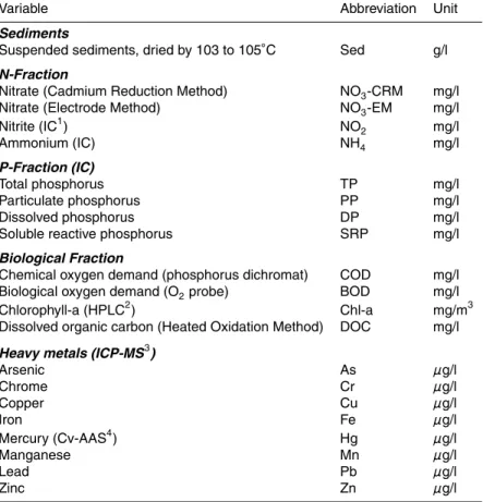
Table 1. Summary of selected surface water quality variables.

Variable Abbreviation Unit

Sediments

Suspended sediments, dried by 103 to 105◦C Sed g/l

N-Fraction

Nitrate (Cadmium Reduction Method) NO3-CRM mg/l

Nitrate (Electrode Method) NO3-EM mg/l

Nitrite (IC1) NO2 mg/l Ammonium (IC) NH4 mg/l P-Fraction (IC) Total phosphorus TP mg/l Particulate phosphorus PP mg/l Dissolved phosphorus DP mg/l

Soluble reactive phosphorus SRP mg/l

Biological Fraction

Chemical oxygen demand (phosphorus dichromat) COD mg/l

Biological oxygen demand (O2probe) BOD mg/l

Chlorophyll-a (HPLC2) Chl-a mg/m3

Dissolved organic carbon (Heated Oxidation Method) DOC mg/l

Heavy metals (ICP-MS3)

Arsenic As µg/l Chrome Cr µg/l Copper Cu µg/l Iron Fe µg/l Mercury (Cv-AAS4) Hg µg/l Manganese Mn µg/l Lead Pb µg/l Zinc Zn µg/l 1 Ion Chromatography. 2

High-Performed Liquid Chromatography.

3

Inductively Coupled Plasma/Mass spectrometry.

(24)

HESSD

3, 2991–3021, 2006

data

M. Rode and U. Suhr

Full Screen / Esc

EGU

Table 2. Important sources of uncertainties of surface water quality data.

Field Sampling Representative Laboratory Load

instruments location sampling analysis calculation Instrument errors Mixing of High spatial Sampling Sampling

large tributaries variation within conservation frequency the cross section

Instrument Point source inputs High temporal variation Sampling transport Sampling period calibration errors (e.g. due to

point source inputs, flood events)

Impoundments, Sampling volume Instrument errors Choice of

dead zones etc. extrapolation method

(e.g. rating curve) Sampling duration Laboratory

(25)

HESSD

3, 2991–3021, 2006

data

M. Rode and U. Suhr

Full Screen / Esc

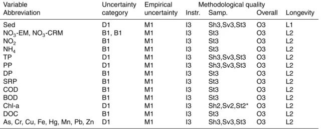
Table 3. Example table, giving information about uncertainty category, type of empirical

uncer-tainty, methodological quality and longevity.

Variable Uncertainty Empirical Methodological quality

Abbreviation category uncertainty Instr. Samp. Overall Longevity

Sed D1 M1 I3 Sh3,Sv3,St3 O3 L1 NO₃-EM, NO₃-CRM B1, B1 M1 I3 St3 O3 L2 NO₂ B1 M1 I3 St3 O3 L2 NH₄ B1 M1 I3 St3 O3 L2 TP D1 M1 I3 Sh3,Sv3,St3 O3 L2 PP D1 M1 I3 Sh3,Sv3,St3 O3 L2 DP B1 M1 I3 St3 O3 L2 SRP B1 M1 I3 St3 O3 L2 COD B1 M1 I3 St3 O3 L2 BOD B1 M1 I3 St3 O3 L2 Chl-a D1 M1 I3 Sh2,Sv2,St2* O3 L2 DOC B1 M1 I3 St3 O3 L2

As, Cr, Cu, Fe, Hg, Mn, Pb, Zn D1 M1 I3 Sh3,Sv3,St3 O3 L2

∗

(26)

HESSD

3, 2991–3021, 2006

data

M. Rode and U. Suhr

Full Screen / Esc

EGU

Table 4. NO−₃-N concentrations, standard deviations and bias for different nitrate concentration

increments obtained in three different laboratories (Standard Methods, 1998).

Increment as NO−₃-N µg/L Standard Deviation µgN/L Bias % Bias µgN/L

290 12 +5.75 +17

350 92 +18.10 +63

2310 318 +4.47 +103

(27)

HESSD

3, 2991–3021, 2006

data

M. Rode and U. Suhr

Full Screen / Esc

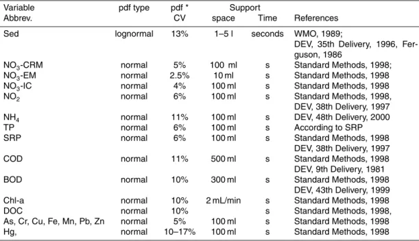
Table 5. Information about error probability distribution type, analytical uncertainties and data

support.

Variable pdf type pdf * Support

Abbrev. CV space Time References

Sed lognormal 13% 1–5 l seconds WMO, 1989;

DEV, 35th Delivery, 1996, Fer-guson, 1986

NO3-CRM normal 5% 100 ml s Standard Methods, 1998;

NO3-EM normal 2.5% 10 ml s Standard Methods, 1998

NO3-IC normal 4% 100 ml s Standard Methods, 1998

NO2 normal 6% 100 ml s Standard Methods, 1998,

DEV, 38th Delivery, 1997

NH4 normal 11% 100 ml s DEV, 48th Delivery, 2000

TP normal 6% 100 ml s According to SRP

SRP normal 6% 100 ml s Standard Methods, 1998

COD normal 11% 500 ml s Standard Methods, 1998

BOD normal 10% 300 ml s Standard Methods, 1998

Chl-a normal 10% 2 mL/min s Standard Methods, 1998

DOC normal 10% s Standard Methods, 1998,

As, Cr, Cu, Fe, Mn, Pb, Zn normal 5% 100 ml s Standard Methods, 1998

Hg, normal 10–17% 100 ml s Standard Methods, 1998

∗

(28)

HESSD

3, 2991–3021, 2006

data

M. Rode and U. Suhr

Full Screen / Esc

EGU

Fig. 1. Chl a longitudinal section of the Elbe sampling survey from Schmilka to Neu Darchau

(29)

HESSD

3, 2991–3021, 2006

data

M. Rode and U. Suhr

Full Screen / Esc

Printer-friendly Version Interactive Discussion 20 40 60 80 100 120 140 160 180 200 10 20 30 40 50 Discharge NH4-N

Distance from left bank (m)

D ischarg e (m 3/ s) 0.00 0.05 0.10 0.15 0.20 Dom Mühlenholz Elb-km 418, 26.05.1993 NH 4-N ( m g/ l)

Fig. 2. NH4-N concentrations and discharge within different segments of the cross section in

(30)

HESSD

3, 2991–3021, 2006

data

M. Rode and U. Suhr

Full Screen / Esc

Printer-friendly Version Interactive Discussion EGU 20 40 60 80 100 120 140 160 180 200 220 10 20 30 40 50 Dom Mühlenholz Elb-km 418, 26.05.1993 Discharge SRP

Di sch arg e (m 3 /s) 0.05 0.06 0.07 0.08 0.09 0.10 SR P ( m g /l)

Fig. 3. Mean SRP-concentrations within the cross section in the Elbe River at location Dom

(31)

HESSD

3, 2991–3021, 2006

data

M. Rode and U. Suhr

Full Screen / Esc

Printer-friendly Version Interactive Discussion 0 20 40 60 80 100 120 140 160 180 200 10 20 30 40 50 Dom Mühlenholz, Elb-km 418, 22.09.1993 Discharge-D Cd

D ischarg e (m 3/ s ) 0.15 0.20 0.25 0.30 0.35 CD ( µ g/ l)

Fig. 4. Mean Cd-concentrations within the cross section in the Elbe River at location

(32)