Uncertainties in river basin data at various support scales ? Example from Odense Pilot River Basin

(1)

HAL Id: hal-00298743

https://hal.archives-ouvertes.fr/hal-00298743

Submitted on 1 Aug 2006

HAL is a multi-disciplinary open access

archive for the deposit and dissemination of sci-entific research documents, whether they are pub-lished or not. The documents may come from teaching and research institutions in France or abroad, or from public or private research centers.

L’archive ouverte pluridisciplinaire HAL, est destinée au dépôt et à la diffusion de documents scientifiques de niveau recherche, publiés ou non, émanant des établissements d’enseignement et de recherche français ou étrangers, des laboratoires publics ou privés.

Uncertainties in river basin data at various support

scales ? Example from Odense Pilot River Basin

J. C. Refsgaard, P. van der Keur, B. Nilsson, D.-I. Müller-Wohlfeil, J. Brown

To cite this version:

J. C. Refsgaard, P. van der Keur, B. Nilsson, D.-I. Müller-Wohlfeil, J. Brown. Uncertainties in river basin data at various support scales ? Example from Odense Pilot River Basin. Hydrology and Earth System Sciences Discussions, European Geosciences Union, 2006, 3 (4), pp.1943-1985. �hal-00298743�

(2)

HESSD

3, 1943–1985, 2006

Data uncertaity at various scale support

for Odense Basin J. C. Refsgaard et al. Title Page Abstract Introduction Conclusions References Tables Figures J I J I Back Close Full Screen / Esc

Printer-friendly Version Interactive Discussion

EGU

Hydrol. Earth Syst. Sci. Discuss., 3, 1943–1985, 2006 www.hydrol-earth-syst-sci-discuss.net/3/1943/2006/ © Author(s) 2006. This work is licensed

under a Creative Commons License.

Hydrology and Earth System Sciences Discussions

Papers published in Hydrology and Earth System Sciences Discussions are under open-access review for the journal Hydrology and Earth System Sciences

Uncertainties in river basin data at

various support scales – Example from

Odense Pilot River Basin

J. C. Refsgaard1, P. van der Keur1, B. Nilsson1, D.-I. M ¨uller-Wohlfeil2, and J. Brown3

1

Geological Survey of Denmark and Greenland (GEUS),Øster Voldgade 10, 1350 Copenhagen, Denmark

2

County of Fyn, Ørbækveij 1400, 5220 Odense, Denmark

3

University of Amsterdam, Nieuwe Achtergracht 166, 1018 NW, Amsterdam, The Netherlands Received: 24 April 2006 – Accepted: 6 June 2006 – Published: 1 August 2006

(3)

HESSD

3, 1943–1985, 2006

EGU

Abstract

In environmental modelling studies field data usually have a spatial and temporal scale of support that is different from the one at which models operate. This calls for a methodology for rescaling data uncertainty from one support scale to another. In this paper data uncertainty is assessed for various environmental data types collected for 5

monitoring purposes from the Odense river basin in Denmark by use of literature in-formation, expert judgement and simple data analyses. It is demonstrated how such methodologies can be applied to data that vary in space or time such as precipitation, climate variables, discharge, surface water quality, soil parameters, groundwater ab-straction, heads and groundwater quality variables. Data uncertainty is categorised 10

and assessed in terms of probability density functions and temporal or spatial autocor-relation functions. The autocorautocor-relation length scales are crucial when support scale is changing and it is demonstrated how the assumption used when estimating the auto-correlation parameters may limit the applicability of these autoauto-correlation functions.

1 Introduction

15

Understanding the uncertainty in environmental data and systems is essential for mak-ing robust and wise water management decisions (Funtowicz and Ravetz, 1990; Beck, 2002; Pahl-Wostl, 2002). Several authors have addressed various aspects of data un-certainty in different disciplines (e.g. Gelhar, 1986; Beven and Binley, 1992; Heuvelink and Burrough, 1993), but so far few attempts have been made to establish a methodol-20

ogy for characterising data uncertainty that is generic and applicable across disciplines. To fill in this gap a new methodology and an associated software tool was developed (Brown, 2004; Brown et al., 2005; Brown and Heuvelink, 2006) and literature surveys were made to support the assessment of uncertainty in different types of data (Van Loon and Refsgaard, 2005).

25

(4)

HESSD

3, 1943–1985, 2006

EGU

of support, both in time and in space. When field data are used for modelling either as input or for comparison with model variables the scale of support of the field data are most often not fully consistent with the scale on which the models operate (Heuvelink and Pebesma, 1999; Refsgaard et al., 1999).

This new data uncertainty assessment methodology and its application to different 5

disciplines are described in several other papers in this HESS Special Issue (Castilla; Dunbar; Nilsson and Refsgaard; Rode and Suhr, 2006; van der Keur and Iversen, 2006; van Loon et al., 2005). Most scientific studies on data uncertainty have been based on data collected for research purposes. The present paper has two main ob-jectives: (1) to test and illustrate the new methodology on different types of data from 10

an ordinary river basin, based on existing data collected for river basin management purposes; and (2) to discuss the fundamental problems arising in connection with such data uncertainty assessment.

2 Methodological considerations

2.1 The HarmoniRiB network of representative river basins 15

Within the EU research project HarmoniRiB (Refsgaard et al., 2005a) data have been collected from eight European river basins. These basins have been selected to en-sure a good coverage across Europe in terms of eco-regions, types of water problems, socio-economic conflicts and amount and quality of existing data. For each of the eight river basins a comprehensive amount of data has been collected and uploaded to the 20

HarmoniRiB database. The data basically include all data that are required to carry out analysis for implementation of the European Water Framework Directive (WFD), i.e. data on climate, rivers, lakes, groundwater, transitional waters, and coastal wa-ters, river basin characteristics and socio-economics. After uploading the data to the database, uncertainty has been assessed and added to the data. The aim of the Har-25

(5)

HESSD

3, 1943–1985, 2006

EGU

and data owners, to provide well documented data for research purposes, suitable for studying the influence of uncertainty on management decisions. The data will be publicly accessible for all research purposes. Thus, scientists may use the data to e.g. assess the appropriateness of models and other tools in relation to the WFD. 2.2 Characterisation of uncertainty – support scale

5

As part of the data processing the HarmoniRiB project partners have characterised and assessed the data uncertainty using the new methodology described by Brown et al. (2005) and using the DUE (Data Uncertainty Engine) software tool (Brown and Heuvelink, 2006). This new methodology has been further elaborated in van Loon et al. (this issue). Tables 1–4 show the key characteristics used to characterise data 10

uncertainty. The terms in these tables are used in Table 5 comprising the key char-acteristics of data uncertainty for the Odense River Basin as assessed in the present paper.

We found it, however, necessary to amend the tables in van Loon et al. (this issue) with characterisation of upscaled time and space support. The reason for this is that 15

many of the data items have a measurement scale support that is considerably smaller than the corresponding variable typically simulated by a model. Let us, as an example, assume that a water quality variable in a river is sampled once per month by taking a bottle of water at a location in the river cross-section. The measurement scale support in this case is a couple of seconds in time and equivalent to the volume of the bottle 20

in space. A river water quality model will typically simulate the concentration as the average for the whole cross-section (unless it is a 3-D river model, which is not com-mon for water quality modelling) and with a time step of somewhere between an hour and a day. The measurement support scales are in this case not compatible with the modelling scales. If the modeller wants to analyse whether the model simulation has 25

an accuracy that is within the range given by the measurement uncertainty it does not, therefore, make sense to compare these data. In such case we have to upscale the field data uncertainty and/or downscale the model scale uncertainty so that the

(6)

tempo-HESSD

3, 1943–1985, 2006

EGU

ral and spatial scales at which uncertainty is considered are the same for field data and modelled variable. The upscaling/downscaling can be done to many different scales depending on the objective of the particular study. If the objective is to assess the flux of the solute on a monthly basis the field data uncertainty could be upscaled to support scales of the cross-section (spatial) and one month (temporal).

5

2.3 Sources of uncertainty

Based on van Loon and Refsgaard (2005) the sources of uncertainty for field data can be characterised as follows:

– Field instruments (instrument errors, instrument calibration errors)

– Laboratory analysis (sample conservation and transport, instrument errors,

in-10

strument calibration errors, laboratory induced uncertainty)

– Model for relating measured values to the variable of interest. This applies in

cases where the measurements are indirect, e.g. when transforming water level measurements to discharge values by use of a rating curve there is uncertainty related to the rating curve.

15

– Representativeness of sample in space (spatial heterogeneity of variable)

– Representativeness of sample in time (temporal variability of variable, sampling

frequency and period, choice of extrapolation method)

The latter two of these sources are those relating to the upscaling from the measure-ment support to a larger scale. In the example above they relate to the upscaling from 20

point scale to cross-sectional scale and from instantaneous to monthly average values. As noted by Rode and Suhr (2006) the sources of uncertainty related to upscaling are often dominant as compared to field instrument and laboratory uncertainty.

(7)

HESSD

3, 1943–1985, 2006

EGU

3 The Odense River Basin

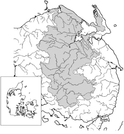
The Island of Fyn covers approximately 3000 km2 of which nearly 80% is cultivated. The Odense river basin covers approximately 1190 km2 of the island (Fig. 1). The present landscape of Fyn was primarily created during the last Glacial Period. The topography is characterised by low rolling hills with three major topographic highs of 5

about 100 m divided by a central lowland. Quaternary deposits up to 150 m thick are exposed at the surface and consist of glacial and interglacial sediments. These de-posits consist primarily of clayey till with lenses and alternating layers of outwash sand, gravel and clay. The most regionally extensive and most heavily exploited aquifer on Fyn consists of Quaternary outwash sands bounded by upper and lower fine-grained 10

deposits.

The annual precipitation and reference evapotranspiration are about 900 mm and 600 mm, respectively. There is a positive precipitation gradient from the northern coast toward the southern boundary of the catchment. The phreatic groundwater table is close to the surface and the low lying areas are generally drained by tile drains. All 15

water supply is based on groundwater abstraction. The two main water resources management problems in the area are (1) groundwater pollution due to point and non-point sources, and (2) eutrophication of Odense Fjord due to nutrient load originating from agricultural areas.

The Odense Pilot River Basin project comprises Denmark’s contribution to the test-20

ing of a number of EU guidance documents relating to implementation of the Water Framework Directive (WFD). All relevant information in this respect is described in Fyns Amt (2003) that also provides a thorough description of the basin, its environ-mental status and the water management issues.

(8)

HESSD

3, 1943–1985, 2006

EGU

4 Description of data and assessment of data uncertainty

In the following sections some of the data collected from the Odense River Basin are described together with the assessed data uncertainty. The data types and the key characteristics of the uncertainty assessment are shown in Table 5. A more detailed description is given in Van der Keur et al. (2006). The reason for selecting these data is 5

that they together illustrate most of the difficulties and fundamental problems we were confronted with when we assessed data uncertainty for the river basin.

4.1 Precipitation data

4.1.1 Data description

Daily values have been collected for seven precipitation stations for the period 1990– 10

2003 (Thomsen and Rosenørn, 2004). Precipitation data are measured by manual readings as accumulated data over 24 h using a Hellman raingauge located 150 cm above the ground.

4.1.2 Uncertainty aspects

The precipitation data are known to be biased, because wetting and wind effects cause 15

the measured data to underestimate the real precipitation (Allerup and Madsen, 1979; Barca et al., 2005). The data can be corrected for this bias by multiplying the mea-sured data by a factor that varies over the year with highest correction factors in winter months where wind speeds are higher and where some of the precipitation falls as snow (Allerup et al., 1998). The average correction factor is 1.21.

20

After removing this bias the uncertainty on the corrected data are still significant. Analyses of point measurements indicate that the uncertainty on the monthly correction factors is between 2% and 11% (Vejen, 2002) implying that uncertainty on daily values are even higher.

(9)

HESSD

3, 1943–1985, 2006

EGU

For precipitation data the measurement support scale is basically a point in space (the area of the gauge is 200 cm3) and a day in time. In all the hydrological models applied for Fyn so far the precipitation data is used as being representative for a model grid or a subcatchment, ranging from a few hundred m to a few hundred km2. As data are used as representative of a given area we have chosen to upscale the spatial 5

support to 170 km2, which in average corresponds to the area covered by one station, if the seven stations are used to estimate the precipitation for the whole basin.

The uncertainty varies both in time and in space. We have chosen an uncertainty model (Table 1) that assumes the data and their uncertainty to be continuous numerical variables that varies in time but are constant in space. The more qualitative character-10

isation of uncertainty of the precipitation data according to type empirical uncertainty (Table 2), methodological quality (Table 3) and longevity (Table 4) are straightforward and shown in Table 5.

Instead of conducting a comprehensive statistical analysis on precipitation data from the Odense catchment, we decided to base the assessments on results from a previous 15

research study in another Danish catchment, Sus ˚a, with similar climatic regime (Allerup et al., 1981, 1982). The advantage of this approach is that these results were based on a sophisticated statistical analysis with much more data than available in our case and that the results are readily available and scientifically published. The disadvantage is that in order to transfer these results to the Odense river basin and to our desired form, 20

we need to make some assumptions that may not all be easy to justify. The critical assumptions and their implications are discussed later in this paper.

In the study by (Allerup et al., 1981, 1982) areal precipitation was estimated for the 800 km2 Sus ˚a catchment on the basis of data from 14 precipitation stations. They found that a normal distribution was applicable. By use of comprehensive statistical 25

analyses considering the effects of spatial and temporal correlations they estimated confidence bounds for the (upscaled) areal precipitation for daily, monthly and annual precipitation as follows:

(10)

HESSD

3, 1943–1985, 2006

EGU

– Standard deviation (monthly values): about 10% of average monthly precipitation – Standard deviation (annual values): about 6% of average annual precipitation

The problem we want to address is now to estimate how accurate one precipitation station would represent the average precipitation over an area of 170 km2. To do that we start by going from the catchment uncertainty for the 800 km2with 14 stations to the 5

uncertainty for one station over 800/14=57 km2. If we assume that the 14 stations are equally spaced and weighted and that data from the 14 stations are spatially indepen-dent, then the standard deviation for one of the stations can be calculated backwards from STD_800km2 = STD_{57 km}2 pN_e_ff (1) 10 where

N_e_ffnumber of independent observations used to calculate the average precipitation over 800 km2

STD_{800 km}2 standard deviation of precipitation over 800 km2 based on N_e_ff

indepen-dent observations 15

STD_{57 km}2 standard deviation of precipitation for one station representing 57 km2

However, due to spatial autocorrelation N_e_ffis less than the number of stations. Spa-tial autocorrelation functions for daily and monthly precipitation are given in (Allerup et al., 1981, 1982). For daily precipitation the spatial autocorrelation over a length corresponding to 57 km2 (7.6 km) is 0.4. By using a standard text book formula for 20

calculating the effective sample size in autocorrelated time series, e.g. Salas (1993), with 14 stations and a correlation coefficient of 0.4, N_e_ff can in this case be calculated to 12.5. By rearranging Eq. (1) STD_57km2 is calculated to

p

(11)

HESSD

3, 1943–1985, 2006

EGU

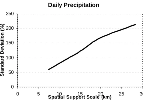
This implies that by upscaling the spatial support of precipitation data from representing 57 km2(7.6 km) to representing 800 km2(28 km) the standard deviation increases from 60% to 210%. By making the same calculation for different number of stations the relationship shown in Fig. 2 appears. For the case of the Odense river basin we want to upscale the support to 170 km2 (13 km) which then is seen (Fig. 2) to result in a 5

standard deviation of about 105% of the average daily precipitation.

For monthly values the spatial autocorrelation is larger. Using the correlation func-tion for monthly values shown in Allerup et al. (1981) the relafunc-tionship between spatial support and standard deviation becomes as shown in Fig. 3. For the case of Odense river basin the standard deviation upscaled to a spatial support of 170 km2 (13 km) is 10

seen to be 19%. If the correlation structure for annual values is similar to the monthly correlation the standard deviation for annual values upscaled to 170 km2(13 km) would be 11%. If the annual correlations are higher than the monthly values, which is a rea-sonable assumption, the standard deviation for the annual values would become less than 11%.

15

For an uncertainty category B1 (varies in time, not in space) we also need to estimate an autocorrelation function and the associated parameter values. We could not find much relevant information on this. Therefore we assumed an exponential shape of the autocorrelation function. The parameter to estimate is then the autocorrelation length scale. The review of Barca et al. (2005) does not provide information on this parameter. 20

Willems (2001) found that there was hardly any autocorrelation in hourly and half-daily data from Belgium. Allerup et al. (1981) in their statistical analyses of temporal and spatial correlation found temporal autocorrelation on daily data in the order of a few days. We have therefore assumed a parameter value for the autocorrelation length scale of 2 days.

25

With this autocorrelation length scale of 2 days the standard deviation of monthly and annual values can be estimated and compared to the figures derived above. If the monthly average precipitation is estimated from daily values then the standard devia-tion on the monthly mean value can be estimated form the standard deviadevia-tion on the

(12)

HESSD

3, 1943–1985, 2006

EGU

daily data (105%) and the effective sample size (30 reduced to 30/2 due to temporal au-tocorrelation) to (30/2)−1/2 105%=27%. This is somewhat larger than the 19% derived from Fig. 3. A similar calculation for annual values results in (365/2)−1/2 105%=8%, which is somewhat less than the 11% given above. The autocorrelation structure in re-ality, as also reflected in the statistical model developed by Allerup et al. (1981, 1982), 5

is truly spatio-temporal, while the B1 model used here is only temporal. We have then tried to compensate for this lack by using the results from Allerup et al. (1981) to derive temporal autocorrelation models for different spatial scales. The above calculation is a check illustrating to which extent our relatively simple uncertainty model can reflect the spatio-temporal autocorrelation structure in the much more comprehensive model 10

by Allerup et al. (1981). The comparisons show that there are clear limitations in our simple model and that is should be used with care. However, considering the crude assumptions made, the figures match reasonably well indicating that there are no ma-jor discrepancies in the uncertainty model and that if it is used to generate random samples of daily data then the uncertainties on monthly and annual basis will be of the 15

right order of magnitude.

4.2 Climate data

Daily values of temperature, wind direction, wind speed, relative humidity and solar radiation have been collected for one climate station that is located at the same place 20

as one of the seven precipitation stations. The data are described in Thomsen and Rosenørn (2004). The climate station was modernised in 2001. The instrumentation of the stations is listed in Table 6. The daily values are aggregate values based on continuously recordings. The daily potential evapotranspiration is calculated by means of a modified Makkink formula (Scharling, 2001) where the variables are aggregated to 25

(13)

HESSD

3, 1943–1985, 2006

EGU

The climatic data on temperature, relative humidity, wind direction and speed and so-lar radiation have a measurement time support of 1 day obtained from aggregated continuous measurements. The uncertainty category is for all variables is B1 (varies temporally, not in space) and the empirical uncertainty, methodological quality and 5

longevity is as for precipitation (Barca et al., 2005), except for air temperature and rel-ative humidity where the overall method is evaluated as O4, i.e. approved standard in well established discipline. As the potential evapotranspiration is calculated and not di-rectly measured, the methodological quality is O2, as the method is accepted, but with limited consensus on reliability. Plauborg et al. (2002) reported that potential evapo-10

transpiration calculated using the Makkink formula (Makkink, 1957) could be up to 10% overestimated (Table 5). The measurement space support for air temperature, relative humidity and solar radiation is the sensor area of about 10 cm2. Often climate data are used to represent larger areas. For instance Nielsen et al. (2004) used climate variables from one stations to represent the entire 800 km2Odense Basin. Therefore, 15

it would b useful to apply an upscaled support scale of 800 km2. As we have no infor-mation on uncertainty when this space support is rescaled, the measurement space support in maintained in Table 5. The assessed uncertainties are based on information in Barca et al. (2005). The autocorrelation function is assumed to be of the exponential type with a length scale of 2 days as for precipitation.

20

4.3 Discharge data 4.3.1 Data description

There are 10 river gauging stations in the basin. At these stations water levels are measured by continuous recordings. Discharge measurements are made manually by use of current meters at regular (approximately monthly) intervals and rating curves 25

(14)

HESSD

3, 1943–1985, 2006

EGU

form and growth of weed. The water level recordings are transformed to average daily water levels, which then are converted to average daily discharges by use of a time varying rating curve. Data are collected for the period 1990–2000.

According to information from the organisation (NERI) responsible at a national level for 5

discharge measurements a typical uncertainty (standard deviation) on daily discharge data is in the order of 10%, while the uncertainty on annual average flows is about 5% (Refsgaard et al., 2003). This is also the order of magnitudes indicated in (Goodwin, 2005).

The uncertainty characteristics of the discharge, according to the methodology de-10

scribed by van Loon et al. (2006) are similar to those of the precipitation data, namely an uncertainty model that assumes variation in time but not in space (B1) and empirical uncertainty, methodological quality and longevity as shown in Table 5.

The measurement support in space is the river cross-section (indicated as 1–20 m2 in Table 5), while the time support is one day (it is daily average water levels that are 15

converted to daily discharges). The uncertainties on the data are assumed to be zero-mean, Gaussian, with a standard deviation of 10% of the measured discharge.

The difficult issue here is to assess the temporal autocorrelation. In Table 5 it is given as an exponential function with a temporal length scale of 90 days. The review made by Goodwin (2005) does not provide much support in this respect. The assumption 20

of an exponential function is therefore somewhat arbitrary, although an exponential correlation structure is common in time-series analysis (e.g. Sivapalan and Bl ¨oschl, 1998). The reasoning behind the 90 days as temporal length scale is related to the uncertainty of 10% and 5% on daily and annual flows, respectively. If the daily flows were assumed not to be correlated (length scale = 0 days) the uncertainty on the 25

(15)

HESSD

3, 1943–1985, 2006

EGU

values (STD_{daily flow}) as follows:

STD_{annual flow}=

STD_{daily flow} √

N

(2)

where N is the number of observations. With N=365 and STD_{daily flow}=10%, STD_{annual flow} becomes 0.5% which is a factor 10 too low. If we consider autocorre-lation, N can be considered as the equivalent number of independent observations. If 5

we for instance have N=4 we get STD_{annual flow}=5%. N=4 can be interpreted as a year information content equivalent to four independent observations or in other words that the average length scale is in the order of 90 days.

This backwards calculation give us some kind of consistency between uncertainty on daily and annual flow. However, it can be argued that the “uncertainty model” in 10

this case is too simplistic and will lead to wrong conclusions for many applications. In reality the uncertainties most likely contains both a bias on the expected value and an autocorrelation on the residual. The bias could be related to representativeness of the current meter profiles and the shape of the rating curve. If the data is biased on one day they are also likely to be biased on other days, which will increase the correlation 15

and the variance of the combined uncertainty. We do not know how the uncertainty in reality is decomposed into bias and partially correlated variability, but this combination can explain that we by the backwards calculation arrive at an autocorrelation length scale that is much larger than one would assume if only considering instrument and other measurement errors. A further discussion on the applicability and limitations of 20

the above results are given in the final section of the paper. 4.4 Tot N in streams

The concentration of Total nitrogen (Tot N) is monitored at some of same river gauging stations where water levels are also measured. Daily data have been collected from 4 25

(16)

HESSD

3, 1943–1985, 2006

EGU

stations for the period 1990–2000. The samples for Tot N analyses are taken as time proportional sampling aggregated over one day. The samples are taken at a point in the river, which is indicated by a space support of 100 ml in Table 5.

We have decided to upscale the space support from a point in the river (100 ml) to the 5

river cross-section. This implies that we can consider the uncertainty to be composed of two elements: (a) one related to the measurement at point scale (sampling, instru-ment, laboratory procedures, etc.) and (b) the other related to the representativeness of the point (100 ml) to characterise average cross-sectional concentration.

The statistical distribution is assumed to be Gaussian, as recommended by Rode 10

and Suhr (this issue). Rode and Suhr (this issue) furthermore suggest that the instru-ment and measureinstru-ment uncertainty for point samples have a coefficient of variation of 5%. The main difficulty in our case is therefore to assess how upscaling of space sup-port from point to cross-sectional area affects the uncertainty. This can be done in dif-ferent ways. If sufficient data is available, or if sufficient assumptions can be made, on 15

the spatio-temporal correlation structure within the cross-section, the uncertainty can be assessed through spatio-temporal block kriging (Heuvelink and Webster, 2001). We had no data (only one sample point) or information to justify any assumptions to sup-port this. Instead we have relied on experience on how mixing or lack of mixing within a cross-section affects variation of concentrations across a profile. Based on data and 20

recommendations made by Rode and Suhr (this issue) we assume that the uncertainty of a single point to represent average value of an entire cross-section corresponds to a factor of 2. By multiplying the coefficient of variation for instruments/measurements (5%) with this representativeness factor the uncertainty at a cross-sectional scale is estimated to be 10%.

25

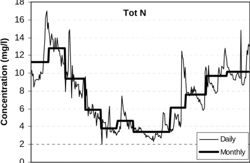
The time series of daily data allows analysis of how representative a daily value is for the monthly average, or in other words an upscaled temporal support of the uncertainty to one month. Figure 4 shows daily and monthly average concentrations for one station

(17)

HESSD

3, 1943–1985, 2006

EGU

for one year. The concentration of Tot N is seen to have a clear seasonal pattern with relatively slowly varying daily fluctuations on top. The variability of daily values within a month can be characterised by the coefficient of variation, i.e. the standard deviation divided by the mean monthly value. The average coefficient of variation for the 12 months shown in Fig. 4 can be calculated to 0.22 implying that the average error of 5

using a daily value instead of the mean monthly value is 22%.

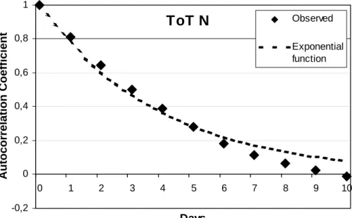
A time series analysis of the Tot N values for the whole period 1990–2003 resulted in the autocorrelogram shown in Fig. 5. Before calculating the autocorrelogram the seasonal pattern was removed by subtracting the monthly mean values from the daily values. The autocorrelation is seen to fit nicely to an exponential function with a time 10

scale of 4 days. The autocorrelation is therefore assumed to follow an exponential distribution with a correlation length scale of 4 days (Table 5).

4.5 Tot P in streams

The concentration of Total phosphorous (Tot P) is monitored at some of same river 15

gauging stations where also water levels are measured. Daily data have been col-lected from 4 stations for the period 1990–2000. Samples for Tot P are taken time proportionally in small volumes with a space support of 100 ml. Time proportional measurements are aggregated to 1 day. Therefore the time support is indicated as 1 day and the space support as 100 ml in Table 5.

20

The analysis leading to the uncertainty characteristics are similar to those for N Tot. The only difference is that the uncertainty related to instruments and laboratory analy-sis are assumed to be characterised by a standard error of 6% instead of 5% for N Tot following recommendations from Rode and Suhr (this issue).

(18)

HESSD

3, 1943–1985, 2006

EGU

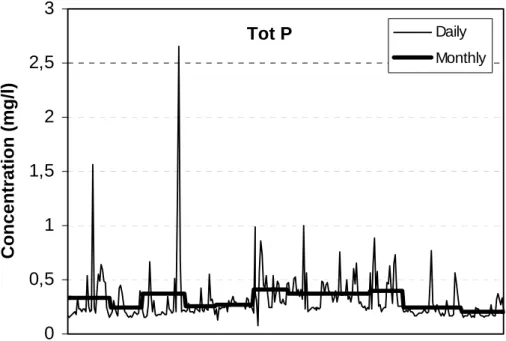
Figure 6 shows the variability of daily Tot P values within a month. In contrary to the Tot N data shown in Fig. 4, the concentration of Tot P does not show a seasonal pattern, and the daily concentrations are much more erratic. The average coefficient of variation within a month for the Tot P data is 0.51 which is considerably higher than the 0.22 for Tot N. This more erratic behaviour is consistent with the much lower autocorrelation 5

length scale of one day for Tot P (Fig. 7).

4.6 Heavy metals in streams

The concentration of about 10 compounds of heavy metals is monitored at some of same river gauging stations where also water levels are measured. Data have been 10

collected from 2 stations and 29 compounds for the period 1990–2000. Samples for heavy metals are taken as instantaneous samples in small volumes with a space sup-port of about 100 ml. Therefore the time supsup-port is indicated as 10 s and the space support as 100 ml in Table 5. Sampling is made approximately once per month.

4.6.2 Uncertainty aspects 15

Like for the case of Total N in streams we have decided to upscale the space sup-port from a point in the river (100 ml) to the river cross-section. In addition, we have upscaled the temporal support from an instant (10 s) to one month. This implies that we, in addition to instrument and measurement uncertainty, need to include the uncer-tainty of the point sample in representing average cross-sectional conditions and of the 20

instantaneously sampled data to representing monthly average concentrations. The statistical distributions for the uncertainties, including the autocorrelation, are assumed to be as for the data type “N-Total in streams”. The only difference is the standard error that here is assumed to be 20% instead of 10%. The rationale for the 20% is as follows:

(19)

HESSD

3, 1943–1985, 2006

EGU

– The instrument/measurement uncertainty is assumed to be 5%. This is based on

Rode and Suhr (this issue)

– The spatial upscaling from point to cross-section is assumed to result in an

in-crease of the uncertainty with a factor 2 as for the case of “N-Total in streams”.

– The temporal upscaling from 10 s to 1 month is assumed to result in an increase

5

of the uncertainty with a factor 2. This factor is partly justified by data. The variation of daily data on Tot N and Tot P (Figs. 4–5) show that the coefficient of standard deviation during a month divided by the mean value of the month was in average 0.22 for Tot N and 0.51 for Tot P. This coefficient of variation can be seen as a measure of the uncertainty of a daily value to be representative for a 10

monthly value. As Tot P data are likely to be more representative for most heavy metals in its behaviour, because it depends more on suspended sediments than Tot N does, the factor for the Tot P is used. Unfortunately, no similar data exist for variations within a day. Assuming that this is the same order of magnitude we arrive at the uncertainty factor of 2.

15

The autocorrelation is here assumed to follow an exponential distribution with a cor-relation length scale of one day. This assumption is based on the data from Tot P, but we have no specific data on heavy metals to support this assumption which therefore is questionable. However, with an upscaled temporal support of one month a correlation length scale of one day implies that the monthly data are considered independent, and 20

hence the autocorrelation function is of no practical importance.

4.7 Pesticides and organic compounds in streams 4.7.1 Data description

The concentrations of about 29 pesticides and other organic compounds are monitored at two of the same river gauging stations where also water levels are measured. Data 25

(20)

HESSD

3, 1943–1985, 2006

EGU

have been collected from the two stations for the period 1998–2003. Samples are taken as instantaneous samples in small volumes. Therefore the time support is indicated as 10 s and the space support as 100 ml in Table 5. Sampling is made approximately once per month.

The analysis leading to the uncertainty characteristics are similar to those for heavy metals. The only difference is that the uncertainty related to instruments and laboratory analysis are assumed to be characterised by a standard error of 10% instead of 5% for heavy metals following recommendations from Rode and Suhr (this issue). The autocorrelation function is assumed identical to the one for heavy metals discussed 10

above.

4.8 Groundwater data

For the Odense catchment 116 groundwater bodies at various depths have been iden-tified, mapped and monitored for drinking water purposes. Water abstraction data from 15

168 wells are recorded on a yearly basis. Groundwater head is monitored by means of automated datalogger recordings from some wells and by manual sampling from other wells in a dense network. Most groundwater bodies are monitored for nitrate, phosporus, heavy metals and pesticide concentrations as well as physical-chemical properties, like pH, temperature and alkalinty. Sampling for compounds and physical 20

properties is usually on a yearly basis and the measurement space support is 100 ml. Water quality has since 1990 been measured yearly from 2255 wells with 2615 intakes of which 1811 are connected to groundwater bodies (Fyns Amt, 2005).

(21)

HESSD

3, 1943–1985, 2006

EGU

Well abstraction data are usually very reliable and uncertainties due to instrument accu-racy are low. However, data may be uncertain with respect to the origin of abstractions due to the location of filters relative to assumed boundaries between different aquifers. We have characterised the uncertainty by a normal distribution with zero mean and a 5

standard deviation of 2% of the abstracted volumes (Table 5). The uncertainties of the annual data are assumed to be independent in time.

The spatial support scale for groundwater head observations are upscaled from a point to 0.5×0.5 km2, because this is a common grid scale for regional groundwater modelling (Henriksen et al, 2003). The temporal support scale is upscaled from a point 10

in time (10 s) to one year for the manual observations, while it is kept at the 10 s for the automatically recorded data. Inspired by the methodology described in Henriksen et al. (2003) the uncertainty of one observation to represent 0.25 km2at 10 s or one year can be assumed to be composed of the following independent sources of uncertainty:

– measurement errors: 0.1 m

15

– scaling errors due to hydraulic head gradient over the 500 m grid and uncertainty

on where in the grid the observation well is located: 0.75 m

– uncertainty due to geological heterogeneity: 1.0 m

– non-stationarity, i.e. head fluctuations over a year: 0.5 m (this becomes 0 m in

case of automatic readings and 10 s support scale) 20

Using the error propagation equation the uncertainty can then be calculated to 1.35 m and 1.25 m for the manual and automatically recorded data respectively. We have no information on the autocorrelation function for the groundwater head data (Table 5).

No data is available on probability density and autocorrelation functions for physical-and chemical properties. Measurements of physical physical-and chemical properties may be 25

(22)

HESSD

3, 1943–1985, 2006

EGU

may be taken from a mixture of water from near-surface and deeper aquifers dependent on the filter position and geologic structure around the filter. Usually, counties monitor sample measurements for anomalies with regard to discontinuities in data over time as a means of data quality assurance (Copenhagen County , personal communication). Time between samples is dependent on the location (depth) of the reservoir and for 5

routinely monitoring purposes the range is usually between 1 month and 1 year for surface near- and deep-groundwater respectively.

4.9 Soil data

Soil texture for Fyn is measured at 20 cm depth in 3619 points. The texture class is 10

subdivided in clay, silt, fine sand and coarse sand. Furthermore soil organic matter (SOM), CaCO₃content and a colour code are registered. Coordinates of all point are provided in UTM coordinates. Soil hydraulic properties are not included and must be estimated from pedotransfer functions.

Uncertainty in soil (physical) data arises from the spatial and temporal variability of environmental variables, from sampling procedures in the field, and from analysis in the laboratory. Soil variability is the product of soil-forming factors operating and interacting over a range of spatial and temporal scales. The uncertainty characteristics listed in Table 5 are in accordance with the recommendations in van der Keur and Iversen (this 20

issue). Here it is only noted that the soil data, in contrary to the other data types in Table 5 vary in space, but not in time, making the measurement and upscaled time supports irrelevant in this case.

The measurement space support for soil samples taken in the field are typically in the order of magnitude of 100 cm3. Mulla and McBratney report ranges in coefficient 25

(23)

HESSD

3, 1943–1985, 2006

EGU

of variation of 3–37% and 16–53% for sand- and clay content respectively. This is translated to 25% and 40% in Table 5 where 30% is assumed for silt content. Spatial autocorrelation lengths for soil texture are reviewed in van der Keur and Iversen (this is-sue). For clay-, silt- and sand content, Neuman and Wierenga (2003) found correlation lengths ranging from 20–33 m, 20–26 m and 20–35 m respectively, fitted to spherical 5

models. Soil organic matter Hansen et al. (1999) estimate the standard error to be 25% and Kristensen et al. (1995) fit an exponential model to the data with a range of 34–45 m. For CaCO3 content the standard error is 10% and the variogram model of the exponential type with a range of 30 m (Kristensen et al., 1995). This is shown in Table 5.

10

5 Discussion and conclusions

5.1 Critical assumptions

In order to make the above uncertainty assessments many assumptions had to be made. Many of these assumptions used in the expert judgements are based on gen-eral knowledge from literature or on regional knowledge from nearby catchments and 15

the validity of these assumptions to the Odense River Basin can, and should, be ques-tioned. It would no doubt have been better to have more detailed local data, which would have been possible in an experimental research catchment. However, when making assessment of data uncertainty in real life basins where “only” data from rou-tine monitoring programmes exist, it is often necessary to make such assumptions and 20

simplified expert judgements. Odense river basin is one of the so-called Pilot River Basins used as testing ground for guidelines for the EU Water Framework Directive. And it is probably the basin among the about 15 Pilot River Basins with the best data availability. So for most other basins it will be necessary to make even more assump-tions than we have done here.

25

(24)

HESSD

3, 1943–1985, 2006

EGU

– The most critical assumption is probably that we have assumed data to vary either

spatially (C1) or temporally (B1), whereas many data in reality varies both in time and space (D1). The way we circumvented this assumption for precipitation data was to upscale temporally varying data to a certain scale of support. This may, as discussed above, lead to inconsistency when these data are then aggregated 5

from daily to monthly or annual values.

– The assumptions made on spatial and temporal autocorrelation length scales

have generally not been much supported by local data and are therefore very uncertain. These autocorrelation length scales are crucial when the data are up-scaled in either space or time.

10

– In case of sampling from a river cross section, measurements vary across the

cross-section and over time. Usually one measurement is taken for the entire cross-section and assumed representative as no information exists on the spatial distribution. Again we rely on experience from literature and transfer it to our own case. In the rare event of having knowledge on the spatio-temporal behaviour of 15

the variable at hand, spatio-temporal geostatistics may be applied for upscaling to the cross-section support scale. In this case the similar assumptions apply as for the spatial- or temporal case.

– We use data from Sus ˚a instead of Odense for precipitation. This is probably a

less critical assumption as compared to many of the other ones, because it is 20

based on a very comprehensive statistically based research study with a much data in the Sus ˚a basin, and because the climatic regimes do not differ very much between the two basins.

In spite of these simplistic and crude assumptions we see no other realistic option if uncertainty assessments should be carried out in ordinary river basins as an integrated 25

part of the water resources management. The only alternative in most cases would in practise be to make no uncertainty assessments at all. And we consider this a very

(25)

HESSD

3, 1943–1985, 2006

EGU

poor alternative. One of the important aspects of uncertainty assessments is to make uncertainty aspects a recognised factor in the whole water management process.

Although data uncertainty is only one source of uncertainty in water resources man-agement, and some times even not the most important one (Refsgaard et al., 2005; Højberg and Refsgaard, 2005; Waetzold, 2000) it is a source of uncertainty which is 5

relatively easy to handle in statistical terms and therefore for many people easier to comprehend than many other sources of uncertainty that can only be characterised qualitatively. The difficulty of handling uncertainty in an objective manner has often been a barrier with the result that uncertainty has been neglected in the management process. As we consider uncertainty as a very important element in water resources 10

management it is therefore important to encourage water managers to be aware of uncertainty and include it some way or the other in the management process. In this perspective assessments of data uncertainty may in some cases be an eye opener il-lustrating the importance of uncertainty, and therefore relatively simple methodologies like the ones used in the present paper are important.

15

5.2 Limitations in applicability of our simplistic uncertainty models

The critical assumptions leading to the uncertainty models for the various data types have some implications in terms of limitations of applicability.

Let us as an example look at the discharge data where we assessed that an autocor-relation length scale of 90 days were required in order to match the expert information 20

that uncertainty on daily and annual discharge values could be characterised by stan-dard deviations of 10% and 5 % of the daily and annual mean values, respectively. By doing so we ensured that if daily discharge time series were generated then the annual flow values would have the right order of magnitude of uncertainty. A simple analysis of the discharge time series would show that the autocorrelogram would not have an 25

autocorrelation length scale of 90 days. It would probably rather be in the order of a few days. Thus, if the discharge series should be used to analyse something related to peak flows, generation of time series with a length scale of 90 days would lead to very

(26)

HESSD

3, 1943–1985, 2006

EGU

wrong results. If we had used a length scale suitable for generation of short term phe-nomena like floods, the uncertainty would not be able to preserve the correct level of uncertainty for mean annual flows. Similarly the 90 days length scale for discharge can not be used to assess the necessary sampling frequency. By assuming the uncertainty model valid for such purpose one might get the idea that much more than four samples 5

per year would be waste of money. This is of course not the case. This illustrates that the simple models can be calibrated to fit certain phenomena, but if the uncertainty model is intended to be used for something outside the calibration base, then it can not be assumed valid and this extrapolation might lead to very biased results.

Another illustration of the same problem is the autocorrelation function for river wa-10

ter quality variables, where the autocorrelation length scales were assessed from time series analysis to be 1–4 days. The key sources of uncertainty for water quality at cross-sectional scale are (a) instrument and laboratory calibration and practise and (b) representativeness of point sample at cross-sectional scale. The time scales derived from the autocorrelation analysis only considers the first of these sources, which can 15

be assumed unbiased. The second uncertainty source is very likely to be biased. If the sampling point has a lower concentration than the cross-sectional average concentra-tion on one day it is also likely to be lower on another day. We do not know the average bias. Therefore we can only assume an expected mean of this uncertainty of zero, but the uncertainty will be consistently either positive or negative. What we have done is 20

to aggregate these two uncertainty terms in one term. By doing so the aggregated autocorrelation length scale is likely to be much larger than the 1–4 days. This implies that use of an autocorrelation function with time scales of a few days to generate time series of water quality variables may be appropriate if the purpose of a study is to look at short term variations, but if such series are used to analyse annual mean values of 25

concentrations the uncertainty on the annual values will be severely underestimated. The reason for this lack of universal applicability of the uncertainty models is that it is only an approximation within a small window of the true spatio-temporal autocorrelation structure. A simple model can be thought of as an approximation like a tangent is

(27)

HESSD

3, 1943–1985, 2006

EGU

a linear approximation to a non linear curve. The approximation is very good near its point of derivation, but will become less and lees accurate the further away from this point we move. Therefore an important conclusion is that we have to be careful when using the uncertainty models. They are in a way only valid for certain types of applications, and it is necessary to understand the assumptions and limitations in order 5

to use them correct.

5.3 Selection of upscaled spatial support for uncertainty

Why do we have to upscale the spatial and temporal support? Could we not just assess the uncertainty at the support scale of measurements and then leave the remaining upscaling to the modellers or other users of the data uncertainty? In principle we could 10

stop at the measurement scale. But then we would have to provide a detailed spatio-temporal autocorrelation function in order to enable future users of the uncertainty information to make a suitable upscaling. This would from an ideal, theoretical point of view be preferable. However in practise there are two problems with such approach:

– We do not know the detailed spatio-temporal autocorrelation function. And it

15

would be a function where the assumptions on second-order stationarity in time and space are severely violated.

– Most standard software tools can not deal with such sophisticated spatio-temporal

autocorrelation functions. For instance, the DUE (Brown and Heuvelink, 2005) can only treat uncertainty autocorrelation functions that describe variation in either 20

time or in space, not both in time and space at the same time.

The choice of which upscaled spatial support to use is a subjective decision depend-ing on the intended application of the data and their uncertainty. To illustrate this let us consider the case of river water quality data, where we decided to upscale the data uncertainty from a point sample to the river cross-section. In a case where a model 25

(28)

HESSD

3, 1943–1985, 2006

EGU

the sampling length scale (e.g. 10 cm) an upscaling to cross-sectional support is not relevant (if the exact xyz location of each sample is known and more or less matches the cross-sectional grid). But for the more common case of 1-dimensional river mod-elling which operates with cross-sectional average concentrations the upscaled value is the one of interest in modelling. It is essential to ensure that there is no mismatch 5

of support scale between field data and modelling when using the field data either as direct input to the model or as calibration or validation data.

Acknowledgements. The present work was carried out within the project “Harmonised Tech-niques and Representative River Basin Data for Assessment and Use of Uncertainty Informa-tion in Integrated Water Management” (www.harmonirib.com), which is partly funded by the EC

10

Energy, Environment and Sustainable Development programme (Contract EVK1-2002-00109).

References

Allerup, P. and Madsen, H.: Accuracy of point precipitation measurements, Danish Meteorolog-ical Institute, ClimatologMeteorolog-ical papers no 5, 1979.

Allerup, P., Madsen, H., and Riis, J.: Nedbør. Rapport SUS ˚A H1, Dansk Komite for Hydrologi,

15

90 pp. (in Danish), 1981.

Allerup, P., Madsen, H., and Riis, J.: Methods for Calculating Areal Precipitation applied to the Sus ˚a catchment, Nordic Hydrol., 13(5), 263–278, 1982.

Allerup, P., Madsen, H., and Vejen, F.: Standardværdier (1998) af nedbørskorrektioner, Teknisk Rapport 98-10, Danmarks Meteorologiske Institut (in Danish), 1998.

20

Barca, E., Passarella, G., and Vurro, M.: Climatological data, in: Guidelines for assessing data uncertainty in river basin management studies, edited by: van Loon, E. and Refsgaardm J. C., HarmoniRiB report,http://www.harmonirib.com, 2005.

Beck, M. B.: Environmental Foresight and Models, A manifesto, Elsevier, Oxford, 2002. Beven, K. and Binley, A. M.: The future of distributed models, model calibration and uncertainty

25

predictions, Hydrol. Processes, 6, 279–298, 1992.

Brown, J. D.: Knowledge, uncertainty and physical geography: towards the development of methodologies for questioning belief, Transactions of the Institute of British Geographers, 29(3), 367–381, 2004.

(29)

HESSD

3, 1943–1985, 2006

EGU Brown, J. D., Heuvelink, G. B. M., and Refsgaard, J. C.: An integrated framework for assessing

and recording uncertainties about environmental data, Water Sci. Technol., 52(6), 153–160, 2005.

Brown, J. D. and Heuvelink, G. B. M.: Data Uncertainty Engine (DUE) User’s Manual, University of Amsterdam,http://www.harmonirib.com, 2006.

5

Funtowicz, S. O. and Ravetz, J.R.: Uncertainty and Quality in Science for Policy, Kluwer, Dor-drecht, 1990.

Fyns Amt.: Odense Pilot River Basin. Provisional Article 5 Report pursuant to the Water Frame-work Directive, Fyn County, 132 pp.,http://odenseprbuk.fyns-amt.dk, 2003.

Fyns Amt.: Kortlægning af grundvandsressourcerne – status for vandressourcekortlægningen

10

2005, Miljø- og Arealafdelingen, Fyn Amt (in Danish), 2005.

Gelhar, L.: Stochastic subsurface hydrology. From theory to applications, Water Resour. Res., 22(9), 135–145, 1986.

Goodwin, T.: Discharge Data, in: Guidelines for assessing data uncertainty in river basin management studies, edited by: van Loon, E. and Refsgaard, J. C., HarmoniRiB report,

15

http://www.harmonirib.com, 2005.

Hansen, S., Thorsen, M., Pebesma, E., Kleeschulte, S., and Svendsen, H.: Uncertainty in simulated leaching due to uncertainty in inputs, Soil Use Manage., 15, 167–175, 1999. Henriksen, H. J., Troldborg, L., Nyegaard, P., Sonnenborg, T. O., Refsgaard, J. C., and Madsen,

B.: Methodology for construction, calibration and validation of a national hydrological model

20

for Denmark, J. Hydrol., 280, 52–71, 2003.

Heuvelink, G. B. M. and Burrough, P. A.: Error propagation in cartographic modelling uisng Boolean logic and continous classification, Int. J. Geographical Inf. Sci., 7(3), 231–246, 1993. Heuvelink, G. B. M. and Pebesma, E. J.: Spatial aggregation and soil process modelling,

Geo-derma, 89, 47–65, 1999.

25

Heuvelink, G. B. M. and Webster, R.: Modelling soil variation: past, present, and future, Geo-derma, 100, 269–301, 2001.

Højberg, A. L. and Refsgaard, J. C.: Model Uncertainty – Parameter uncertainty versus con-ceptual models, Water Sci. Technol., 52(6), 177–186, 2005.

Makkink, G. F.: Ekzameno de la formula de Penman, Neth. J. Agric. Sci., 5, 290–305, 1957.

30

Refsgaard, J. C., Kern-Hansen, C., Plauborg, F., Ovesen, N. B., and Rasmussen, P.: Ferskvan-dets kredsløb og tidslige variationer, in: FerskvanFerskvan-dets kredsløb, NOVA 2003 Temarapport, edited by: Henriksen, H. J. and Sonnenborg, A., Geological Survey of Denmark and

(30)

Green-HESSD

3, 1943–1985, 2006

EGU land (in Danish), 2003.

Pahl-Wostl, C.: Towards sustainability in the water sector – the importance of human actors and processes of social learning, Aquatic Sci., 64, 394–411, 2002.

Plauborg, F., Refsgaard, J. C., Henriksen, H. J., Blicher-Mathiesen, G., and Kern-Hansen, C.: Vandbalance p ˚a mark- og oplandsskala, DJF rapport, Nr.70. (in Danish), 2002.

5

Refsgaard, J. C., Thorsen, M., Jensen, J. B., Kleeschulte, S., and Hansen, S.: Large scale modelling of groundwater contamination from nitrogen leaching, J. Hydrol., 221(3–4), 117– 140, 1999.

Refsgaard, J. C., Nilsson, B., Brown, J., Klauer, B., Moore, R., Bech, T., Vurro, M., Blind, M., Castilla, G., Tsanis, I., and Biza, P.: Harmonised Techniques and Representative River Basin

10

Data for Assessment and Use of Uncertainty Information in Integrated Water Management (HarmoniRiB), Environ. Sci. Policy, 8, 267–277, 2005a.

Refsgaard, J. C., van der Sluijs, J. P., Højberg, A. L., and Vanrolleghem, P. A.: Uncertainty Analysis. Harmoni-CA Guidance No. 1., 46 pp., Downloadable fromhttp://www.harmoni-ca.

info, 2005b.

15

Rode, M. and Suhr, U.: Uncertainties in selected surface water quality data, Hydrol. Earth. Syst. Sci. Discuss., (This issue), in press, 2006.

Salas, J. D.: Analysis and modelling of hydrologic time series, in: Handbook of Hydrology, edited by: Maidment, D., Mcgraw-Hill, Chapter 19, 1993.

Scharling, M.: KLIMAGRID DANMARK – Sammenligning af potential fordampning beregnet

20

udfra Makkinks formel og den modificerede Penman formel, Technical Report 01–19, Danish Meteorological Institute (in Danish), 2001.

Sivapalan, M. and Bl ¨oschl, G.: Transformation of point rainfall to areal rainfall: Intensity-duration-frequency curves, J. Hydrol., 204, 150–167, 1998.

Thomsen, L. and Rosenørn, S.: Daily Climate Data to Odense Fjord Pilot River Basin 1990–

25

2003, DMI Technical Report No. 04–24, Danish Meteorological Institute, 2004.

Van der Keur, P., M ¨uller-Wohlfeil, D.-I., Nilsson, B., and Refsgaard, J. C.: Description of data uploaded to HarmoniRiB database from the Odense catchment and description of method-ology for assessment of data uncertainty, in: Harmonirib River Basin Data Report, edited by: Passarella, G.,http://www.harmonirib.com, 2006.

30

Van der Keur, P. and Iversen, B. V.: Uncertainty in soil physical data at river basin scale, Uncertainty in soil physical data at river basin scale, Hydrol. Earth. Syst. Sci. Discuss., (this issue), 3, 1281–1313, 2006.

(31)

HESSD

3, 1943–1985, 2006

EGU Van Loon, E. and Refsgaard, J. C. (Eds.): Guidelines for assessing data uncertainty in

hy-drological studies, HarmoniRiB Report, Geological Survey of Denmark and Greenland,

http://www.harmonirib.com, 2005.

Waetzold, F.: Efficiency and applicability of economic concepts dealing with environmental risk and ignorance, Ecol. Economics, 33, 299–311, 2000.

5

Vejen, F.: Korrektion for fejlkilder p ˚a m ˚aling af nedbør. Korrektionsprocenter ved udvalgte sta-tioner i 2001, DMI Teknical Report No. 02-08, Danish Meteorological Institute (in Danish), 2002.

Willems, P.: Stochastic description of the rainfall input errors in lumped hydrological models, Stoch. Environ. Res. Risk Assessment, 15, 132–152, 2001.

(32)

HESSD

3, 1943–1985, 2006

EGU

Table 1. The subdivision and coding of attribute uncertainty-categories, along the “axes” of

space-time variability and measurement scale (van Loon et al., this issue).

Space-time variability _{Continuous numerical}Measurement scale_{Discrete numerical} _Categorical Constant in space and time A1 A2 A3 Varies in time, not in space B1 B2 B3 Varies in space, not in time C1 C2 C3 Varies in time and space D1 D2 D3

(33)

HESSD

3, 1943–1985, 2006

EGU

Table 2. Types of empirical uncertainty (van Loon et al., this issue).

Code Explanation

M1 Probability distribution or upper and lower bounds M2 Qualitative indication of uncertainty

(34)

HESSD

3, 1943–1985, 2006

EGU

Table 3. Indices for “methodological quality” of a variable (van Loon et al., this issue).

Instrument quality Sampling strategy Overall method I4

Instrument quality is irrelevant. S4

Full coverage, no sampling in-volved.

O4

Approved standard in well-established discipline.

I3

Instruments well suited for the field situation and calibrated.

S3

Large sample of direct mea-surements, good sample de-sign, controlled experiments and cross-validation.

O3

Reliable method, common within discipline.

I2

Instruments are not well matched for the field situation, no calibration performed.

S2

Indirect measurements, histori-cal field data, uncontrolled ex-periments, or small sample of di-rect measurements.

O2

Acceptable method, but limited consensus on reliability.

I1

Instruments of questionable re-liability and applicability.

S1

Educated guesses, very indi-rect approximations, handbook or “rule of thumb” estimates.

O1

Unproven methods, question-able reliability.

I0

Instruments of unknown quality or applicability.

S0

Pure guesses.

O0