HAL Id: hal-00316862
https://hal.archives-ouvertes.fr/hal-00316862
Submitted on 1 Jan 2001
HAL is a multi-disciplinary open access
archive for the deposit and dissemination of
sci-entific research documents, whether they are
pub-lished or not. The documents may come from
teaching and research institutions in France or
abroad, or from public or private research centers.
L’archive ouverte pluridisciplinaire HAL, est
destinée au dépôt et à la diffusion de documents
scientifiques de niveau recherche, publiés ou non,
émanant des établissements d’enseignement et de
recherche français ou étrangers, des laboratoires
publics ou privés.
Magnetospheric response to the solar wind as indicated
by the cross-polar potential drop and the low-latitude
asymmetric disturbance field
S. Eriksson, L. G. Blomberg, N. Ivchenko, T. Karlsson, G. T. Marklund
To cite this version:
S. Eriksson, L. G. Blomberg, N. Ivchenko, T. Karlsson, G. T. Marklund. Magnetospheric response
to the solar wind as indicated by the cross-polar potential drop and the low-latitude asymmetric
disturbance field. Annales Geophysicae, European Geosciences Union, 2001, 19 (6), pp.649-653.
�hal-00316862�
Annales
Geophysicae
Magnetospheric response to the solar wind
as indicated by the cross-polar potential drop and
the low-latitude asymmetric disturbance field
S. Eriksson, L. G. Blomberg, N. Ivchenko, T. Karlsson, and G. T. Marklund
Alfv´en Laboratory, Royal Institute of Technology, SE-10044 Stockholm, Sweden Received: 30 April 2000 – Revised: 12 January 2001 – Accepted: 6 March 2001
Abstract. The cross-polar potential drop 8pc and the
low-latitude asymmetric geomagnetic disturbance field, as indi-cated by the mid-latitude ASY-H magnetic index, are used to study the average magnetospheric response to the solar wind forcing for southward interplanetary magnetic field condi-tions. The state of the solar wind is monitored by the ACE spacecraft and the ionospheric convection is measured by the double probe electric field instrument on the Astrid-2 satel-lite. The solar wind-magnetosphere coupling is examined for 77 cases in February and from mid-May to mid-June 1999 by using the interplanetary magnetic field Bzcomponent and the
reconnection electric field. Our results show that the max-imum correlation between 8pc and the reconnection
elec-tric field is obtained approximately 25 min after the solar wind has reached a distance of 11 RE from the Earth, which
is the assumed average position of the magnetopause. The corresponding correlation for ASY-H shows two separate re-sponses to the reconnection electric field, delayed by about 35 and 65 min, respectively. We suggest that the combination of the occurrence of a large magnetic storm on 18 February 1999 and the enhanced level of geomagnetic activity which peaks at Kp = 7−may explain the fast direct response of ASY-H to the solar wind at 35 min, as well as the lack of any clear secondary responses of 8pcto the driving solar wind at
time delays longer than 25 min.
Key words. Magnetospheric physics (solar
wind-magneto-sphere interactions; plasma convection) – Ionowind-magneto-sphere (elec-tric fields and currents)
1 Introduction
The study of high-latitude ionospheric convection and its re-sponse to changes in the solar wind is important for the un-derstanding of the dynamic solar wind-magnetosphere cou-pling process. Several studies of the large-scale convection electric field have shown that it generally takes 10–20 min Correspondence to: S. Eriksson (eriksson@plasma.kth.se)
for the global polar cap convection to adjust itself follow-ing a southward turnfollow-ing of the interplanetary magnetic field (IMF) at the dayside magnetopause (Holzer and Reid, 1975; Etemadi et al., 1988; Todd et al., 1988; Eriksson et al., 2000). This time scale was also found in studies correlating the ge-omagnetic AL index with the solar wind motional electric field vBs (Iyemori et al., 1979; Bargatze et al., 1985;
Blan-chard and McPherron, 1995), where v is the solar wind ve-locity, and Bs = −Bzfor southward IMF and is, otherwise,
zero. A second characteristic time scale with approximately a 60 min delay emerged from these studies as well, which was suggested as the delayed unloading response of the geo-magnetic tail. The initial 10–20 min time scale is explained as the delay introduced by having a finite Pedersen conduc-tivity in the polar cap and auroral oval regions (Sanchez et al., 1991). Clauer et al. (1983) also investigated the coupling be-tween the solar wind electric field and the horizontal compo-nent of the low-latitude asymmetric geomagnetic disturbance field, which resulted in a peak response of the asymmetric disturbance delayed by approximately 60 min.
The disturbance in the low-latitude geomagnetic field con-sists of two parts. The first is a negative depression which is uniform in magnetic longitude and associated with the sym-metric ring current. The second is a longitude-dependent asymmetric component that displays a stronger negative dis-turbance during evening hours than in the morning region, as observed with a longitudinal chain of ground magnetometers (Clauer and McPherron, 1980, and references therein).
Fukushima and Kamide (1973) and Crooker and Siscoe (1981) found that the greatest contribution to this dawn-dusk asymmetry in the horizontal geomagnetic field comes from field-aligned currents. Whether these field-aligned currents are part of a dusk centered partial ring current, closing in the ionosphere, or the result from an incomplete cancellation of the region 1 and region 2 current systems at noon and at midnight (Harel et al., 1981; Crooker and Siscoe, 1981) is still an open question.
Iyemori and Rao (1996) quantified the low-latitude asym-metric disturbance in the horizontal direction by the ASY-H
650 S. Eriksson et al.: Magnetospheric response to the solar wind
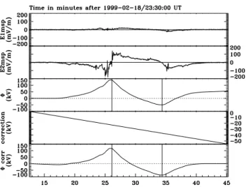
Fig. 1. First three panels show the two measured components of the electric field in the spin plane and the calculated potential along this dawn-to-dusk orbit above 40◦corrected geomagnetic latitude. The last two panels show the potential correction assuming a return to zero potential at low latitudes and the resulting corrected potential. The corotation electric field has been subtracted.
index, which reportedly is essentially the same as the asym-metric indices proposed by Clauer and McPherron (1980) and Clauer et al. (1983).
In this paper, we will examine the separate statistical re-sponses of polar cap convection and the field-aligned current system, which is believed to cause the low-latitude distur-bance to the solar wind. The large-scale convection and the geomagnetic disturbance are measured by the cross-polar po-tential drop, 8pc, and the ASY-H index, respectively.
2 Data
The Swedish Astrid-2 micro-satellite was launched on 10 December 1998 into an 83◦inclination polar orbit at 1000 km altitude and was spin-stabilized with a roughly Sun-pointing spin axis. In February and from mid-May until mid-June 1999, the satellite trajectory was in the dawn-dusk meridian plane and the probability of measuring most of the cross-polar potential drop 8pcwas then at its peak. An initial set of
101 two-cell convection events was singled out in the north-ern hemisphere throughout this period, assuming a symmet-ric noon-midnight two-cell convection pattern.
This assumption is incorrect, however. The interplanetary magnetic field (IMF) has a clear influence on the distribution of electric potential in the polar cap region. As the IMF By
goes from negative to positive for a given southward IMF, the location of the two potential extrema in the northern hemi-sphere rotates clockwise in magnetic local time (e.g. Shue and Weimer, 1994). Using the time shifted IMF and solar wind bulk velocity from the ACE spacecraft as input to the ionospheric convection model developed by Weimer (1996), we can produce a statistical convection pattern at the time of each Astrid-2 polar cap pass. The selection of events is
then optimized to where the satellite passes either through, or close to, both extrema of the Weimer model two-cell con-vection pattern. We further limit the data set to events where the IMF Bz <2 nT 15 min prior to each polar cap pass to
ensure the existence of a simple two-cell convection pattern. Figure 1 shows the electric field along the orbit of one of the 77 polar cap passes that remained after applying these criteria. The first two panels show the two components of the measured electric field in a model magnetic field B and spin plane coordinate system. The third component, E3msp,
along the Sun-pointing spin axis is not measured. E2mspis in
the spin plane, perpendicular to B and points in the dawn to dusk direction. E1mspcompletes the system. The corotation
electric field and the induced v × B electric field due to the motion of the satellite through the Earth’s magnetic field have both been subtracted from the measured field.
The electric potential 8 along the satellite trajectory is cal-culated by integrating the electric field above 40◦corrected
geomagnetic latitude (CGLat) for all passes, assuming that the spin axis electric field is zero. An example of the result-ing electric potential is shown in panel three of Fig. 1. The-oretically, 8 should return to zero potential at low latitudes due to the shielding effect of the plasmasphere (Shue and Weimer, 1994). The reason why there is usually a mismatch may be due to several contributing sources of error. First, we employ a model magnetic field instead of the measured field. Second, even though we find it reasonable to approximate the missing axial component of the electric field to be zero, due to the orientation of the orbital plane and the spin plane, it is, indeed, unknown. Finally, the measurement accuracy of the electric field on Astrid-2 is estimated to be approximately 3 to 5 mV/m. By adding a constant electric field of 3.8 mV/m, corresponding to the electric potential offset that is observed for the case shown in Fig. 1, we correct for the total effect of these errors and force the low latitude potential back to zero (see the last two panels in Fig. 1).
The potential drop 8pcis essentially a time averaged
quan-tity, since it is acquired over the time in between the two large-scale convection reversals (marked by vertical bars in Fig. 1). We, therefore, average the 1-min resolution ASY-H index over the same time interval, which is identified by its middle time, tm, so that both quantities are comparable in
time.
The time it takes for the solar wind to propagate from the ACE spacecraft, at the L1-point, to an average magnetopause location of 11 RE(Fairfield, 1971), is computed individually
for each measurement of 8pcby taking the mean of the solar
wind bulk velocity two hours prior to tm, and applying both
the xgseand ygsevelocity components (Eriksson et al., 2000).
As a consequence of the finite Pedersen conductivity in the high-latitude ionosphere, we expect the large-scale convec-tion electric field to gradually respond after some addiconvec-tional time delay following the arrival of a solar wind structure at the magnetopause (e.g. Sanchez et al., 1991). The time of zero magnetospheric time lag is defined here by subtracting only the propagation time from tmfor each event.
Fig. 2. The time shifted IMF Bzand reconnection electric field Er
measured at the ACE spacecraft are plotted versus time lag 1t . A negative time lag refers to future solar wind conditions. Note the different vertical ranges on the y-axes.
the two sets of 8pc and ASY-H to the driving solar wind, we
will study how their correlation coefficients with two solar wind quantities evolve as a function of time lag.
3 Magnetospheric response to the solar wind
The applied solar wind quantities, both in GSM coordinates, are the IMF Bz and the model reconnection electric field
Er =vBtsin4(θ/2), respectively. Here, v is the solar wind
bulk velocity in xgsm direction, Bt is the projection of the
IMF onto the GSM y − z plane, and θ is the clock angle be-tween Bt and the positive zgsmdirection. These solar wind
parameters have been shown to correlate well with the cross-polar potential drop (Reiff and Luhmann, 1986; Eriksson et al., 2000, and references therein).
Figure 2 shows the time shifted IMF Bzand Erversus time
lag 1t for two cases plotted next to each other. The mea-sured potential drop along the orbit and the average ASY-H are indicated explicitly for both events, as well as the propa-gation time and the mid-time tm. We observe that the
poten-tial drop and the low-latitude asymmetric geomagnetic dis-turbance are, indeed, larger for a correspondingly larger IMF
Bzand electric field, as expected.
We now proceed to calculate a correlation coefficient be-tween the set of 77 cross-polar potential drops and the two corresponding sets of solar wind parameters at 1t=0. For each new 5-min resolution time lag in the range −10 to 150 min, we calculate a new correlation coefficient as the solar wind parameters are changed (see Fig. 2 for the solar wind input as a function of time lag for two of the 77 events). The resulting correlation coefficients for both 8pc and
ASY-H with the solar wind as a function of time lag is illustrated in Fig. 3a-b. The maximum correlation coefficient r and its corresponding time lag 1t are shown for each combination of magnetospheric parameter and solar wind quantity.
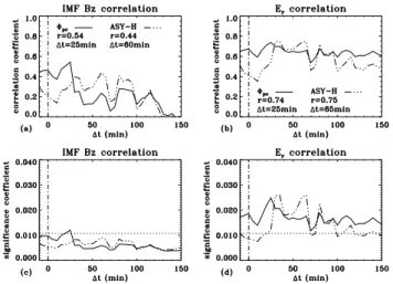
Fig. 3. Solar wind-magnetosphere correlation with (a) IMF Bz, and
(b) reconnection electric field. The corresponding filtered correla-tion coefficients are shown in (c) and (d), where the horizontal line marks r = 0.50. Time resolution is 5 min. The maximum correla-tion coefficients and corresponding time lag 1t are shown on each panel.
Since we are more interested in correlation coefficients above r = 0.50 than below, we filter the correlation coef-ficients through y(r) = a tan(r + c), where a = 1/200.071 and c = 0.6349 are two constants found by a minimum least squares functional fit of the data in Eriksson et al. (2000). The filter is based on a bootstrap technique (Efron and Tib-shirani, 1993) for the derivation of a correlation coefficient standard error, which is used to quantify the bootstrap dis-tribution produced for each correlation coefficient. This fil-ter was recently developed by Eriksson et al. (2000). The resulting non-normalized filtered correlation coefficients y, here referred to as significance coefficients, are shown in Fig. 3c-d. The lower horizontal dotted line marks the level of
r =0.50. We see that the 8pc response to the reconnection
electric field peaks at 1t = 25 min after which it slowly decays, whereas ASY-H first responds after about 35 min, then at 65 min, and finally shows an increased response at
1t =80 min. The first two peaks have a correlation coeffi-cient r = 0.75, while the last peak has r = 0.72.
4 Results and discussion
It has been shown in previous studies that 8pcgenerally
cor-relates better with parameters including both the solar wind velocity and the IMF Bz, than with IMF Bzalone (e.g. Baker
et al., 1983; Reiff and Luhmann, 1986; Eriksson et al., 2000). This is again evident in comparing the correlation coeffi-cients for IMF Bzand Er with 8pcin Fig. 3a-b.
The data and time lags for which the correlation is max-imized between 8pc and the two solar wind quantities are
shown in Fig. 4a-b along with an expression for its best lin-ear fit (solid line). The corresponding linlin-ear fits (dashed line) from a recent study using the FAST satellite and the Wind
652 S. Eriksson et al.: Magnetospheric response to the solar wind
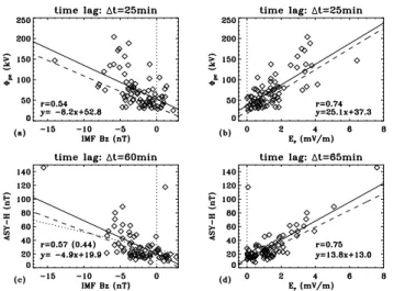
Fig. 4. Cross-polar potential drop versus (a) IMF Bz, and (b) Erat
the time lag of peak correlation. ASY-H versus (c) IMF Bzand (d)
Er, also for optimum time lag. Best linear fit for Astrid-2 and ACE
spacecraft (solid line), and for FAST and Wind spacecraft (dashed line).
spacecraft (Eriksson et al., 2000) that comprised 37 events, are shown as well, and we see that the slopes are in good agreement. The optimized time lags for 8pc in the FAST
study were found to be 15 min for both IMF Bzand Er. This
response peak was interpreted as the direct or driven magne-tospheric response to the solar wind input and confirmed the line-tying time scale previously reported (Lockwood et al., 1990; Sanchez et al., 1991). The 8pc response to Er was
followed by two minor peaks at time lags 1t =55 min and
1t=105 min. These secondary pulses were both interpreted as unloading responses of the magnetotail.
Here, the maximum response for 8pc is approximately
25 min. The difference in time lag between the two stud-ies is most likely due to the different positions of the two solar wind upstream monitors. Wind was located closer than 90 RE upstream of the Earth, whereas ACE was positioned
around 240 RE. This separation increases the uncertainty in
the calculation of correct propagation times. It should also be noted that the time lags represent the total delay for the large-scale convection to respond to changes at the assumed average magnetopause position of 11 RE.
Using the average ASY-H magnetic index instead of 8pc
in the correlation with the solar wind, results in the linear best fits displayed in Fig. 4c-d for the time lags of peak correlation. Performing a linear regression analysis for the ASY-H response to Er at 1t =35 min gives the expression
y(x) =15.8x + 10.8. The third peak at 1t =80 min results in y(x) = 11.9x + 15.4. As the delay time increases, the best fit slope is observed to gradually decrease. This implies that on the average, the shorter the delay is, the larger the depression for a constant reconnection electric field at the magnetopause. An underlying assumption is that ASY-H at any one time reflects the superposition of contributions from direct input responses as well as delayed geomagnetic tail
responses.
In comparing Fig. 4b with Fig. 4d we note that there is a larger scatter for the 8pcdata than for ASY-H, which may be
attributed to the effect of not measuring the complete cross-polar potential drop. The solid line in Fig. 4c only uses the 73 points shown, while the dotted line also includes the four points with IMF Bz>3 nT.
The two studies are clearly different for both the ASY-H response and the 8pc response. For the FAST study, with
data from July 1997, the geomagnetic activity was lower than
Kp =4−and the major response of ASY-H to Er peaked
be-tween 60 and 75 min. Here, with a maximum Kp = 7−, we mainly observe a twin peak with an initial fast response at
1t=35 min and a second peak at 65 min time lag. This dif-ference may be due to the effect of examining the magneto-spheric response for different levels of geomagnetic activity. The largest potential drop included in this data set, 8pc=204
kV (see Fig. 1 for the electric field), was measured approxi-mately 10 hours after the magnetic storm on 18 February had reached a minimum Dst = −134 nT. Moreover, this data set contains a total of 21 events when the geomagnetic activity level was greater than Kp = 4−.
Bargatze et al. (1985) reported on two major pulses at about a 20 and 60 min time lag in their study of the westward electrojet AL index response to the solar wind input vBs for
different levels of geomagnetic activity. As the level of ge-omagnetic activity increased from moderate to strong, they discovered that the directly driven 20 min response started to dominate over the 60 min unloading response. Both pulses were present for moderate activities, but the 60 min response was more pronounced. In this study of higher geomagnetic activity, the 8pc response to Er has a broad single peak
around 25 min lag, whereas ASY-H responded to Er with
three multiple peaks of 35, 65, and 80 min lags. In an ear-lier study, using FAST data for a lower level of geomagnetic activity, a mirror image was found. The 8pcthen responded
to Er with three multiple peaks, whereas ASY-H responded
with one broad peak around a 60–75 min lag. We believe these differences may be attributed to different levels of ge-omagnetic activity and to differences in the overall geophys-ical conditions for the different events. This follows from studying the AL response to vBs for different geomagnetic
activities, as shown in Fig. 3 of Bargatze et al. (1985). By going from their filter 21 to filter 14 say (i.e. from higher activity to lower activity), we observe two peaks at approx-imately 20 min and 55 min in filter 21, but only one broad peak around 60 to 70 min of filter 14. This trend is observed for the ASY-H response to Ergoing from the Astrid-2 results
to the FAST results (Eriksson et al., 2000). A similar trend is observed for 8pcto Er, going from filter 27 of higher
activ-ity, showing a single broad peak around 20 min, to filter 21 of lower activity.
The auroral electrojets have been reported to respond only on the shorter 20 min time scale for periods of enhanced ge-omagnetic activity (Baker et al., 1983). This may explain the lack of clear secondary unloading responses to the reconnec-tion electric field for 8pc, which was observed, however, to
occur in the FAST study for a lower level of geomagnetic activity.
The ASY-H response to the reconnection electric field ex-amined here is further quantitatively consistent with the re-sults obtained by Clauer and McPherron (1980), in which they report that large low-latitude asymmetric disturbances (> 25 nT) were consistently preceeded by an enhanced dawn-dusk solar wind electric field for a total of 24 events.
To summarize, we have examined the average time de-layed response of the ionospheric convection and the low-latitude horizontal geomagnetic disturbance to the 5-min res-olution reconnection electric field for a total of 77 events. We find that it is possible to observe the directly driven response of the high-latitude convection around 25 min, and the de-layed unloading response of the field-aligned current sys-tem primarily around 65 min, as measured by ASY-H. These individual responses were also identified by Eriksson et al. (2000) for a lower geomagnetic activity level. We further suggest that the high level of geomagnetic activity recorded in this study increases the efficiency for the solar wind to di-rectly drive the region 1 and region 2 field-aligned current systems, which are believed to be a major cause for the low-latitude asymmetric depression in the horizontal component of the geomagnetic field (Crooker and Siscoe, 1981). This earlier ASY-H response is estimated to be delayed by 35 min after the solar wind has reached the magnetopause, which is somewhat longer than for the convection to respond. This may support the idea proposed by Clauer et al. (1983) that the reconnection electric field primarily drives the ionospheric convection and that the global Birkeland current system, in turn, must respond to changes in the convection. However, it is the purpose of a future study to verify the possible internal delays between the ionospheric convection and the westward electrojet, since in the study of Bargatze et al. (1985), only
ALwas used and 8pcwas omitted.
Acknowledgement. We would like to thank the ACE team, and
es-pecially Dr. Andrew Davis at Caltech, and Dr. Ruth Skoug at LANL, for providing the solar wind data. We also thank Dr. T. Iyemori and the World Data Center at Kyoto in Japan for the ge-omagnetic activity data, and Dr. John Bonnell at Space Sciences Laboratory, University of California at Berkeley for valuable com-ments and discussions.
Topical Editor G. Chanteur thanks R. Clauer and another referee for their help in evaluating this paper.
References
Baker, D. N., Zwickl, R. D., Bame, S. J., Hones, E. W. Jr., Tsurutani, B. T., Smith, E. J., and Akasofu, S.-I., An ISEE 3 high time res-olution study of interplanetary parameter correlations with mag-netospheric activity, J. Geophys. Res., 88, 6230–6242, 1983. Bargatze, L. F., Baker, D. N., McPherron, R. L., and Hones, E.
W. Jr., Magnetospheric impulse response for many levels of geo-magnetic activity, J. Geophys. Res., 90, 6387–6394, 1985. Blanchard, G. T. and McPherron, R. L., Analysis of the linear
response function relating AL to VBs, J. Geophys. Res., 100,
19155–19165, 1995.
Clauer, C. R. and McPherron, R. L., The relative importance of the interplanetary electric field and magnetospheric substorms on partial ring current development, J. Geophys. Res., 85, 6747– 6759, 1980.
Clauer, C. R., McPherron, R. L., and Searls, C., Solar wind con-trol of the low-latitude asymmetric magnetic disturbance field, J. Geophys. Res., 88, 2123–2130, 1983.
Crooker, N. U. and Siscoe, G. L., Birkeland currents as the cause of the low-latitude asymmetric disturbance field, J. Geophys. Res., 86, 11201–11210, 1981.
Efron, B. and Tibshirani, R. J., An Introduction to the Bootstrap, Mono. Stat. Appl. Prob., 57, 436 pp., Chapman and Hall, New York, 1993.
Eriksson, S., Ergun, R. E., Carlson, C. W., and Peria, W., The cross-polar potential drop and its correlation to the solar wind, J. Geo-phys. Res., 105, 18639–18653, 2000.
Etemadi, A., Cowley, S. W. H., Lockwood, M., Bromage, B. J. I., Willis, D. M., and Luhr, H., The dependence of high-latitude ionospheric flows on the north-south component of the IMF: A high time resolution correlation analysis using EISCAT Polar and AMPTE UKS and IRM data, Planet. Space Sci., 36, 471–498, 1988.
Fairfield, D. H., Average and unusual locations of the Earth’s mag-netopause and bow shock, J. Geophys. Res., 76, 6700–6716, 1971.
Fukushima, N. and Kamide, Y., Partial ring current models for worldwide geomagnetic disturbances, Rev. Geophys. Space Phys., 11, 795–853, 1973.
Harel, M., Wolf, R. A., Reiff, P. H., Spiro, R. W., Burke, W. J., Rich, F. J., and Smiddy, M., Quantitative simulation of a mag-netospheric substorm, 1, Model logic and overview, J. Geophys. Res., 86, 2217–2241, 1981.
Holzer, T. E. and Reid, G. C., The response of the dayside magnetospheionosphere system to time-varying field line re-connection at the magnetopause, I, Theoretical model, J. Geo-phys. Res., 80, 2041–2049, 1975.
Iyemori, T., Maeda, H., and Kamei, T., Impulse response of geo-magnetic indices to interplanetary geo-magnetic field, J. Geomagn. Geoelectr., 31, 1–9, 1979.
Iyemori, T. and Rao, D. R. K., Decay of the Dst field of geo-magnetic disturbance after substorm onset and its implication to storm-substorm relation, Ann. Geophysicae, 14, 608–618, 1996. Lockwood, M., Cowley, S. W. H., and Freeman, M. P., The exci-tation of plasma convection in the high-latitude ionosphere, J. Geophys. Res., 95, 7961–7972, 1990.
Reiff, P. H. and Luhmann, J. G., Solar wind control of the polar-cap voltage, in: Solar Wind-Magnetosphere Coupling, Eds. Y. Kamide and J. A. Slavin, pp. 453–476, Terra Sci., Tokyo, 1986. Sanchez, E. R., Siscoe, G. L., and Meng, C.-I., Inductive attenuation
of the transpolar voltage, Geophys. Res. Lett., 18, 1173–1176, 1991.
Shue, J.-H. and Weimer, D. R., The relationship between iono-spheric convection and magnetic activity, J. Geophys. Res., 99, 401–415, 1994.
Todd, H., Cowley, S. W. H., Etemadi, A., Bromage, B. J. I., Lock-wood, M., Willis, D. M., and Luhr, H., Response-time of the high-latitude ionosphere to sudden changes in the north-south component of the IMF, Planet. Space Sci., 36, 1415–1428, 1988. Weimer, D. R., A flexible, IMF-dependent model of high-latitude electric potentials having “space weather” applications, Geo-phys. Res. Lett., 23, 2549–2552, 1996.