On the Interest of Bulk Conductivity Measurements for Hydraulic Dispersivity Estimation from Miscible Displacement Experiments in Rock Samples

HAL Id: hal-01372008

https://hal.sorbonne-universite.fr/hal-01372008

HAL is a multi-disciplinary open access archive for the deposit and dissemination of sci-entific research documents, whether they are pub-lished or not. The documents may come from teaching and research institutions in France or abroad, or from public or private research centers.

L’archive ouverte pluridisciplinaire HAL, est destinée au dépôt et à la diffusion de documents scientifiques de niveau recherche, publiés ou non, émanant des établissements d’enseignement et de recherche français ou étrangers, des laboratoires publics ou privés.

On the Interest of Bulk Conductivity Measurements for

Hydraulic Dispersivity Estimation from Miscible

Displacement Experiments in Rock Samples

Alexis Maineult, Jean-Baptiste Clavaud, Maria Zamora

To cite this version:

Alexis Maineult, Jean-Baptiste Clavaud, Maria Zamora. On the Interest of Bulk Conductivity Mea-surements for Hydraulic Dispersivity Estimation from Miscible Displacement Experiments in Rock Samples. Transport in Porous Media, Springer Verlag, 2016, 115 (1), pp.21-34. �10.1007/s11242-016-0749-0�. �hal-01372008�

TECHNICAL NOTE

1

2

On the interest of bulk conductivity measurements for hydraulic dispersivity estimation

3

from miscible displacement experiments in rock samples.

4

5

Alexis Maineult 1,2,+, Jean-Baptiste Clavaud 1,* and Maria Zamora 1 6

7

1) Institut de Physique du Globe de Paris, Sorbonne Paris Cité, Univ Paris Diderot, UMR 7154 8

CNRS, 1 rue Jussieu, 75005 Paris, France 9

2) Sorbonne Universités, UPMC Univ Paris 06, CNRS, EPHE, UMR 7619 Metis, 4 place 10

Jussieu, 75005 Paris, France 11

* _{now at Chevron Energy Technology Company, 1500 Louisiana St., Houston, TX 77002, USA}

12

13

14

+ _{corresponding author. Phone: +33 (0)1 44 27 43 36. E-mail address: alexis.maineult@upmc.fr}

15

SUMMARY

17

The determination of the hydraulic dispersivity and effective fraction of porous medium 18

contributing to transport on soil and rock sample in the laboratory is important to understand and 19

model the evolution of miscible contaminant plumes in groundwater. Classical methods are based 20

on the interpretation of the breakthrough curve, i.e., the evolution of the concentration in 21

contaminant at the downstream end-face of a sample into which a front of contaminant is 22

advected. Here we present an experimental device aimed at performing such measurements, but 23

also allowing the bulk electrical conductivity of the sample to be measured. We show that the 24

dispersivity and effective fraction can be inferred from this electrical measurement, and that the 25

combined use of both out-flowing fluid conductivity and bulk conductivity allows the incertitude 26

on the dispersivity and effective fraction to be significantly enhanced. 27

28

Keywords: miscible displacement, hydraulic dispersivity, breakthrough curve, electrical

29

conductivity 30

1. Introduction

32

33

Miscible contaminants flowing through a porous medium by advection are mixing with 34

the non-contaminated water, yielding to dilution of the plume. This so-called dispersion 35

phenomenon originates from the fact that the fluid moves faster in larger pores than in smaller 36

ones and faster in the centres of the pores than along the walls, and also that some pathways are 37

longer than others (e.g., Fetter 2001). If we consider an isotropic and homogeneous soil or rock 38

sample, and assume that i) the flow through it is purely one-dimensional and ii) the dispersion 39

process is Fickian, the concentration field C(x,t) (in mol m–3) inside the sample, where x (in m) 40

stands for the distance from the upstream-face of the sample and t (in s) for the elapsed time, 41

obeys the transport equation: 42 2 2 C C C D v t x x ∂ ₌ ∂ ₋ ∂ ∂ ∂ ∂ , (1) 43

Here D is the hydrodynamic dispersion coefficient (in m2 s–1) and v the linear average velocity of 44

water flowing through the sample (in m s–1). Provided that diffusion processes can be neglected, 45

the dispersion coefficient in Eq. (1) can be written D = λv, where λ is the hydraulic dispersivity 46

(in m). Even though the dispersivity changes with the observation scale (e.g., Xu and Epstein 47

1995), it is often required to determine its value on soil or rock samples to understand and model 48

the dynamics of contaminants at the field scale. 49

The classical way to perform such measurements in the laboratory consists in applying a 50

straight front of salty solution at the entrance (i.e., the upstream face) of the sample subjected to 51

permanent, laminar flow, and to measure the concentration at the outlet (i.e., the downstream 52

face). The evolution of the concentration of the out-flowing fluid, or “breakthrough curve”, is 53

generally sigmoidal, provided that the medium is homogeneous at the scale of the sample and 54

that no other processes occur, such as chemical reactions with the minerals. The spreading of the 55

curve increases with the dispersivity. Knowing the theoretical formulation of the breakthrough 56

curve, it is then possible to determine the value of the dispersivity by fitting methods. 57

The out-flowing concentration is an integrated value, which presents variations only when 58

the salt front reaches the downstream face of the sample. Other methods, such as electrical 59

measurements, can give information as soon as the salt front penetrates the sample. For example, 60

Odling et al. (2007) used electrical impedance measurements on microfractured granite to 61

determine its longitudinal dispersivity. They showed that such a technique provided supplemental 62

information about the dispersion process inside the sample. Here we report on an apparatus 63

allowing the bulk conductivity of a rock sample to be measured during miscible displacement 64

experiments. We show that fitting the classical breakthrough curve to the measured electrical 65

conductivity of the out-flowing fluid, combined to fitting the theoretical evolution of the bulk 66

conductivity of the sample to the measured one, enables a more accurate determination of the 67

hydraulic dispersivity and fraction of the porous volume effectively contributing to the transport. 68

69

2. Materials and method

70

71

2.1. Device and procedure

72

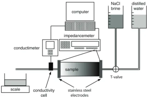
We devised, constructed and tested an experimental set-up (Fig. 1), aimed at measuring 73

the bulk electrical conductivity σb (in S m–1) of large-sized samples (i.e., about 5 to 10 cm in

74

diameter and 10-40 cm or more in length), as well as the electrical conductivity of the fluid that is 75

out-flowing from the sample, denoted σf. This device is usable to perform miscible displacement

76

experiments and therefore infer the hydraulic dispersivity λ (in m) and the effective fraction of 77

the porous volume contributing to transport, denoted f (no unit). 78

The upstream and downstream end-faces of the sample, which is placed horizontally to 79

avoid the influence of gravity, are connected to a hydraulic circuit. They are also in perfect 80

contact with stainless steel electrodes, whose external side is protected by a PVC cap to ensure 81

electrical isolation. The conductivity of the out-flowing fluid is measured with a custom-made 82

cell with four platinum electrodes that was calibrated with various brines at different frequencies. 83

The fluid conductivity and the bulk conductivity of the sample are measured with an impedance-84

meter HP 4263A, at the frequencies of 120 and 1000 Hz. The optimal frequency, which 85

minimizes the polarization effects, is equal to 1 kHz. Note that concerning the bulk conductivity, 86

the measure is done with the two electrodes at the end-faces of the sample only, each electrode 87

serving for both current injection and potential measurement. 88

To check its watertightness, the sample is first put under vacuum for a few hours. The 89

sample is then saturated with distilled and de-aerated water. The porosity accessible by water 90

under vacuum, which is close to the connected porosity, is deduced from the amount of injected 91

water required to fill the connected voids, with an accuracy comprised between 0.3 and 3.5 92

percents. Then we let the fluid flowing through the sample from the upstream reservoir filled 93

with distilled water. Once the chemical equilibrium is reached, i.e. when the conductivity of the 94

out-flowing fluid is constant, the distilled water saturating the sample is flushed by NaCl brine at 95

a concentration around 3 g L–1, coming from the brine reservoir. This value of the concentration 96

is large enough to consider the contribution of the surface conduction to the total electrical 97

conductivity negligible, but small enough to neglect density-driven flow, at least for highly 98

permeable samples. Brine is injected until the out-flowing solution has the same electrical 99

conductivity. In practice, a given amount of brine is introduced in the sample. The electrical 100

measurements are carried out rapidly enough to neglect the effects of pure diffusion and reduce 101

the density effects, if any. Afterwards we proceed to a new injection step, and so on. 102

103

2.2 Tested sample

104

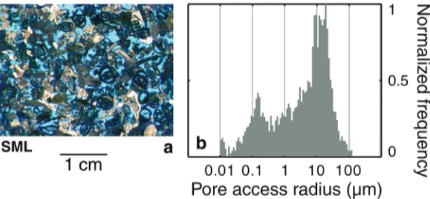
To test our approach, we use a decimetric core of Saint-Maximin limestone (denoted 105

SML). It is a bioclastic limestone, having a large macro-porosity, and a small amount of 106

intraclastic porosity (Fig. 2a). The results of mercury injection carried out on a centimetric core 107

(Fig. 2b) show that the distribution of the pore access radii is bi-modal with to modes at 13.6 and 108

0.13 µm respectively. However, the second mode, which corresponds to the intraclastic porosity, 109

is clearly dominated by the first mode. 110

The sample was 309 mm in length, with a diameter of 97.90 mm. The volume of the 111

sample (2326 cm3) is therefore two orders of magnitude larger than the volumes of rock samples 112

commonly studied in the laboratory for permeability estimation (i.e., 20 to 50 cm3). This size was 113

chosen to acquire measurements at a scale significantly larger than the representative elementary 114

volume (e.g., Henriette et al. 1989). After machining, the sample was dried in an oven at 60 °C 115

for several days, until its weight stabilized. Then the lateral surface was waterproofed by 116

covering it with epoxy resin. The connected porosity value, determined from weighting, was 117

equal to 36.6 ± 0.5 %. From flow-rate measurement, the water permeability was estimated to be 118

1718 ± 42 mD. 119

To check if advection is predominant over diffusion in our experiment, we estimated the 120

Péclet number Pe. The classical formulation Pe = vDF d / Dm (e.g., Sahimi 1993), where vDF is the

121

Dupuit-Forcheimer velocity (in m s–1), d the mean grain diameter (in m) and Dm the molecular

122

diffusion coefficient (1.5 10–9 m2 s–1 for NaCl), is not applicable for non-granular rocks. 123

Therefore, we used the non-correlation radius rnc, estimated from image analysis, instead of d/2.

This yields to Pe = 2 vDF rnc / Dm. For the highly permeable sample SML, vDF was equal to 0.35

125

mm s–1 during the experiment, and rnc was estimated to 175 µm. The Péclet number is thus

126

around 80, meaning that in this case advection can be neglected (power-law regime, e.g. Sahimi 127

1993). 128

For the miscible displacement experiment, the conductivity of the initial fluid after 129

stabilization was equal to 4.7 mS m–1. The conductivity of the injected fluid was 540 mS m–1. 130

(i.e., 54.3 mmol L–1 or 3.17 g L–1 NaCl). The bulk conductivity of the sample was equal to 1.4 131

mS m–1 initially, and to 90.1 mS m–1 at the end of the experiment, yielding to an electrical 132

formation factor F = σf / σb equal to 6.

133

134

3. Theory

135

136

3.1. Problem and solution for a 1D isotropic and homogeneous medium

137

Considering that Eq. (1) applies to our case, the initial condition is C(x,0) = C0, where C0

138

is the equivalent salt concentration of the solution initially saturating the pore space. The 139

upstream boundary condition, corresponding to the injection of brine starting at t = 0, can be 140

formalized as C(0,t) = C0 + (Cbrine – C0) H(t) where Cbrine is the concentration of the brine and H

141

the Heaviside step function. The solution is given by (e.g., Ogata and Banks 1961; Fried and 142

Combarnous 1971; Gupta and Greenkorn 1974; Basak and Murty 1979): 143

( )

0

, erfc exp erfc

2 2 2 C C x vt vx x vt C x t C D Dt Dt   −  −     +  = + _{  }+ _{    }      , (2) 144

where erfc is the complementary error function. The second term in the brackets has an influence 145

only if t is close to 0, and can be neglected otherwise (e.g., Ogata and Banks 1961; Pfannkuch 146

1963), yielding to the following approximation of Eq. (2): 147

( )

3.2. Non-dimensionalization of the solution

150

In order to compare the breakthrough curves for different samples, if any, it is convenient 151

to use the normalized variation of the concentration δC (no unit) defined by 152

( )

( )

Since the injection is not continuous but performed step by step (see end of section 2.1), it is 154

convenient to consider δC as a function of the normalized injected volume of brine Vin, expressed

155

in pore volumes, as (e.g., Pickens and Grisak 1981): 156 n i i pc V V V = , (5) 157

where Vi is the injected volume of brine and Vpc the total connected porous volume of the sample,

158

equal to the total porosity times the volume of the sample. Following this way, the curves δC 159

versus Vin for different samples are similarly scaled and therefore directly comparable. Indeed,

160

the time required for the injection of a given volume of brine, which depends on the permeability 161

of the rock, is eliminated from Eq. (3): considering that Vin is also equal to v t / L where L is the

162

length of the sample (in m), and assuming that the molecular diffusion is negligible so that we 163

can introduce the hydraulic dispersivity as λ = D / v, the combination of Eqs. (3) and (4) leads to: 164

( )

The normalized variation of concentration of the out-flowing solution, denoted δCout, is obtained

by taking x = L in Eq. (6): 167

( )

( )

Classically, the λ / L ratio is inferred from the measured values of δCout (i.e., the normalized

169

breakthrough curve) by fitting the theoretical curve (Eq. (7)) to them. Note here that this 170

theoretical curve passes through the point M1,0.5 = (Vin,δCout) = (1,0.5), since the volume of brine

171

required for the centre of mass of the front to arrive at the downstream end of the sample is equal 172

to one pore volume. 173

It is assumed here that the whole connected pore volume contributes to the transport, but 174

it is rarely expected. For example, dead-end pores do not contribute to the transport processes. If 175

the pore volume contributing to transport (or “efficient porosity”), denoted Vpc*, is smaller than

176

Vpc, the experimental curve δCout versus Vin is shifted to the left. In other words, the injected

177

volume, normalized using Eq. (5), for which δCout is equal to 0.5, is smaller than 1. In this case,

178

one should also find the best Vpc* to be used in place of Vpc in Eq. (5). To do so, we define the

179

effective fraction of the porous volume contributing to the transport as f = Vpc*/Vpc. Equation (5)

180

must thus be rewritten as: 181 * n i i i pc pc V V V V fV = = . (8) 182

The problem then involves two parameters, λ/L and f, to be found using Eqs. (7) and (8). 183

It should be noted here that if no theoretical curve can explain the data, it means that the 184

medium is not homogeneous, and/or that retardation processes occur such as trapping in small 185

pores, or that molecular diffusion is not negligible, or that density-driven flow occurs, or even 186

chemical reactions with the reactive mineral phases happen. 187

Finally, note that for the calculation of Vin, the measured injected volume of brine was

188

corrected from the volume of the tube between the T-valve (Fig. 1) and the upstream end of the 189

sample for the bulk sample conductivity, and from the same volume plus the volume of the tube 190

between the downstream end of the sample and the conductivity cell for the conductivity of the 191

out-flowing fluid. 192

193

3.3. Conversion of conductivity to concentration

194

As previously stated, we do not measure the salt concentration directly, but the electrical 195

conductivity of the fluid. To transform the concentration C into conductivity σf, and reciprocally

196

σf into C, we use the empirical relations established by Sen and Goode (1992) for NaCl brine:

197

(

)

where T is the temperature (in °C) and M is the molality (in mol kg–1). To convert the 199

concentration Cf into molality, we use the CRC Handbook Table at 20°C (Lide 2008).

200

For coherence, we also normalized the conductivity of the out-flowing fluid, σout, as:

201

( )

( )

where σout,0 and σout,max are the initial and maximal (i.e., the plateau value at the end of the

203

experiment) conductivities of the effluent solution, respectively. We proceeded similarly for the 204

bulk conductivity of the sample σb:

205

( )

( )

where σb,0 is the initial and σb,max the maximal (i.e., the plateau value at the end of the

207

experiment) value of the bulk conductivity. 208

209

4. Estimation of the dispersivity

210

To estimate the dispersivity λ, we first use the classical method, which consists in fitting a 211

straight line in Henry’s space to the experimental points of the out-flowing fluid concentration. 212

Secondly we systematically explored the parameter space. This second method allows the 213

effective fraction f to be taken into account, and the sample conductivity to be also considered. 214

215

4.1. Cost-function

216

To evaluate the agreement between the data (i.e., the normalized measured conductivity 217

variations) and the model (i.e., the normalized predicted conductivity variations), a cost-function 218

R as meaningful as possible has to be defined. We used the determination coefficient r2, which 219

quantifies the mean deviation of the N experimental points (vector dobs) from the predictions 220 (vector dpred): 221

(

)

(

)

∑

∑

Moreover, considering that the concentration break-through curves (Eq. (7)) are similar to 223

cumulative Gaussian distributions, we combined r2 with the Kolmogorov-Smirnov (KS) test (e.g., 224

Press et al. 1997), usually used as an estimator of the semblance between two distributions, given 225 by: 226

( )

∑

We thus used the function R = KS r2; an optimal fit is obtained when R = 1. 228

229

4.2. Fitting method in Henry’s space

230

Defining the two parameters α (no unit) and Γ (no unit) as: 231 1 2 1 n i n i L V V α λ  =    ₋ Γ =  , (14) 232

Eq. (7) can be rewritten as: 233

( )

( )

Therefore the curve Γ versus δCout plotted in linear arithmetic probability paper (in ordinates)

235

forms a straight line (e.g., Brigham 1974), also called Henry’s line. The slope of this line, 236

denoted p, is theoretically given by: 237 1 2 2 p L λ α = − = − . (16) 238

We did not apply the classical two-point Taylor’s (1953) method to determine λ (e.g., Fried and 239

Combarnous 1971; Gupta and Greenkorn 1974; Pickens and Grisak 1981). Instead, we 240

determined the straight line fitting the data in the least-square sense, as suggested by Gupta and 241

Greenkorn (1974), considering that this method provides more accurate values for the slope p. 242

Note that in this case it is necessary to restrict the data to the interval for which the conductivity 243

variation is linear, i.e., generally for δCout comprised between 0.1 and 0.9. The dispersivity is then

244

deduced using Eq. (16) as λ = L p2 / 2. 245

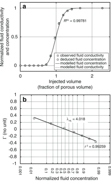
The observed normalized conductivity δσout and deduced normalized concentration δCout

246

of the out-flowing fluid as a function of the volume of injected brine Vin, expressed in fraction of

porous volume, are shown in Fig. 3a for SML sample. The concentrations δCout are distributed

248

along a sigmoid, which seems to pass very close to the point M1,0.5 = (Vin,δCout) = (1,0.5),

249

meaning that the whole pore volume contribute to the transport. The associated Γ values 250

computed using Eq. (14), versus normalized experimental concentration δCout, are distributed

251

along a straight line (Fig. 3b). The line fitting the best the data, in the least-squares sense, passes 252

through the point (δCout,Γ) = (0.5,0), meaning that indeed the effective fraction f is equal to 1.

253

The slope of the fitting line gives a value of 4.018 mm for the dispersivity λHL. The modelled

254

curves δCout (continuous line in Fig. 3a, obtained with Eqs. (7) and (5)) and δσout (dotted line)

255

versus the volume of injected brine, expressed in fraction of porous volume, explain the data 256

rather well (the cost-function RHL _{is close to 1.0).}

257

258

4.3. Parameter space exploration

259

The previous procedure takes into account the conductivity variation of the out-flowing 260

fluid only. Moreover, it does not provide a confidence interval for the dispersivity or the effective 261

fraction of porous volume. We hereafter estimate the dispersivity directly from the curves of the 262

out-flowing fluid conductivity variations δσout or/and the variations of the bulk conductivity δσb

263

versus the injected volume Vin by exploring the parameter space

264

To estimate the sample bulk conductivity σb, we apply the generalized Reuss average,

265

since the measurement is performed in the direction of the concentration gradient. We assume 266

that i) the concentration front is one-dimensional along the axis of the sample (i.e., the sample is 267

homogeneous and the front is straight, i.e., the density effect are negligible), and ii) the formation 268

factor F does not depend on the value of the local fluid conductivity. Therefore, σb can be written

269

as (Odling et al. 2007): 270

( )

(

( )

)

∫

where σf (C(x,t)) corresponds to the fluid conductivity distribution inside the sample (computed

272

using Eqs. (3) and (9)). It is important to note that the knowledge of the formation factor is not 273

required, since it vanishes in the computation of the normalized variation of the bulk conductivity 274

using Eq. (11). 275

The application to limestone SML is shown in Figs. 4, 5 and 6. We explored the 276

dispersivity values in the interval comprised between 0 and 20 mm (based on the value 277

previously determined for λHL,) with a spacing of 0.1 mm, and the values of the effective fraction

278

in the interval comprised between 0.85 and 1 with a spacing of 0.001. 279

When the exploration method is applied to the fluid conductivity only (Fig. 4a), the 280

maximal value of the cost-function Rfmax is equal to 0.99951 (with a Kolmogorov-Smirnov value

281

equal to 100 %) and corresponds to a dispersivity λf (subscript "f" standing for "fluid") of 4.0 mm

282

and an effective fraction ff of 0.982. The value of the dispersivity is very close to the value

283

determined previously using Henry’s line (4.018 mm). The value of the effective fraction is very 284

close to 1, but is slightly smaller. The predictions computed with Eqs. (7), (8) and (10) explain 285

very well the data (Fig. 4b). 286

We proceeded similarly for the bulk conductivity only (Fig. 5). As for the fluid, the 287

normalized bulk conductivity of the sample is sigmoidal, but the bulk conductivity evolves as 288

soon as brine is injected in the sample (Fig. 5b). The dispersivity λs (subscript "s" standing for

289

"sample") is equal to 3.3 mm, a value slightly smaller than λf. The effective fraction fs is equal to

290

0.987. The prediction, computed using Eqs. (3), (9), (11) and (17), explains here again rather well 291

the data, with a cost-function Rsmax equal to 0.99954. However, it seems that the dispersivity may

be slightly underestimated for injected volume above 1, the prediction being systematically 293

higher than the experimental points. 294

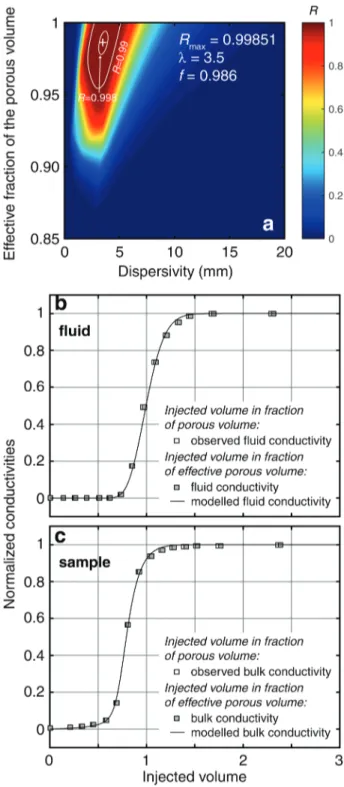
We finally apply the same methodology to find the best dispersivity and effective fraction 295

explaining both fluid and sample conductivities simultaneously (Fig. 6). In this case, we defined 296

the cost-function as the product of the two cost-functions for the fluid and the sample, i.e. 297

R = Rf Rs. Doing so, the best dispersivity value λ is equal to 3.5 mm and the best effective 298

fraction f to 0.986 (Fig. 6a). The predictions explained rather well the fluid conductivity (Fig. 6b) 299

and the bulk conductivity of the sample (Fig. 6c). 300

301

5. Discussion

302

First of all, a coherent estimation of the dispersivity and of the effective fraction is 303

provided by the interpretation of the evolution of the bulk conductivity of the sample. 304

Secondly, when performing sensitivity analysis, it can be seen that the ranges of 305

dispersivity and effective fraction which produce high values of the cost-function for the out-306

flowing fluid conductivity are quite large (red area in Fig. 4a). For instance, values of dispersivity 307

between 1.5 and 8.1 and effective fraction between 0.941 and 1 produce a cost-function value 308

superior to 0.99, sufficiently high to produce satisfactorily predictions. A way to estimate the 309

error interval on the determined values of dispersivity and effective fraction may be to consider 310

their values which produce cost-function values higher than a certain threshold value. Here we 311

can consider Rf = 0.998. In this case, the dispersivity λf is comprised between 3 and 5.4, and the

312

effective fraction ff between 0.966 and 0.998. From the exploration of the parameter space for the

313

bulk conductivity of the sample, it can be concluded that the bulk conductivity is more sensitive 314

to the variations of the dispersivity (the red area in Fig. 5a is less extended in the λ-direction than 315

in Fig. 4a), but is less sensitive to the variations of the effective fraction (the red area is more 316

extended in the f-direction). Considering again the threshold value of 0.998 for Rs_{, the}

317

dispersivity λs is comprised between 2.2 and 4.5, and the effective fraction ff between 0.955 and

318

1. The dispersivity is thus best determined by the bulk conductivity and the effective fraction by 319

the out-flowing fluid conductivity. This illustrates the fact that using the bulk conductivity of the 320

sample provides supplemental information, compared to the use of the out-flowing fluid 321

conductivity alone. Finally, when considering the exploration on both out-flowing fluid 322

conductivity and bulk conductivity of the sample, the area producing high values of the cost-323

function R is much restrained than in the previous two cases. Indeed, the R = 0.998 threshold 324

gives an interval of [3.2,3.9] for the dispersivity λ and an interval of [0.978,0.994] for the 325

effective fraction f. 326

The fact that the effective fraction is not equal to 1, but close to it, means that a small part 327

of the porous volume does not contribute to the transport. This non-contributing volume may be 328

the intraclastic porosity associated with the second mode in the pore access radius distribution 329

(Fig. 2b). Moreover, the fact that the predictions are slightly higher than the observations for 330

injected volume greater than 1 (Figs. 4b, 5b and 6bc) may be results from retardation processes of 331

small intensity – maybe the penetration of salt in this intraclastic porosity. 332

Finally, the fact that all the estimated dispersivities λHL, λf, λs and λ, as well as the

333

effective fractions ff, fs and f are close one to the other, and that the data are rather well explained

334

by these values, means that all the assumptions made here (mainly: the sample is homogeneous 335

and the diffusion and the density effect can be neglected) are reasonable. For less permeable 336

samples with lower Péclet number, and/or for higher brine concentration, more complicated 337

models have to be implemented, but this is beyond the scope of this study. 338

339

6. Conclusions

340

We added to the classical measurement of the breakthrough curve (evolution of the 341

conductivity of the out-flowing fluid) during miscible displacements experiments the 342

measurement of the evolution of the bulk conductivity of the sample. A methodology based on 343

the exploration of the possible values for the hydraulic dispersivity and for the effective fraction 344

of total connected porous volume contributing to the transport was developed, which also provide 345

confidence intervals The values obtained on a sample of limestone using the out-flowing fluid 346

conductivity only or the bulk conductivity of the sample only are coherent with those determined 347

by the classical method of Henry line. The most interesting point is that the combined use of out-348

flowing fluid and bulk conductivities also produces coherent values, but with significantly 349

reduced confidence intervals. This underlines the interest of systematically including the 350

measurement of the bulk conductivity during laboratory measurements of the dispersivity on rock 351 samples. 352 353 Acknowledgments 354

The authors thank all the anonymous reviewers of this work for their helpful comments. 355

This is IPGP contribution n°3744. 356

357

References

358

Basak, P., Murty, V.V.N.: Determination of hydrodynamic dispersion coefficients using 359

“inverfc”. J. Hydrol. 41, 43–48 (1979) 360

Brigham, W.E.: Mixing equations in short laboratory columns. Soc. Pet. Eng. J. 14, 91–99 (1974) 361

Fetter, C.W.: Applied Hydrogeolgy, 4th Edition. Prentice Hall, NJ (2001) 362

Fried, J.J., Combarnous, M.A.: Dispersion in porous media. Adv. Hydrosci. 7, 169–282 (1971). 363

Gupta, S.P., Greenkorn, R.A.: Determination of dispersion and nonlinear adsorption parameters 364

for flow in porous media. Water. Resources Res. 10, 839–846 (1974) 365

Henriette, A., Jacquin, C.G., Adler, P.M.: The effective permeability of heterogeneous porous 366

media. Physicochem. Hydrodyn. 11, 63–80 (1989) 367

Lide, D.R. (ed): Handbook of chemistry and physics, 89th edition. CRC Press, Boca Raton, FL 368

(2008) 369

Odling, N.W.A., Elphick, S.C., Meredith, P., Main, I., Ngwenya, B.T.: Laboratory measurement 370

of hydrodynamic saline dispersion within a micro-fracture network induced in granite. Earth 371

Planet. Sci. Lett. 260, 407–418 (2007) 372

Ogata, A., Banks, R.B.: A solution of the differential equation of longitudinal dispersion in 373

porous media. U.S. Geol. Surv. Professionnal Paper, 411-A (1961) 374

Pfannkuch, H.O.: Contribution à l’étude des déplacements de fluides miscibles dans un milieu 375

poreux. Rev. Inst. Fr. Pét. 18, 215–270 (1963) 376

Pickens, J.F., Grisak, G.E.: Scale-dependent dispersion in a stratified granular aquifer. Water 377

Resour. Res. 17, 1191–1211 (1981) 378

Press, W.H., Teukolsky, S.A., Vetterling, W.T., Flannery, B.P.: Numerical Recipes in C: the Art 379

of Scientific Computing, 2nd Edition. Cambridge Univ. Press, New York (1992) 380

Sahimi, M.: Flow phenomena in rocks: from continuum models to fractals, percolation, cellular 381

automata, and simulated annealing. Rev. Modern Phys. 65, 1393–1534 (1993) 382

Sen, P.N., Goode, P.A.: Influence of temperature on electrical conductivity of shaly sands. 383

Geophysics 57, 89–96 (1992) 384

Six, P.: Contribution à l’étude de la perméabilité d’une roche poreuse à un liquide. Rev. Inst. Fr. 385

Pét. 17, 1454–1472 (1962) 386

Taylor, G.: Dispersion of soluble matter in solvent flowing slowly through a tube. Proc. Royal. 387

Soc. Ser. A 219, 186–203 (1953) 388

Xu, M.J., Eckstein, Y.: Use of weighted least-squares method in evaluation of the relationship 389

between dispersivity and field-scale. Ground Water 33, 905–908 (1995) 390

392

Fig. 1. Scheme of the experimental device for miscible displacement. Explanation in the text.

393

395

Fig. 2. (a) Thin section of Saint-Maximin limestone SML, where the blue areas correspond to the

396

void space filled by the resin; (b) histogram of pore access radius distribution inferred from 397

mercury injection. 398

400

Fig. 3. Determination of the dispersivity by fitting the conductivity of the outflowing fluid in

401

Henry’s space for Saint-Maximin limestone SML. (a) Observed fluid conductivity and deduced 402

fluid concentration (squares and circles), as a function of the injected volume of brine expressed 403

in fraction of total porous volume; (b) concentration in Henry’s space (see text for detail). The 404

dispersivity value λHL = 4.018 mm, deduced from the slope of the line, is then used to model the

405

fluid concentration and conductivity shown by the lines in (a). RHL _{is the value of the}

cost-406

function. 407

409

Fig. 4. Exploration of the parameter space to model the evolution of the outflowing fluid

410

conductivity for Saint-Maximin limestone SML. (a) isocontours of the cost-function Rf as a 411

function of the dispersivity and the effective fraction; (b) optimal solution (λf = 4 mm and

412

ff = 0.982).

413

415

Fig. 5. Exploration of the parameter space to model the evolution of the bulk conductivity of the

416

SML sample. (a) isocontours of the cost-function Rs as a function of the dispersivity and the 417

effective fraction; (b) optimal solution (λf = 3.3 mm and ff = 0.987). Note that the cost-function Rs

418

is more sensitive to the variations of the dispersivity than Rf, but globally less sensitive to the 419

variations of the effective fraction (compare to Figure 5). 420

422

Fig. 6. Exploration of the parameter space to model simultaneously the evolutions of the

423

outflowing fluid and bulk conductivities for the SML sample. (a) isocontours of the cost-function 424

R as a function of the dispersivity and the effective fraction; (b) and (c) optimal solution (λ = 3.5

425

mm and f = 0.986). 426