HAL Id: hal-01498361
https://hal-agroparistech.archives-ouvertes.fr/hal-01498361
Submitted on 27 May 2020HAL is a multi-disciplinary open access archive for the deposit and dissemination of sci-entific research documents, whether they are pub-lished or not. The documents may come from teaching and research institutions in France or abroad, or from public or private research centers.
L’archive ouverte pluridisciplinaire HAL, est destinée au dépôt et à la diffusion de documents scientifiques de niveau recherche, publiés ou non, émanant des établissements d’enseignement et de recherche français ou étrangers, des laboratoires publics ou privés.
Distributed under a Creative Commons Attribution - ShareAlike| 4.0 International License
Eric Marcon, Stephane Traissac, Florence Puech, Gabriel Lang
To cite this version:
Eric Marcon, Stephane Traissac, Florence Puech, Gabriel Lang. Tools to characterize point patterns: dbmss for R. Journal of Statistical Software, University of California, Los Angeles, 2015, 67 (3), pp.2-15. �10.18637/jss.v067.c03�. �hal-01498361�
Journal of Statistical Software
October 2015, Volume 67, Code Snippet 3. doi: 10.18637/jss.v067.c03
Tools to Characterize Point Patterns: dbmss for R
Eric Marcon AgroParisTech UMR EcoFoG Stéphane Traissac AgroParisTech UMR EcoFoG Florence Puech
RITM, Univ. Paris-Sud Université Paris-Saclay
Gabriel Lang
AgroParisTech UMR 518
Abstract
The dbmss package for R provides an easy-to-use toolbox to characterize the spatial structure of point patterns. Our contribution presents the state of the art of distance-based methods employed in economic geography and which are also used in ecology. Topographic functions such as Ripley’s K, absolute functions such as Duranton and Overman’s Kdand
relative functions such as Marcon and Puech’s M are implemented. Their confidence envelopes (including global ones) and tests against counterfactuals are included in the package.
Keywords: point patterns, spatial structure, R.
1. Introduction
Numerous researchers in various fields concern themselves with characterizing spatial dis-tributions of objects. Amongst other questions, ecologists have been addressing the spatial attraction between species (Duncan 1991) or the non-independence of the location of dead trees in a forest (Haase, Pugnaire, Clark, and Incoll 1997). In addition of ecologists analyz-ing the spatial distribution of plants, economists may be concerned with the location of new entrants (Duranton and Overman 2008) or with the location of shops according to the types of good sold (Picone, Ridley, and Zandbergen 2009). In epidemiology, researchers want to identify the spatial distribution of sick individuals in comparison to the population (Diggle
and Chetwynd 1991). In these research fields, the point process theory undoubtedly helps
dealing with these questions. Exploratory statistics of point patterns widely rely on Rip-ley’s seminal work (Ripley 1976, 1977), namely the K function. A recent review of similar methods is given by Marcon and Puech(2014) who called them distance-based measures of spatial concentration. We will refer to them here as spatial structures since both dispersion and concentration can be characterized. They are considered as novel and promising tools in spatial economics (Combes, Mayer, and Thisse 2008). The traditional approach to detect
localization, i.e., the degree of dissimilarity between the geographical distribution of an in-dustry and that of a reference (Hoover 1936), relies on discrete space (a country is divided in regions for example) and measures of inequality between zones, such as the classical Gini (1912) index or the more advanced Ellison and Glaeser (1997) index. This approach suffers from several limitations, mainly the modifiable areal unit problem (MAUP): Results depend on the way zones are delimited and on the scale of observation (Openshaw and Taylor 1979). Distance-based methods have the advantage to consider space as continuous, i.e., without any zoning, allowing detecting spatial structures at all scales simultaneously and solving MAUP issues.
These methods estimate the value of a function of distance to each point calculated on a planar point pattern, typically objects on a map. They all consist in counting neighbors (up to or exactly at the chosen distance) around each reference point and transforming their number into a meaningful statistic. There are basically three possible approaches: just count neighbors, count neighbors per surface area or calculate the proportion of neighbors of interest among all neighbors. These approaches define three families of functions: absolute (how many neighbors are there?), topographic (how many neighbors per unit of area?) and relative (what is the ratio of neighbors of interest?). The function values are not the main motivation. The purpose is rather to test the point pattern against the null hypothesis that it is a realization of a known point process which does not account for a property of interest. The basic purpose of Ripley’s K is to test the observed point pattern against complete spatial randomness (CSR), i.e., a homogeneous Poisson process, to detect dependence between point locations (the null hypothesis supposes independent points) assuming homogeneity (i.e., the probability to find a point is the same everywhere). Ripley-like functions, available in the proposed R (R Core
Team 2015) dbmss package (Marcon, Lang, Traissac, and Puech 2015), can be classified in
three families:
• Topographic measures such as K take space as their reference. They have been widely used in ecology (Fortin and Dale 2005). They have been built from the point process theory and have a strong mathematical background.
• Relative measures such as M (Marcon and Puech 2010) compare the structure of a point type to that of another type (they can be considered as cases and controls). They have been developed in economics, where comparing the distribution of a sector of activity to that of the whole economic activity is a classical approach (Combes et al. 2008), but introduced only recently in ecology (Marcon, Puech, and Traissac 2012).
• Absolute functions such as Kd (Duranton and Overman 2005) have no reference at all but their value can be compared to the appropriate null hypothesis to test it.
Relative and absolute functions have been built from descriptive statistics of point patterns, not related to the underlying point processes, so they are seen as heuristic and ignored by the statistical literature (Illian, Penttinen, Stoyan, and Stoyan 2008). Topographic functions are implemented in the spatstat package (Baddeley and Turner 2005) for R but absolute and relative functions are missing. We fill this gap by proposing the dbmss package, which is available from the Comprehensive R Archive Network (CRAN) athttp://CRAN.R-project. org/package=dbmss. It makes the computation of the whole set of distance-based methods simple for empirical researchers by introducing measures that are not available elsewhere and
wrapping some topographic measures available in spatstat so that all can be used the same way.
Estimated values of the functions must be tested against a null hypothesis. The usual empiri-cal way to characterize a spatial structure consists in computing the appropriate function and comparing it to the quantiles of a large number of simulations of the null hypothesis to reject
(Kenkel 1988). We propose extended possibilities to evaluate confidence envelopes, including
“global envelopes” (Duranton and Overman 2005), a goodness-of-fit test (Diggle 1983) and an analytical test (Lang and Marcon 2013;Marcon, Traissac, and Lang 2013).
Definitions of all functions and formulas for their estimation can be found in Marcon and
Puech(2014) and are not repeated here, but they are summarized in Section2 on the
statis-tical background. Their implementation is presented in Section3 on the package content.
2. Rationale and statistical background
We consider a map of points which often represents establishments in economic geography or trees in vegetation science. These points have two marks: a type (an industrial sector, a species, . . . ) and a weight (a number of employees, a basal area, . . . ). We want to apply to this point pattern a variety of exploratory statistics which are functions of distance between points and to test the null hypothesis of independence between point locations. These functions are either topographic, absolute or relative. They can be interpreted as the ratio between the observed number of neighbors and the expected number of neighbors if points were located independently from each other. If reference and neighbor points are of the same type, the functions are univariate and allow to study concentration or dispersion. They are bivariate, if the types differ, and allow to address the colocation of types. In the following we detail this approach.
2.1. Topographic, homogeneous functions
Topographic, homogeneous functions are Ripley’s K and its derivative g. Their null hypoth-esis is a Poisson homogeneous process: Rejecting it means that the process underlying the observed pattern is either not homogeneous or not independent. These functions are applied when homogeneity is assumed so independence only is tested by comparing the observed val-ues of the function to their confidence envelope under CSR. Bivariate functions are tested against the null hypothesis of random labeling (point locations are kept unchanged but marks are redistributed randomly) or population independence (the reference point type is kept un-changed, the neighbor point type is shifted) following Goreaud and Pélissier (2003). The random labeling hypothesis considers that points preexist and their marks are the result of a process to test (e.g., are dead trees independently distributed in a forest?). The population independence hypothesis considers that points belong to two different populations with their own spatial structure and wants to test whether they are independent from each other. Edge effect correction is compulsory to compute topographic functions: Points located close to boundaries have less neighbors because of the lack of knowledge outside the observation window. The spatstat package provides corrections followingRipley (1988), which we use.
2.2. Topographic, inhomogeneous functions
Kinhom (Baddeley, Møller, and Waagepetersen 2000) is the generalization of K to
inhomo-geneous processes: It tests independence of points assuming the intensity of the process is known. Empirically, it generally has to be estimated from the data where assumptions on the way to do this rely on theoretical knowledge of the process. The null hypothesis (“random position”) is that the pattern comes from an inhomogeneous Poisson process of this intensity, which can be simulated. Applying Kinhom to a single point type allows using the “random location” null hypothesis, following Duranton and Overman (2005): Observed points (with their marks) are shuffled among observed locations to test for independence. Bivariate Kinhom
null hypotheses may be random labeling or population independence as defined by Marcon
and Puech (2010): Reference points are kept unchanged, other points are redistributed across
observed locations.
Kmm (Penttinen 2006; Penttinen, Stoyan, and Henttonen 1992) generalizes K to weighted
points (weights are continuous marks of the points). Its null hypothesis in dbmss is random location. Penttinen et al. (1992) inferred the point process from the point pattern, and used the inferred process to simulate the null hypothesis patterns. This requires advanced spatial statistics techniques and knowledge about the process that is generally not available. The random location hypothesis is a way to draw null patterns simply, but ignores the stochasticity of the point process.
The D (Diggle and Chetwynd 1991) function compares the K function of points of interest (cases) to that of other points (controls). Its null hypothesis is random labeling.
2.3. Absolute functions
In their seminal paper, Duranton and Overman (Duranton and Overman 2005) study the distribution of industrial establishments in Great Britain. Every establishment, represented by a point, is characterized by its position (geographic coordinates), its sector of activity (point type) and its number of employees (point weight). The Kd function (Duranton and
Overman 2005) is the probability density to find a neighbor a given distance apart from a
point of interest in a finite point process. The Kemp function integrates the weights of points: It is the density probability to find an employee r apart from an employee of interest.
Kd and Kemp are absolute measures since their value is not normalized by the measure of
space or any other reference: For a binomial process, Kd increases proportionally to r if the window is large enough to ignore edge effects (the probability density is proportional to the perimeter of the circle of radius r,Bonneu and Thomas-Agnan 2015), then edge effects make it decrease to 0 when r becomes larger than the window’s size: It is a bell-shaped curve. Kd values are not interpreted but compared to the confidence envelope of the null hypothesis, which is random location. The null hypothesis of bivariate functions is random labeling, following Duranton and Overman (2005), i.e., point types are redistributed across locations while weights are kept unchanged, or population independence (as for Kinhom). It is not corrected for edge effects. Kd was designed to characterize the spatial structure
of an economic sector, comparing it to the distribution of the whole activity. From this point of view, it has been considered as a relative function (Marcon and Puech 2010). We prefer to be more accurate and distinguish it from strict relative functions which directly calculate a ratio or a difference between the number of points of the type of interest and the total number of points. What makes it relative is only its null hypothesis: Changing
it for random location (that of univariate Kinhom) would make univariate Kd behave as a topographic function (testing independence of the distribution supposing its intensity is that of the whole activity).
Kd is a leading tool in spatial economics. A great number of its applications can be found
in the literature that confirms the recent interest for distance-based methods in spatial eco-nomics. A recent major study can be found inEllison, Glaeser, and Kerr(2010).
2.4. Relative functions
The univariate and bivariate M function (Marcon and Puech 2010) is the ratio of neighbors of interest up to distance r normalized by its value over the whole domain. Their null hypotheses are the same as Kd’s. They do not suffer from edge effects. Marcon and Puech
(2010) show that the M function respects most of the axioms generally accepted as the “good properties” to evaluate geographic concentration in spatial economics (Combes and Overman
2004;Duranton and Overman 2005).
2.5. Unification
Empirically, all estimators can be seen as variations in a unique framework: Neighbors of each reference point are counted, their number is averaged and divided by a reference measure. Finally, this average local result is divided by its reference value, calculated over the whole point pattern instead of around each point.
Choosing reference and neighbor point types allows defining univariate or bivariate functions, counting neighbors up to or at a distance defines cumulative or density functions, taking an area or a number of points as the reference measure defines topographic or relative functions. These steps are detailed for two functions to clarify them: We focus on Ripley’s g and Marcon and Puech’s M bivariate function. SeeMarcon and Puech(2014) for a full review.
Reference points are denoted xi, neighbor points are xj. For density functions such as g,
neighbors of xi are counted at a chosen distance r:
n (xi, r) =
X
j, i6=j
k (kxi−xjk , r) c (i, j) (1)
k (kxi−xjk , r) is a kernel estimator, necessary to evaluate the number of neighbors at distance
r, and c (i, j) is an edge-effect correction (points located close to boundaries have less neighbors
because of the lack of knowledge outside the observation window).
To compute the bivariate M function, reference points are of a particular type in a marked point pattern: xi ∈ R, where R is the set of points of the reference type. Neighbors of the chosen type are denoted xj ∈ N . In cumulative functions such as M, neighbors are counted up to r:
n (xi, r) =
X
xj∈N ,i6=j
1 (kxi−xjk ≤ r) w (xj). (2) Points can be weighted, i.e., w (xj) is the neighbor’s weight.
The number of neighbors is then averaged. n is the number of reference points: ¯ n (r) = 1 n n X i=1 n (xi, r). (3)
The average number of neighbors is compared to a reference measure. It may be a measure of space (the perimeter of the circle of radius r for g), defining topographic functions:
m (r) = 2πr. (4)
It may also be the number of neighbors of all types in a relative function such as M :
m (r) = X
j,i6=j
1 (kxi−xjk ≤ r) w (xj). (5)
Finally, m(r)n(r)¯ is compared to the same ratio computed on the whole window. For g, this gives: ¯
n0
m0
=n − 1
A . (6)
A is the area of the window, ¯n0 and m0 are the limit values of ¯n (r) and m (r) when r gets
larger than the window’s size. For M, it becomes: ¯ n0 m0 = 1 n n X i=1 WN W − w (xi) (7)
WN is the total weight of neighbor points, W that of all points. Finally, despite the functions
being quite different (density vs. cumulative, topographic vs. relative, univariate vs. bivariate), both estimators can be written as m¯n/¯n0
m0. Their value (except for absolute functions) can be
interpreted as a location quotient: g (r) = 2 or M (r) = 2 means that twice more neighbors are observed at (or up to) distance r than expected on average, i.e., ignoring the point locations in the window. The appropriate function will be chosen from the toolbox according to the question raised.
3. Package content
The dbmss package contains a full (within the limits of the literature reviewed in Section 2) set of functions to characterize the spatial structure of a point pattern, including tools to compute the confidence interval of the counterfactual. It allows addressing big datasets thanks to C++ code used to calculate distances between pairs of points (using Rcpp infrastructure,
Eddelbuettel and François 2011). Computational requirements actually are an issue starting
from say 10,000 points (see Ellison et al. 2010, for instance). Memory requirement is O(n), i.e., proportional to the number of points to store their location and type. We use loops to calculate distances and increment summary statistics rather than store a distance matrix which is O(n2), following Scholl and Brenner (2013). Computation time is O(n2) because
n(n − 1)/2 pair distances must be calculated. A 100,000-point set requires around 4 minutes
to calculate M on a laptop computer with an i5 Intel CPU. An confidence envelope built from 1000 simulations requires about 3 days.
We consider planar point patterns (sets of points in a 2-dimensional space) with marks of a special kind: Each point comes with a continuous mark (its weight) and a discrete one (its type). We call this special type of point pattern “weighted, marked, planar point patterns” and define objects of class ‘wmppp’, which inherits from class ‘ppp’ as defined in spatstat.
Marks are a dataframe with two columns, PointWeight containing the weights of points, and PointTypes containing the types, as factors.
A ‘wmppp’ object can be created by the wmppp() function which accepts a dataframe as argu-ment, or converted from a ‘ppp’ object by as.wmppp(). Starting from a CSV file containing point coordinates, their type and their weight in four columns, a ‘wmppp’ object can be created by just reading the file with read.csv() and applying wmppp() to the result. Options are available to specify the observation window or guess it from the point coordinates and set default weights or types to points when they are not in the dataframe, see the package help for details. The simplest code to create a ‘wmppp’ object with 100 points is as follows. It draws point coordinates between 0 and 1, and creates a ‘wmppp’ object with a default window, all points are of the same type named “All” and their weight is 1.
R> Pattern <- wmppp(data.frame(X = runif(100), Y = runif(100))) R> summary(Pattern)
Marked planar point pattern: 100 points Average intensity 106 points per square unit Mark variables: PointWeight, PointType Summary: PointWeight PointType Min. :1 All:100 1st Qu.:1 Median :1 Mean :1 3rd Qu.:1 Max. :1
Window: rectangle = [2.96e-05, 0.968919] x [0.0267366, 0.9794786] units Window area = 0.923102 square units
3.1. Distance-based functions
All functions are named Xhat where X is the name of the function: Ripley’s g and K ; K ’s normalization; Besag’s L (1977); Penttinen’s Kmm and Lmm; Diggle and Chetwynd’s D;
Baddeley et al.’s Kinhom and its derivative ginhom; Marcon and Puech’s M and Duranton and Overman’s Kd (including its weighted version Kemp). The suffix hat has been used to avoid confusion with other functions in R, e.g., D already exists in the stats package. Arguments are:
• A weighted, marked planar point pattern (a ‘wmppp’ class object). The window can be a polygon or a binary image, as in spatstat.
• A vector of distances.
• Optionally a reference and a neighbor point type to calculate bivariate functions, or equivalently the types of cases and controls for the D function.
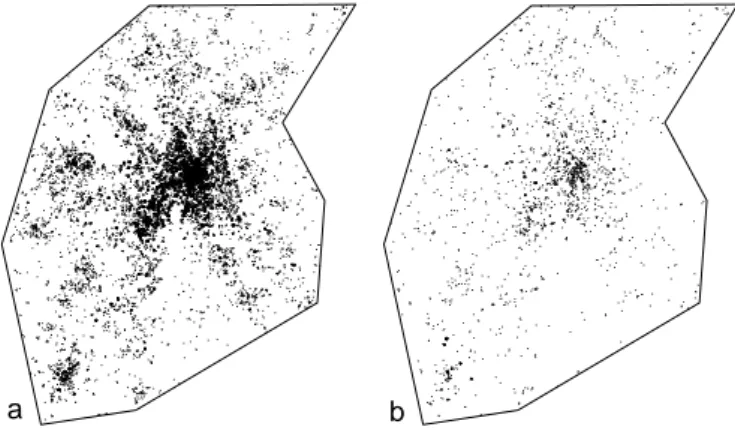
a b
Figure 1: Map of emergencies in the urban area of Toulouse, France, during year 2004 (about 33 km from south to north). (a) 20,820 emergencies have been recorded and mapped (many points are confused at the figure scale). (b) Locations of the 10 percent most serious ones.
Topographic functions require edge-effect corrections, provided by spatstat: The best cor-rection is systematically used. Relative functions ignore the window. Technical details are provided in the help files.
These functions return an ‘fv’ object, as defined in spatstat, which can be plotted.
3.2. Confidence envelopes
The classical confidence intervals, calculated by Monte Carlo simulations (Kenkel 1988) are obtained by the XEnvelope function, where X is the function’s name. Arguments are the number of simulations to run, the risk level, those of the function and the null hypothesis to simulate. These functions return a ‘dbmssEnvelope’ object which can be plotted.
Null hypotheses have been discussed by Goreaud and Pélissier (2003) for topographic func-tions such as K and byMarcon and Puech (2010) for relative functions. The null hypothesis for univariate functions is random position (points are drawn from a Poisson process for to-pographic functions) or random location (points are redistributed across actual locations for relative functions). Bivariate functions support random labeling and population indepen-dence as null hypotheses. The possible values of arguments are detailed in the help file of each function.
Building a confidence envelope in this way is problematic because the test is repeated at each distance. The underestimation of the risk has been discussed by Loosmore and Ford
(2006). Duranton and Overman(2005) proposed a global envelope computed by the repeated
elimination of simulations reaching an extreme value at any distance until the desired level is reached. The argument Global = TRUE is used to obtain it instead of the local one.
3.3. Examples
We illustrate the main features of the package by two examples. The first one comes from the economic literature (Bonneu 2007)1. A point pattern is induced by data about 20,820
1
The dataset can be downloaded from: http://publications-sfds.fr/index.php/csbigs/article/
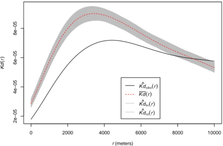
0 2000 4000 6000 8000 10000 2e−05 4e−05 6e−05 8e−05 r(meters) Kd ( r ) K d^ob s(r) K d(r) K d^h i(r) K d^l o(r)
Figure 2: Representation of Kd(r) values of the 10% most serious emergencies in year 2004
in the Toulouse urban area, showing their significant dispersion at all distances up to approx-imately 8 km. The solid, black curve is Kd. The dotted red curve is the average simulated value and the shaded area is the confidence envelope under the null hypothesis of random location. The risk level is 5%, 1000 simulations have been run. Distances are in meters.
emergencies involving the fire department of the urban area around Toulouse, France, during the year 2004 (Figure1). The workload associated to each emergency (the number of men × hours it required) is known. The original study tested the dependence between workload and location of emergencies: It did not exclude the null hypothesis of random labeling. We have a complementary approach here: We consider the 10 percent more serious emergencies, i.e., those which caused the highest workload. Kd may detect concentration (or dispersion) if, at
a distance r from a serious emergency, the probability to find another serious emergency is greater (or lower) than that of finding an emergency regardless of its workload:
R> load("CSBIGS.Rdata")
R> Category <- cut(Emergencies$M, quantile(Emergencies$M, c(0, 0.9, 1)), + labels = c("Other", "Biggest"), include.lowest = TRUE)
R> X <- wmppp(data.frame(X = Emergencies$X, Y = Emergencies$Y, + PointType = Category), win = Region)
R> KdE <- KdEnvelope(X, r = seq(0, 10000, 100), NumberOfSimulations = 1000, + ReferenceType = "Biggest", Global = TRUE)
R> plot(KdE)
The Emergencies data frame contains point coordinates (in meters) in columns X and Y and workload in column M. The second line of the code creates a vector containing a factor describing the workload to separate the 10% highest values. A ‘wmppp’ object is created then, containing the points and their mark. The KdEnvelope function is run from 0 to 10 km by steps of 100 m for the most serious emergencies. Figure 2 shows that the 10% most serious emergencies are more dispersed than the distribution of all emergencies. This opens the way to discuss on the optimal location of fire stations.
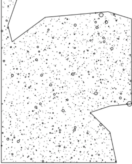
The second example uses the paracou16 point pattern (Figure 3) provided in the package. It represents the distribution of trees in a 4.1-ha tropical forest plot in the Paracou field
Figure 3: paracou16 point pattern. Circles are centered on trees in a 4.1-ha forest plot (the containing rectangle is 200 m wide by 250 m long). Circle sizes are proportional to the basal areas of trees.
station in French Guiana (Gourlet-Fleury, Guehl, and Laroussinie 2004). It contains 2426 trees, where the species is either Qualea rosea, Vouacapoua americana or Other (one of more than 300 species). Weights are basal areas (the area of the stems virtually cut 1.3 meter above ground), measured in square centimeters.
R> data("paracou16", package = "dbmss") R> plot(paracou16)
The question to test is dependence between the distributions of the two species of interest. Bivariate M (r) is calculated for r between 0 and 30 meters. 1000 simulations are run to build the global confidence envelope.
R> Envelope <- MEnvelope(paracou16, r = seq(0, 30, 2), + NumberOfSimulations = 1000, Alpha = 0.05,
+ ReferenceType = "V. Americana", NeighborType = "Q. Rosea", + SimulationType = "RandomLabeling", Global = TRUE)
R> plot(Envelope)
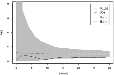
The calculated function (Figure4) is M, showing the repulsion between V. Americana and Q.
rosea up to 30 m. Significance is unclear, since the observed values of the function are very
close to the lower bound of the envelope. The complete study, with a larger dataset giving significant results, can be found in Marcon et al. (2012).
3.4. Goodness-of-fit test
A goodness-of-fit test for K has been proposed by Diggle (1983), applied to K byLoosmore
and Ford (2006) and to M by Marcon et al. (2012). It calculates the distance between
the actual values of the function and its average value obtained in simulations of the null hypothesis. The same distance is calculated for each simulated point pattern, and the returned
0 5 10 15 20 25 30 0 2 4 6 8 r(meters) M ( r ) M^ob s(r) M(r) M^h i(r) M^l o(r)
Figure 4: Representation of M (r) values of Qualea rosea around Vouacapoua Americana trees in the paracou16 point pattern. The solid, black curve is M. The dotted red curve is the average simulated value. The shaded area is the confidence envelope. M = 1 is expected if points are independently distributed. The risk level is 5%, 1000 simulations have been run. Distances are in meters.
p value of the test by the ratio of simulations whose distance is larger than that of the
real point pattern. The test is performed by the GoFtest function whose argument is the envelope previously calculated (actually, the function uses the simulation values). Applied to the example of Paracou trees, the p value is:
R> GoFtest(Envelope)
[1] 0.273
3.5. Ktest
The Ktest has been developed by Lang and Marcon (Lang and Marcon 2013;Marcon et al. 2013). It does not rely on simulations and returns the p value to erroneously reject CSR given the values of K. It relies on the exact variance of K calculated with edge-effect corrections. It only works in a rectangular window.
The following example tests a 1.5-ha subset of paracou16 (100 m by 150 m, origin at the South Western corner). It rejects CSR (p = 0.0027).
R> data("paracou16", package = "dbmss") R> RectWindow <- owin(c(300, 400), c(0, 150)) R> X <- paracou16[RectWindow] R> plot(X) R> Ktest(X, seq(5, 50, 5)) [1] 0.002682576
4. Conclusion
We built this package to provide an easy-to-use toolbox for users of spatial statistics mainly in economic geography and ecology. We wrapped up some spatstat functions to allow using them similarly to our original functions to build a rather complete set of tools, including to-pographic, absolute and relative functions. The analysis is limited to testing a point pattern against an appropriate null hypothesis, according to the framework developed in the eco-nomic literature (Combes et al. 2008) but we believe dbmss is a useful extension of spatstat for researchers who are motivated by empirical results more than by the tools themselves, regardless of their scientific field. Full features for point pattern analysis can be found in spatstat for those who wants to go further, including the simulation of many point processes as alternate null hypotheses and model fitting beyond exploratory statistics.
Future developments include the use of distance matrices as input of the distance-based functions to allow addressing road distance or geographic coordinates. We will also develop subsampling techniques to be able to manage huge datasets (several million points) whose distances cannot all be calculated in a reasonable time.
Acknowledgments
We thank Florent Bonneu who kindly allowed us to use his published fire emergency data. This work has benefited from an “Investissement d’Avenir” grant managed by Agence Na-tionale de la Recherche (CEBA, ref. ANR-10-LABX-25-01).
References
Baddeley A, Møller J, Waagepetersen R (2000). “Non- And Semi-Parametric Estimation of Interaction in Inhomogeneous Point Patterns.” Statistica Neerlandica, 54(3), 329–350. doi:10.1111/1467-9574.00144.
Baddeley A, Turner R (2005). “spatstat: An R Package for Analyzing Spatial Point Patterns.”
Journal of Statistical Software, 12(6), 1–42. doi:10.18637/jss.v012.i06.
Besag J (1977). “Comments on Ripley’s Paper.” Journal of the Royal Statistical Society B, 39(2), 193–195.
Bonneu F (2007). “Exploring and Modeling Fire Department Emergencies with a Spatio-Temporal Marked Point Process.” Case Studies in Business, Industry and Government
Statistics, 1(2), 139–152.
Bonneu F, Thomas-Agnan C (2015). “Measuring and Testing Spatial Mass Concentration of Micro-Geographic Data.” Spatial Economic Analysis, 10(3), 289–316. doi:10.1080/ 17421772.2015.1062124.
Combes PP, Mayer T, Thisse JF (2008). Economic Geography. Princeton University Press, Princeton.
Combes PP, Overman H (2004). “The Spatial Distribution of Economic Activities in the European Union.” In JV Henderson, JF Thisse (eds.), Handbook of Urban and Regional
Economics, volume 4, chapter 64, pp. 2845–2909. Elsevier, Amsterdam.
Diggle P (1983). Statistical Analysis of Spatial Point Patterns. Academic Press, London. Diggle P, Chetwynd A (1991). “Second-Order Analysis of Spatial Clustering for
Inhomoge-neous Populations.” Biometrics, 47(3), 1155–1163. doi:10.2307/2532668.
Duncan R (1991). “Competition and the Coexistence of Species in a Mixed Podocarp Stand.”
Journal of Ecology, 79(4), 1073–1084. doi:10.2307/2261099.
Duranton G, Overman H (2005). “Testing for Localisation Using Micro-Geographic Data.”
Review of Economic Studies, 72(4), 1077–1106. doi:10.1111/0034-6527.00362.
Duranton G, Overman H (2008). “Exploring the Detailed Location Patterns of UK Man-ufacturing Industries Using Microgeographic Data.” Journal of Regional Science, 48(1), 213–243. doi:10.1111/j.1365-2966.2006.0547.x.
Eddelbuettel D, François R (2011). “Rcpp: Seamless R and C++ Integration.” Journal of
Statistical Software, 40(8), 1–18. doi:10.18637/jss.v040.i08.
Ellison G, Glaeser E (1997). “Geographic Concentration in U.S. Manufacturing Industries: A Dartboard Approach.” Journal of Political Economy, 105(5), 889–927. doi:10.1086/ 262098.
Ellison G, Glaeser E, Kerr W (2010). “What Causes Industry Agglomeration? Evidence from Coagglomeration Patterns.” The American Economic Review, 100(3), 1195–1213. doi:10.1257/aer.100.3.1195.
Fortin MJ, Dale M (2005). Spatial Analysis. A Guide for Ecologists. Cambridge University Press, Cambridge.
Gini C (1912). Variabilità e Mutabilità, volume 3 of Studi Economico-Giuridici dell’Università
di Cagliari. Università di Cagliari.
Goreaud F, Pélissier R (2003). “Avoiding Misinterpretation of Biotic Interactions with the In-tertype K12-Function: Population Independence vs. Random Labelling Hypotheses.”
Jour-nal of Vegetation Science, 14(5), 681–692.
Gourlet-Fleury S, Guehl J, Laroussinie O (2004). Ecology & Management of a
Neotropi-cal Rainforest. Lessons Drawn from Paracou, a Long-Term Experimental Research Site in French Guiana. Elsevier, Paris, France.
Haase P, Pugnaire F, Clark S, Incoll L (1997). “Spatial Pattern in Anthyllis Cytisoides Shrubland on Abandoned Land in Southeastern Spain.” Journal of Vegetation Science, 8(5), 627–634. doi:10.2307/3237366.
Hoover E (1936). “The Measurement of Industrial Localization.” The Review of Economics
and Statistics, 18(4), 162–171. doi:10.2307/1927875.
Illian J, Penttinen A, Stoyan H, Stoyan D (2008). Statistical Analysis and Modelling of Spatial
Kenkel N (1988). “Pattern of Self-Thinning in Jack Pine: Testing the Random Mortality Hypothesis.” Ecology, 69(4), 1017–1024. doi:10.2307/1941257.
Lang G, Marcon E (2013). “Testing Randomness of Spatial Point Patterns with the Ripley Statistic.” ESAIM: Probability and Statistics, 17, 767–788. doi:10.1051/ps/2012027. Loosmore N, Ford E (2006). “Statistical Inference Using the G or K Point Pattern Spatial
Statistics.” Ecology, 87(8), 1925–1931. doi:10.1890/0012-9658(2006)87[1925:siutgo] 2.0.co;2.
Marcon E, Lang G, Traissac S, Puech F (2015). dbmss: Distance-Based Measures of Spatial
Structures. R package version 2.2.3, URLhttp://CRAN.R-project.org/package=dbmss. Marcon E, Puech F (2010). “Measures of the Geographic Concentration of Industries:
Im-proving Distance-Based Methods.” Journal of Economic Geography, 10(5), 745–762. doi: 10.1093/jeg/lbp056.
Marcon E, Puech F (2014). “A Typology of Distance-Based Measures of Spatial Concentra-tion.” Working Paper hal-00679993, HAL SHS. Version 2.
Marcon E, Puech F, Traissac S (2012). “Characterizing the Relative Spatial Structure of Point Patterns.” International Journal of Ecology, 2012(Article ID 619281), 1–11. doi: 10.1155/2012/619281.
Marcon E, Traissac S, Lang G (2013). “A Statistical Test for Ripley’s Function Rejection of Poisson Null Hypothesis.” ISRN Ecology, 2013(Article ID 753475), 1–9. doi:10.1155/ 2013/753475.
Openshaw S, Taylor P (1979). “A Million or so Correlation Coefficients: Three Experiments on the Modifiable Areal Unit Problem.” In N Wrigley (ed.), Statistical Applications in the
Spatial Sciences, pp. 127–144. Pion, London.
Penttinen A (2006). “Statistics for Marked Point Patterns.” In The Yearbook of the Finnish
Statistical Society, pp. 70–91. The Finnish Statistical Society, Helsinki.
Penttinen A, Stoyan D, Henttonen H (1992). “Marked Point Processes in Forest Statistics.”
Forest Science, 38(4), 806–824.
Picone G, Ridley D, Zandbergen P (2009). “Distance Decreases with Differentiation: Strategic Agglomeration by Retailers.” International Journal of Industrial Organization, 27(3), 463– 473. doi:10.1016/j.ijindorg.2008.11.007.
R Core Team (2015). R: A Language and Environment for Statistical Computing. R Founda-tion for Statistical Computing, Vienna, Austria.
Ripley B (1976). “The Second-Order Analysis of Stationary Point Processes.” Journal of
Applied Probability, 13(2), 255–266. doi:10.2307/3212829.
Ripley B (1977). “Modelling Spatial Patterns.” Journal of the Royal Statistical Society B, 39(2), 172–212.
Ripley B (1988). Statistical Inference for Spatial Processes. Cambridge University Press. doi:10.1017/cbo9780511624131.
Scholl T, Brenner T (2013). “Optimizing Distance-Based Methods for Big Data Analysis.”
Technical Report 2013-09, Philipps University Marburg.
Affiliation:
Eric Marcon, Stéphane Traissac AgroParisTech, UMR EcoFoG Campus agronomique, BP 316 97310 Kourou, French Guiana
E-mail: [email protected],[email protected] Florence Puech
RITM
Univ. Paris-Sud, Université Paris-Saclay 92330, Sceaux, France
E-mail: [email protected] Gabriel Lang
AgroParisTech, INRA, UMR 518 Math. Info. Appli. 16 rue Claude Bernard
75005 Paris, France
E-mail: [email protected]
Journal of Statistical Software
http://www.jstatsoft.org/published by the Foundation for Open Access Statistics http://www.foastat.org/ October 2015, Volume 67, Code Snippet 3 Submitted: 2012-12-17