Analysis of a simplified calibration procedure
for 18 design-phase building energy models
The MIT Faculty has made this article openly available.
Please share
how this access benefits you. Your story matters.
Citation
Samuelsona, Holly W., Arash Ghorayshib and Christoph F. Reinhart.
“Analysis of a simplified calibration procedure for 18
design-phase building energy models.” Journal of building performance
simulation, vol. 9, no. 1, 2015, pp. 17–29 © 2015 The Author(s)
As Published
10.1080/19401493.2014.988752
Publisher
Informa UK Limited
Version
Author's final manuscript
Citable link
https://hdl.handle.net/1721.1/126642
Terms of Use
Creative Commons Attribution-Noncommercial-Share Alike
Analysis of a Simplified Calibration Procedure for 18 Design-Phase Building Energy Models
Holly W. Samuelson
a, #, Arash Ghorayshi
b, and Christoph F. Reinhart
ca
Harvard University, Graduate School of Design, 48 Quincy Street, Cambridge, MA 02138 USA
b
MMM Group Ltd., formerly Enermodal Engineering, 582 Lancaster Street West, Kitchener, ON
N2K 1M3 Canada
c
Massachusetts Institute of Technology, Department of Architecture, 77 Massachusetts
Avenue, Cambridge MA 02139, USA
#
Corresponding author. email address: hsamuelson@gsd.harvard.edu
Abstract
This paper evaluates the accuracy of 18 design-phase building energy models, built according to LEED Canada protocol, and analyzes the effectiveness of model calibration steps to improve simulation predictions with respect to measured energy data. These calibration steps, applied in professional practice, included inputting actual weather data, adding unregulated loads, revising plug-loads (often with submetered data), and other simple updates. In net, the design-phase energy models under-predicted the total measured energy consumption by 36%. Following the calibration steps, this error was reduced to a net 7% under-prediction. For the monthly Energy Use Intensity (EUI) the coefficient of variation of the root mean square error improved from 45% to 24%. Revising plug-loads made the largest impact in these cases. This step increased the EUI by 15% median (32% mean) in the models. This impact far exceeded that of calibrating the weather data, even in a sensitivity test using extreme weather years.
Keywords: energy simulation, plug-loads, process loads, unregulated loads, weather, design-phase models, compliance models
1. Introduction
Commercial buildings are complicated thermodynamic objects. Occupant behavior and local weather conditions may strongly impact their energy use, making it difficult to detect operational inefficiencies such as malfunctioning equipment and inefficient control strategies. Unfortunately, such inefficiencies are ubiquitous and waste substantial energy and money. A study of 60 buildings by Lawrence Berkeley National Laboratory showed that, before intervention, at least half had problems with their system controls, a minimum of 40% had faulty HVAC equipment, and 25% or more had problems with specific "green" HVAC features (Piette, Nordman, & Greenberg, 1994). One group of researchers estimated that finding and fixing these types of problems can save $18 billion or more per year in commercial buildings in the U.S. alone (Mills et al., 2004).
Fortunately, researchers have shown that state-of-the-art computer-based energy simulation can aid in the search for operational problems in processes such as existing-building commissioning (Adam, Andre,
Aparecida Silva, Hannay, & Lebrun, 2004; Andre, Cuevas, Lacote, & Lebrun, 2003) and
ongoing-commissioning (O'Neill et al., 2011; Song, Liu, Claridge, & Haves, 2003). Carling, Isakson, and Blomberg (2004) demonstrated the value of whole-building energy simulation to support new building energy commissioning. At the same time they noted that their procedure was too expensive for routine
application as preparing the detailed model took several weeks. This situation helps explain why, despite advances in research, practitioners rarely use energy simulation beyond a building's design-phase (Claridge, 2011). The post-occupancy task of measurement and verification (M&V) is an occasional exception. While an established M&V methodology exists which uses a calibrated energy model to isolate the impact of installed energy conservation measures, even its proponents caution that the methodology "is best applied where… the budget for M&V is generous." (Efficiency Valuation
Organization, 2006). A key obstacle to the use of simulations during building operation is hence the cost of generating an energy model to start.
This obstacle may become less relevant for many projects as building energy codes and green building standards, such as the UK's Building Regulations Part L (Stationery Office London, 2010), California’s Title 24 (California Energy Commission, 2007), and LEED (US Green Building Council, 2009) promote and/or require the wider spread use of building energy modeling during building design. Could these design-phase energy models then be used to improve building operations?
The answer is, "probably not directly", since researchers have shown design-phase models to often be poor predictors of actual energy use in buildings (Ahmad & Culp, 2006). In fact, ASHRAE 189.1
specifically alerts the reader that design-phase energy models may substantially diverge from actual building energy use “due to variations such as occupancy, building operation... energy use not covered by this procedure...” etc. (ANSI, ASHRAE, USGBC, & IES, 2010). However, despite these well-known facts regarding model accuracy, in a recent survey of 116 energy modelers 75% believed that (once
(Samuelson, Lantz, & Reinhart, 2012). Given this optimism within the energy simulation community, the question becomes, what shortcomings of design-phase models can be improved with calibration steps? Model calibration can be time-consuming and has been described as "an art form that inevitably relies on user knowledge… and an abundance of trial and error" (Reddy, 2006). Various researchers have advanced the calibration process (Clarke, Strachan, & Pernot, 1993; Haberl & Bou-Saada, 1998; Pan, Huang, & Gang, 2007; Reddy, 2006) and developed time-saving techniques, especially for use with hourly-measured data. The greater the granularity of measurements, in terms of time steps and end uses, the more accurate the calibration procedure can be. For instance, a widely researched calibration method called signature analysis,involves analyzing the fit between simulated and measured hourly data to deduce the necessary model adjustments (G. Liu & Liu, 2011; M. Liu et al., 2003; M. Liu, Liu, Claridge, & Haberl, 2006; Wei, Liu, & Claridge, 1998). Practitioners with less granular information, such as monthly metered data only, face additional challenges. Other problems that modelers face during calibration is that most simulation packages rely on significant approximations of HVAC systems (Bannister, 2009). Finally, design-phase models pose unique challenges, since practitioners built these models when many model inputs were yet unknown and with the intent of comparing design options or demonstrating code compliance rather than predicting absolute energy consumption.
In this study the authors describe and examine the effectiveness of a simple, heuristic calibration procedure for design-phase energy models that has been used over several years in the second author’s sustainable consultancy practice in projects for which the firm was hired as the energy modeler during design as well as the commissioning agent during the first year of building operation. In their latter capacity the firm uses the calibration procedure to help ensure that a building functions as intended. The calibration procedure is evidence-based in the spirit of Raftery, Keane, and O'Donnell (2011), in that the modelers only update input parameters based on more reliable evidence, such as direct
following, the ability of the different calibration steps to increase simulation accuracy is evaluated for 18 buildings and recommendations are made for others interested in adopting a comparable process in their practice.
2. Methodology
2.1 The Dataset
The authors analyzed a set of 18 commercial building projects located within 100 km (60 miles) of Toronto, Ontario. For each project, modelers from the earlier mentioned energy consulting firm had built the energy models to support the new building design process and to document energy
conservation measures for LEED Canada New Construction or Core and Shell version 1.0 certification (Canada Green Building Council, 2007). The modelers then "partially-calibrated"the models, typically over the first year of occupancy, to inform the measurement and verification (M&V) and extended commissioning process. Here the authors use the term "partial-calibration" to describe the act of bringing the energy model inputs closer to as-operated conditions, while recognizing that the modelers could have calibrated the models further with additional effort.
The authors started the investigation with all 34 of the firm's model/calibration projects with at least one year of monthly measured utility data available at the time. The ten different modelers who had built these models had not documented their projects with the idea that future researchers would recreate their work. Therefore, nine projects needed to be eliminated due to inadequate
documentation. The authors also removed another seven models that were built in software packages other than EE4, a DOE2.1 based simulation program used to demonstrate compliance with LEED Canada (Canada Green Building Council, 2007), in order to streamline the time-intensive analysis process across the remaining 18 cases.The authors manually reran the models for each calibration step in order to validate the original calibration process.
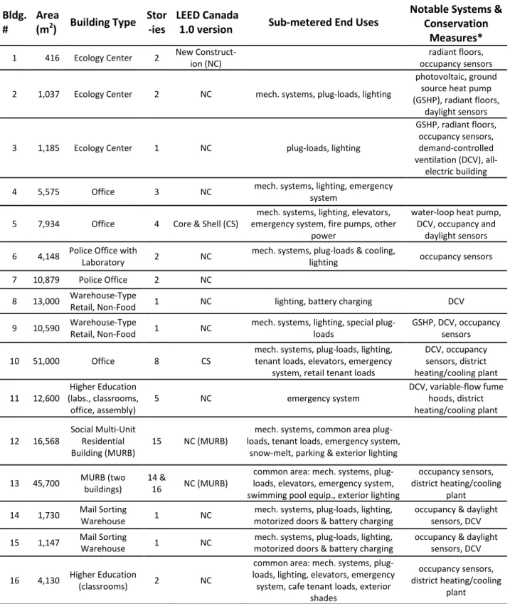
All 18 case studies were new buildings, completed between 2008 and 2012 and then monitored for at least 12 months. The buildings ranged in size from 416 m2 (4480 ft2) – 51,000m2 (550,000ft2) and one to
16 stories. Table 1 provides more project information.
Table 1: Characteristics of Building Cases
Bldg. # Area (m2) Building Type Stor -ies LEED Canada
1.0 version Sub-metered End Uses
Notable Systems & Conservation
Measures*
1 416 Ecology Center 2 New
Construct-ion (NC)
radiant floors, occupancy sensors 2 1,037 Ecology Center 2 NC mech. systems, plug-loads, lighting
photovoltaic, ground source heat pump (GSHP), radiant floors,
daylight sensors
3 1,185 Ecology Center 1 NC plug-loads, lighting
GSHP, radiant floors, occupancy sensors, demand-controlled ventilation (DCV), all-electric building
4 5,575 Office 3 NC mech. systems, lighting, emergency
system
5 7,934 Office 4 Core & Shell (CS)
mech. systems, lighting, elevators, emergency system, fire pumps, other
power
water-loop heat pump, DCV, occupancy and
daylight sensors 6 4,148 Police Office with
Laboratory 2 NC
mech. systems, plug-loads & cooling,
lighting occupancy sensors
7 10,879 Police Office 2 NC
8 13,000 Warehouse-Type
Retail, Non-Food 1 NC lighting, battery charging DCV
9 10,590 Warehouse-Type
Retail, Non-Food 1 NC
mech. systems, lighting, special plug-loads
GSHP, DCV, occupancy sensors
10 51,000 Office 8 CS
mech. systems, plug-loads, lighting, tenant loads, elevators, emergency
system, retail tenant loads
DCV, occupancy sensors, district heating/cooling plant 11 12,600 Higher Education (labs., classrooms, office, assembly) 5 NC emergency system DCV, variable-flow fume hoods, district heating/cooling plant 12 16,568 Social Multi-Unit Residential Building (MURB) 15 NC (MURB)
mech. systems, common area plug-loads, tenant plug-loads, emergency system,
snow-melt, parking & exterior lighting
13 45,700 MURB (two buildings)
14 &
16 NC (MURB)
common area: mech. systems, plug-loads, elevators, emergency system, swimming pool equip., exterior lighting
occupancy sensors, district heating/cooling
plant 14 1,730 Mail Sorting
Warehouse 1 NC
mech. systems, plug-loads, lighting, motorized doors & battery charging
occupancy & daylight sensors, DCV 15 1,147 Mail Sorting
Warehouse 1 NC
mech. systems, plug-loads, lighting, motorized doors & battery charging
occupancy & daylight sensors, DCV 16 4,130 Higher Education
(classrooms) 2 NC
common area: mech. systems, plug-loads, lighting, elevators, emergency
system, cafe tenant loads, exterior shades
occupancy sensors, district heating/cooling
17 18,013 Luxury MURB (two buildings)
10 &
8 NC (MURB)
common area: mech. systems, plug-loads, elevators, exterior & parking
lighting
district heating/cooling plant 18 27,000 Office/Call Center 10 CS mech. systems, plug-loads, lighting,
emergency system occupancy sensors *All buildings have energy recovery ventilation. All buildings have a natural gas fired boiler, unless otherwise noted. Occupancy sensors, where listed, are part of the lighting control.
To understand how these cases compare to other LEED-certified projects, Figure 1 shows the measured versus predicted Energy Use Intensity (EUI) of the 18 case studies alongside a dataset from Turner and Frankel (2008), which consists of LEED (US) Version 2 (US Green Building Council, 2001) certified buildings completed between 2001 and 2007.1
The Canadian cases have a slightly higher median EUI of 244 kWh/m2 compared to 198 kWh/m2 for the
Turner and Frankel cases. However, model accuracy was similar in both groups; the design-phase simulation predictions deviated by 31% median from the measured EUI for the Canadian buildings compared to 36% in the older study.
Figure 1: Current Cases Shown in Context
2.2 Modeling Protocol and Software
In the current cases, the energy modelers originally followed the Performance Compliance for Buildings (National Research Council Canada, 1999) protocol, which Canadian practitioners use to demonstrate compliance with the Model National Energy Code for Buildings (MNECB) for Commercial Building Incentive Program compliance (Candian Commission on Building and Fire Codes, 1997) and LEED Canada 1.0. Per the MNECB/LEED compliance process, the models are peer-reviewed, which may help improve the pre-calibration model quality, and modelers follow a detailed modeling procedure that creates more consistency between models than would otherwise be the case. The modelers used the EE4 version 1.7 software (Natural Resources Canada, 2005), based on the DOE2.1E simulation engine2 (J. J. Hirsch &
Regents of the University of California, 1999) which references DOE-2 hourly .bin format weather files. Importantly, the Performance Compliance protocol encourages modelers to use default values,
according to building type, for the following loads: number of occupants, receptacle power, service water heating, outdoor air requirements, space temperature schedule, and
occupancy/lighting/operation schedules. Modelers can, however, add special loads/heat gains as an additional input. EE4 contains a library of input selections related to the loads above. These values can be over-written, but the onus then falls on the modeler to document non-standard conditions.
The EE4v1.7 software itself poses limitations for the prediction of absolute energy performance. For example, it lacks the capacity to model the following features: shading/reflection from vegetation or neighboring buildings, exterior lights, elevator usage, and steam humidifiers (Natural Resources Canada Office of Energy Efficiency & CANMET Energy Technology Centre, 2008) as well as special equipment
2
The authors have made available the custom Python scripts created for this research to batch process DOE (.sim) results files and extract key monthly and annual results. These scripts may be helpful to EE4, eQuest, and other .sim file users. The public can download them here:
whose energy use is not regulated by the code/incentive program. With the exception of
vegetation/neighboring buildings, the modelers added loads from missing features as part of the calibration process.
2.3 The Calibration Method
The modelers performed a series of steps to improve the accuracy of the models with reasonable effort, ensuring that each revised input came from a more reliable source than the original input, as noted above. In some cases, the modelers made adjustments within the energy model, i.e. the EE4 software interface. In other cases, the modelers post-processed the simulation results in a spreadsheet, for example replacing simulated with sub-metered plug-loads. This external approach overcame two hurdles. First, it allowed the modelers to add loads from building features, such as exterior lights, that the software interface could not support. Second, it allowed the modelers to overcome a discrepancy between the building's coarsely zoned sub-metering systems and the finely-zoned model geometry.3
The benefits and shortcomings of this external calibration approach will be discussed in Section 4.1.
2.4 Analysis Procedure
2.4.1 Overview
The original modelers performed the calibrations in an ad hoc fashion, for example inputting three-months of actual weather data while simultaneously changing the occupancy schedules. This process prohibited the authors from ascertaining which calibration tasks substantially affected the simulations. Therefore, the authors reran all simulations and systematically isolated each step. The authors made
3 The modelers followed the EE4 modeling protocol (Natural Resources Canada Office of Energy
Efficiency & CANMET Energy Technology Centre, 2008) building zoning principles, thereby creating separate model zones per HVAC system, space operation/function, heating/cooling loads, and solar orientation.
minor revisions to the modelers' original approaches if they suspected an error or if expanded sub-metered data became available.
The starting point for each case was the "design-phase model", i.e. the energy model submitted to demonstrate compliance with the LEED energy credits. For analysis, the authors divided the calibration steps into categories, described in sections 2.4.2 and 2.4.3. The authors changed one category of inputs at a time and, after each step, identified the net change from the previous model’s results.
2.4.2 Weather
The authors compared simulation results using typical versus historical weather data corresponding to the building metering periods. The modelers/authors used typical weather data included in the EE4 library, originating from the Canadian Weather for Energy Calculations (CWEC) database, an
amalgamation of 1960-1991 weather data. They obtained the historical weather data from the National Climate Data and Information Archive and formatted it for use in DOE2.1E using the DOEWTH.exe converter (J. J. Hirsch & Regents of the University of California, 1999). Since this historical data did not include solar radiation information, a common problem, the modelers used solar radiation data from the CWEC typical weather file, a known modeling inconsistency. The weather converter uses monthly average clearness, which the modelers estimated from the hourly CWEC horizontal irradiance and monthly average extraterrestrial radiation for the latitude, per Duffie and Beckman (1991).
The authors also performed a sensitivity analysis to investigate the effect of calibrating weather inputs in extreme weather years. Crawley (2008a, 2008b) investigated the impact of historical weather data from 1961 to 1999 on the annual simulation results of multiple test buildings in various cities including Toronto. He found that 1998 and 1972 resulted in the lowest and highest simulated energy consumption respectively in his Toronto cases. Therefore the authors used 1998 and 1972 Toronto weather data (Environment Canada, 2001) in their sensitivity analyses.
Due to the known modeling inconsistency with the solar radiation data in the original calibration procedure, the authors performed a second sensitivity analysis to understand the potential impact of solar inputs on resulting simulated energy consumption. The 1998 and 1972 weather files (Environment Canada, 2001) did include solar radiation data (albeit modeled data, since measured historic radiation data is rare.) The authors performed simulations first using the unadulterated 1998 and 1972 weather data and then exchanging the solar radiation inputs for values taken from the CWEC typical weather file. 2.4.3 Plug-Loads, Unregulated Loads, and Other Calibration Categories
The authors used the historical weather data when testing the remaining calibration steps. They broke these steps into the following categories: HVAC equipment, HVAC operation schedule, occupant density/schedule (also called occupancy), lighting, infiltration, plug-loads, and unregulated loads. The lighting category included any changes to the installed lighting power density, controls, or schedules. The plug-loads category included revisions to energy use from office equipment, home appliances, and other equipment related to the occupants' business or activity, as listed in Section 3.2. In all cases, the modelers included plug-load estimates in the design-phase models. In many cases they used the MNECB default values for plug-load densities and operating schedules, as described in Section 2.2, which they revised during calibration. In contrast, the “unregulated loads” category included loads that the modelers excluded from the design-phase model, because they are unregulated by the code/incentive protocol and excluded from the EE4 software interface. This category included exterior lights and other building equipment listed in Section 3.3.
3. Results
3.1 Overview
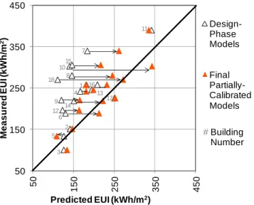
The “goodness-of-fit” between measured and predicted results improved substantially with the partial-calibration, as illustrated in Figure 2. In net, the design-phase energy models under-predicted the
measured energy consumption for all 18 buildings by 36%. Following calibration, this error decreased to a net 7% under-prediction. The annual mean bias error improved from -28% to -9%. The maximum difference between measured and simulated annual energy use for any building reduced from 59% to 34%. Using the formulas shown in Equation 1, the accuracy also improved in terms of monthly
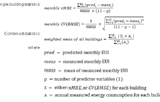
normalized mean bias error (nMBE) and coefficient of variation of the root mean square error CV(RMSE), from 41% to 18% and 45% to 24% respectively.
Aggregate statistics like these can help the modelers evaluate the overall effectiveness of their modeling and calibration practices. These numbers suggest that the partial-calibration process helped rectify the discrepancy, but some noteworthy building energy use remained unexplained by the models. Trends such as the pervasive design-phase under-predictions may indicate that the modelers need to adjust their future design-phase assumptions. The following analysis helps deduce which design-phase inputs may be the most problematic.
Figure 2: Goodness-of-fit: Design-Phase Models vs. Partially-Calibrated Models
16 2 3 4 6 7 8 9 10 11 12 15 18 5 13 14 1 17 50 150 250 350 450 50 150 250 350 450 M e a s u re d E U I ( k W h /m 2) Predicted EUI (kWh/m2) Design-Phase Models Final Partially-Calibrated Models #Building Number
Equation 1: Error Statistics
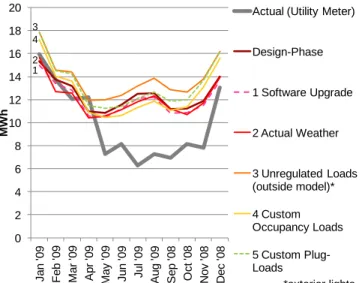
Figure 3 shows examples of the step-by-step calibration process for Building 8, a warehouse-type, or "big box" store. The authors included this particular case because it most clearly delineates the process from one step to another. In contrast, Figure 4 shows the same data for Building 3, an ecology center, which had the highest error statistics and least improvement with calibration. These results illustrate that the process did not always improve the model's goodness-of-fit.
(b) Monthly Electricity
(c) Monthly Natural Gas
Figure 3 a-c: The calibration steps for Building 8, a warehouse-type store
0 50 100 150 200 250 300 350 Ja n '0 9 F e b '0 9 Ma r '0 9 Ap r '0 9 Ma y '0 9 Ju n '0 9 Ju l ' 0 8 Au g '0 8 Se p '0 8 O ct '0 8 N o v '0 8 D e c '0 8 MW h Actual (Utility Meter) Design-Phase 1 Actual Weather 2 Custom Lighting Schedules 3 Custom Plug-Load Schedules 4 Sub-Metered Plug-Loads* (outside model) 5 Unregulated Loads** (outside model)
* retail displays, battery charging for forklifts ** exterior lights
1 2 3 4 5 0 20 40 60 80 100 120 140 160 Ja n '0 9 F e b '0 9 Ma r '0 9 Ap r '0 9 Ma y '0 9 Ju n '0 9 Ju l ' 0 8 Au g '0 8 Se p '0 8 O ct '0 8 N o v '0 8 D e c '0 8 MW h Actual (Utility Meter) Design-Phase 1 Actual Weather 2 Custom Lighting Schedules 3 Custom Plug-Load Schedules No change to gas with calibration steps 4-5 1 2 3 95 105 115 125 135 145 95 105 115 125 135 145 Me a s u re d EU I (k W h /m 2) Predicted EUI (kWh/m2) 0 Design-Phase Model 1 Software Upgrade 2 Actual Weather 3 Unregulated Loads* 4 Custom Occupant Density/ Schedules 5 Custom Plug-Loads 0 1,2 4 3 Unpredicted Energy Savings: 5
(a) EUI
(b) Monthly Electricity (all electric building)
Figure 4 a-b: Calibration steps for Building 3, an ecology center
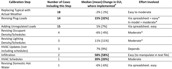
Figures 9-11 show the results of each calibration step for each building compared to measured electricity and natural gas consumption. The authors list the changes included in the most notable calibration steps. Table 2 lists each calibration step and indicates in how many cases the modelers implemented that step. The authors also calculated the median impact of the step, where implemented, and evaluated the relative effort involved in the calibration step (excluding data gathering.)
The modelers implemented three calibration steps in most of the cases --namely, updating plug-loads, adding unregulated loads, and replacing CWEC data with historical weather data, since revised values for these inputs were readily obtainable. Therefore, for the group as a whole, those three relatively easy steps accounted for the majority of the model improvement. The modelers implemented other
calibration steps only on a limited portion of the cases, i.e. the specific cases where more accurate inputs were available and the modelers believed that their impact would warrant the effort. For example, the modelers had no additional information regarding infiltration rates. Therefore, they kept the original infiltration rates except in two special cases where they had reason to suspect significant problems with the default assumptions, such as the case described in Section 3.5.
0 2 4 6 8 10 12 14 16 18 20 Ja n '0 9 F e b '0 9 Ma r '0 9 Ap r '0 9 Ma y '0 9 Ju n '0 9 Ju l ' 0 9 Au g '0 9 Se p '0 8 O ct '0 8 N o v '0 8 D e c '0 8 MW h
Actual (Utility Meter)
Design-Phase 1 Software Upgrade 2 Actual Weather 3 Unregulated Loads (outside model)* 4 Custom Occupancy Loads 5 Custom Plug-Loads *exterior lights 1 2 3 4
Table 2: The Calibration Steps Implemented, their Impact, and the Effort Involved
Calibration Step Number of Cases
Including this Step
Median [mean]Change in EUI, where implemented4
Effort Involved Replacing Typical with
Actual Weather 18 -2% [-2%] Easy to moderate
Revising Plug-Loads 14 15% [32%] Via spreadsheet = easy*
In model = moderate*
Adding Unregulated Loads 15 5% [7%] Via spreadsheet. easy
Revising Occupant
Density/Schedules 4 -6% [-4%] Moderate*
Revising Lighting
Density/Schedules 3 11% [11%] Moderate*
HVAC Updates (not
including schedules) 3 7% [9%] Depends
Infiltration 2 58% [58%] Easy (to manipulate in text file)
HVAC Schedules 1 20% [20%] Moderate
Revising Domestic Hot
Water 1 -6% [-6%] Via spreadsheet. easy
* if information is available. The effort level varies. More zones in model = more effort.
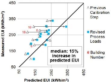
3.2 Updating Plug-Loads
The modelers produced the biggest overall calibration impact, by far, by revising the plug-loads. As shown in Figure 5, they implemented this step in 14 cases which increased the predicted EUI by 15% median (32% mean). Revised plug-loads included the following: miscellaneous occupant equipment loads (in 13 cases), computer servers (in two cases), laboratory equipment, broadcast equipment, retail displays, battery charging stations, communal laundry, and café equipment (in one case each). They used monthly sub-metered data unless otherwise noted. As can be seen in Figure 5, the plug-loads decreased slightly (2% and 7%) in only two (warehouse-type) buildings and increased considerably in four notable cases. In Buildings 10 and 18, both large core-and-shell office buildings, the modeler assumed typical office functions using MNECB default loads and schedules. After construction, Buildings
10 and 18 housed more energy-dense functions including a call center and a broadcast station respectively. Both cases resulted in much higher monthly sub-metered than predicted plug-loads. In Building 6, police offices, the monthly sub-metered forensic laboratory loads proved to be much higher than modeled. In Building 8, a warehouse store, the modeler ultimately added missing loads from retail displays (estimated from short-term measurement) and battery charging stations for equipment such as forklifts (sub-metered). Revising the plug-loads in these four buildings increased the EUI by 145%, 142%, 48%, and 32% respectively.
Figure 5: Effect of Revising Plug-Loads
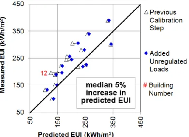
3.3 Adding Unregulated Loads
The modelers added unregulated loads in all but three cases. Considering the group as a whole, this calibration step made the second largest impact on the predicted EUI. The modelers added loads from exterior or parking lighting (calculated via installed lighting power and predicted hours of operation) in 15 cases, resulting in a median EUI increase of 4% (5% mean). The modelers similarly added missing elevator loads (estimated based on measurements from a benchmark building) in eight cases, resulting in a median EUI increase of 1% (1% mean). They also added estimated or metered loads from security equipment, emergency equipment, pool heating, motorized doors, and a snow-melt system (1 case each). In total, the modelers added unregulated loads in 15 cases, which increased the EUI by a median
of 5% (7% mean) as shown in Figure 6. The largest impact (32% increase in EUI) from this step occurred in Building 12, a multi-unit residential building, when the modeler added monthly metered loads from a large parking facility.
Figure 6: Effect of Adding Unregulated Loads
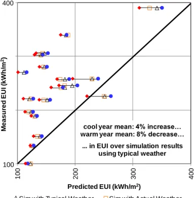
3.4 Updating Weather Inputs
The modelers replaced the CWEC weather data with historical data in all 18 cases, which decreased the EUI by a median of 2% (2% mean). The years 2008-2012 were all warmer than average in Toronto (Environment Canada, 2001), and in this heating-dominate climate, in all but two cases, the updated weather data resulted in lower simulated energy use. Contrary to expectations, calibrating the weather data generally increased the discrepancy between measured and simulated energy use, both annually and monthly, because the less-accurate weather data partially counteracted other inaccuracies in the model at that point in the calibration.
Figure 7 shows the results of these weather calibrations as well as the sensitivity analysis using Toronto extreme weather years, as described in Section 2.4.2. Compared to the CWEC data, the extreme cool year had -18% cooling degree days (CDD) and +23% heating degree days (HDD), whereas the extreme warm year had +20% CDD and -25% HDD. Despite this wide variability, the cool and warm extreme years
resulted in only a 4% increase and 8% decrease respectively in median simulated EUI (4% and 8% mean) across the 18 cases, compared to the typical-weather year. These results give some indication of the effect that weather calibration could make in more extreme years. One should note that this low effect of weather on the 18 buildings is a testament to their high quality thermal envelopes. The number would very likely be larger for more standard Canadian buildings. In the analysis of solar radiation data in the extreme years, as described in Section 2.4.2, the change in solar radiation data produced a 1% median (1% mean) change in EUI over the 18 cases.
Figure 7: Weather Sensitivity Analysis
3.5 Other Calibration Steps
This section includes the highest-impact cases for each of the remaining calibration categories. In Building 14, a mail sorting warehouse, revising the infiltration rate to consider the often-open loading dock doors made a substantial impact, increasing the simulated EUI by 75%. The modeler calculated the new infiltration rate by hand based on opening sizes. Therefore, the value is still estimated but based on
100 200 300 400 M e a s u re d E U I (k W h /m 2) Predicted EUI (kWh/m2)
Sim with Typical Weather Sim with Actual Weather Sim with 1972 Weather Sim with 1998 Weather
cool yearmean: 4% increase…
warm year mean: 8% decrease… ... in EUI over simulation results
using typical weather 100
more information than the default assumption. In Building 18, an office/call center described above, revising the HVAC operation schedules, based on an interview with the building manager, increased the EUI by 20%.The installed HVAC equipment differed from the design-phase assumptions in Building 7, a police office. This change increased the predicted EUI by 19%. In Building 8, a warehouse store, the modelers revised the lighting schedules, based on short-term measurements, resulting in a 19% increase in EUI. Conversely in Building 3, an ecology center, their revised occupancy schedules, based on an interview with the building owner, decreased the EUI by 9%.
4. Discussion and Outlook
4.1 Partial Model Calibration
The previous section revealed that the straightforward and low-effort partial-calibration process described above reduced the annual and monthly mean bias errors between measured and simulated energy use in 18 building by more than 50% compared to using the original design-phase models. This finding is both important and encouraging and the authors recommend that design teams and owners adopt a version of this procedure to improve their compliance-type models.5 It is important to note that
the 18 case study projects did not receive any additional research funding to support the calibration process described. This demonstrates that partial model calibration can, in fact, be conducted in a for-profit context.
In these cases, like many compliance-type models, design-phase inputs did not match the realities of the as-occupied/as-operated building, and unregulated loads were not included in the original models. Here, revising the plug-loads generally created the largest impact followed by adding unregulated loads. Both steps required relatively little effort. In some cases, the modelers implemented a spreadsheet shortcut for updating these loads. In those cases, they minimized the calibration effort but excluded the
interrelated effects of the revised load on other systems in the model.6 Even so, this spreadsheet
approach could be a cost-effective initial calibration step that the modeler could replace with a more exacting approach later if desired.
4.2 Remaining Inaccuracies
As discussed, the partial-calibration did not correct all model inaccuracies. Parameters which were not monitored here should not be considered insignificant. For example, researchers have shown that the typical approach to estimating window U-factors used here, based on standard test dimensions rather than actual window sizes, may be inaccurate (A. Hirsch, Pless, Guglielmetti, & Torcellini, 2011). Software limitations also remained unaddressed.Notably, modelers in EE4 cannot model Demand Controlled Ventilation (DCV) and instead implement a work-around, described in the EE4 manual, to reduce the fan operating hours and thus the amount of outside air being heated or cooled. As shown in Table 2, eight of the studied buildings include DCV. The DOE2 engine also poses challenges to accurately representing ventilation energy recovery (ERV) by restricting one's ability to model upstream preheat coils and reducing the ERV effectiveness to a single number which may not be accurate under all control situations. All 18 buildings included ERV. Furthermore, researchers have also shown that DOE2 may overestimate boiler efficiency at low loads (Kenna & Bannister, 2009). Twelve cases had boilers. The authors recommend using a more flexible software package for future modeling and calibration efforts. 4.3 Accuracy of Compliance Models
A sobering takeaway from these case studies is that the difference between simulated and measured energy use in certified green buildings is actually quite large, with a median of 31% for the whole group and reaching as high as 59% in the worst case. This study shows that routinely-voiced expectations that
6 For example, in Building 8 the added retail displays not only consumed electricity directly, which the modeler tallied in the spreadsheet, but also added heat to the space, which would be ignored with this method.
future energy use can be predicted to within 10% to 20% during design should be upwardly adjusted. Notably, the bulk of these discrepancies was not caused by the simulation algorithms, the availability of good weather data, or the modelers’ ability to reliably model building envelope properties. The main discrepancies were rather a result of the compliance modeling protocols as well as how buildings are used and operated, which to some extent could be anticipated in the design-phase. For example, in Building 1, a small ecology center and the building most impacted by weather variation, switching from the 1998 (extreme warm year) to 1972 (extreme cool year) weather increased the annual EUI by 23%. This is large effect, but it nevertheless pales in comparison to the impact of revising the plug-loads in Buildings 10 and 18, which increased the EUI by over 140% in each case.
Modeling protocols in North America require the modeler to compare his/her as-designed building to a code-compliant baseline model, identical to the former except for the energy conservation measures. This approach penalizes designers for high loads that fall outside of their design control. This partially explains why modeling protocols traditionally excluded certain loads or deemphasized custom plug-load inputs, and why some modelers may hesitate to over-estimate these loads. The 5% median increase caused by adding unregulated loads found in this study further underscores the need to include all loads in the design-phase model, if possible. Policy-makers have begun requiring modelers to include custom plug-load and other miscellaneous load predictions in the model (ASHRAE & IESNA, 2010) in an effort to take a more comprehensive view of energy performance and to bring compliance-type model
predictions closer to reality. More research is needed to determine whether modelers are actually capable of predicting these loads accurately in the design-phase.
4.4 Building Sub-metering
Where installed, building sub-metering provided valuable data for calibration. Nevertheless, in this research, sub-metering seldom supplied data in the desired level of detail for input into the model. Translating the coarse-grained measured data into more granular end-uses and building zones required
effort and judgment. Software developers can help address this difficulty. In addition, the practice of building sub-metering may grow more prevalent and granular with the increasing affordability of equipment (Claridge, 2011) and the influence of codes and standards (ANSI et al., 2010; US Green Building Council, 2009), which in turn will decrease the calibration effort level even further. 4.5 Calibration Triage
In these cases, the remaining predicted versus measured energy discrepancies helped guide the search for operational problems in the buildings. For example, according to the commissioning agent for Building 8, shown in Figure 3, the simulation helped uncover a problem with the building automation system, a fault in the energy recovery ventilation equipment, and unintentional off-hours lighting. Higher quality models and calibrations would help project teams uncover more operational problems like these, but at an increased cost. The ASHRAE 14 standard (ASHRAE, 2002) lists goodness-of-fit suggestions for calibrated models. In these 18 cases, none of the final, partially-calibrated simulations met all of the ASHRAE 14 suggestions. On one hand, higher quality models and calibrations may have uncovered more building problems and provided value for other applications such as on-going commissioning. On the other hand, building owners may hesitate to invest in an extensive model calibration process to start the investigation, since the process might not lead to remunerable savings if the building already performs generally as it should.A coarse first-pass calibration approach can provide a cost-effective means to identify projects that warrant further calibration effort, just as triage helps to prioritize care in a hospital emergency room.
The simulated/measured discrepancy can shed light on the potential magnitude of the problem, as illustrated in Figure 8. This graph highlights the unexplained energy expenditures of Building 13, the worst case, in which the building consumed an extra $188,000 (USD) per year in electricity and natural gas compared to the partially-calibrated model. For building owners, who must weigh the cost of the
investigation and remediation against the potential operational savings, this type of estimate can help to decide whether it is worthwhile to proceed with a more detailed investigation or not.
Figure 8: Building 13 Theoretical Potential for Improvement
5. Conclusion
In this research the authors analyzed the partial-calibration process of design-phase energy models, performed within the context of for-profit projects. Practitioners originally built the 18 models to demonstrate compliance with the LEED Canada version 1.0 rating system in buildings constructed between 2008 and 2012. The partial-calibration effort focused on adding value to the design-phase models within limited budgets and schedules. The modelers performed the original calibration steps in an ad-hoc fashion, and the authors recreated the process systematically in order to discover the calibration tasks that provided the highest impact for the least effort. In aggregate, the
partial-calibration process improved the annual and monthly mean bias errors of the design-phase models by more than 50%. The bulk of this improvement came from revising the plug-loads and adding
unregulated loads. In general, the impact of each of these calibration steps far exceeded that of the change from CWEC to historic weather data, and each of these calibration steps required relatively little effort to implement.
The authors sincerely thank the following individuals for sharing their work and knowledge, in particular Steve Kemp, Victor Halder, Antoni Paleshi, and Eric Rubli. The authors also thank Dru Crawley for providing the extreme-year weather files, as well as Adam Scherba, Cathy Turner, Mark Frankel and Guy Newsham, for providing the dataset of LEED projects for comparison. This work was supported by the Harvard Graduate School of Design, the Harvard Real Estate Academic Initiative, and the Massachusetts Institute of Technology.
References
Adam, C., Andre, P., Aparecida Silva, C., Hannay, J., & Lebrun, J. (2004). Commissioning-Oriented Building Loads Calculations. Application to the CA-MET Building in Namur (Belgium). Paper presented at the International Conference for Enhanced Building Operations, Paris, France.
Ahmad, Mushtaq, & Culp, Charles. (2006). Uncalibrated Building Energy Simulation Modeling Results. HVAC&R Research, 12(4), 1141-1155.
Andre, P., Cuevas, C., Lacote, P. , & Lebrun, J. . (2003). Re-commissioning of the CAMET HVAC system: A successful case study. Paper presented at the International Conference for Enhanced Building Operations, Berkeley, CA USA.
ANSI, ASHRAE, USGBC, & IES. (2010). 189.1 Standard for the Design of High-Performance Green Buildings. Atlanta, GA,USA: ASHRAE.
ASHRAE. (2002). Guideline 14 Measurement of energy and demand savings. Atlanta, GA, USA: ASHRAE. ASHRAE, & IESNA. (2010). 90.1 Energy Standard for Buildings Except Low-Rise Residential. Atlanta, GA,
USA: ASHRAE.
Bannister, P. (2009). The Application of Simulation in the Prediction and Achievement of Absolute Building Energy Performance. Paper presented at the Building Simulation, Glasgow, Scotland. Title 24, Part 6, of the California Code of Regulations: California's Energy Efficiency Standards for
Residential and Nonresidential Buildings (2007).
Canada Green Building Council. (2007). LEED Canada-NC (and CS) 1.0 Green Building Rating System. Candian Commission on Building and Fire Codes. (1997). Model National Energy Code of Canada for
Buildings. Ottawa.
Carling, P., Isakson, P., & Blomberg, P. (2004). Whole-Building Simulation in Commissioning--Experiences from the Katsan-Project (Vol. 2003): International Energy Agency ECBCS Annex 40,.
Claridge, D. (2011). Performance Simulation for Design & Operation. In H. J. & L. R. (Eds.), Building Simulation for Practical Operational Optimization. London: Spon Press.
Clarke, J. A., Strachan, P. A., & Pernot, C. (1993). An Approach to the Calibration of Building Energy Simulation Models. ASHRAE Transactions, 99(2), 917-927.
Crawley, D. (2008a). Building Performance Simulation: A Tool for Policymaking. (PhD), University of Strathclyde, Glasgow, Scotland. Retrieved from
https://www.strath.ac.uk/media/departments/mechanicalengineering/esru/research/phdmphil projects/crawley_thesis.pdf
Crawley, D. (2008b). Estimating the Impacts of Climate Change and Urbanization on Building Performance. Building Performance Simulation, 1(2), 91-115.
Duffie, J. A., & Beckman, W. A. (1991). Solar Engineering of Thermal Processes, 2nd Edition: Wiley-Interscience.
Efficiency Valuation Organization. (2006). International Performance Measurement & Verification Protocol, Volume III Part I.
Environment Canada. (2001). Canadian Weather Energy and Engineering Data Sets (CWEEDS Files). Haberl, J., & Bou-Saada, T. (1998). Procedures for Calibrating Hourly Simulation Models to Measured
Building Energy and Environmental Data. ASME Jounal of Solar Energy Engineering, 120(August), 193-204.
Hirsch, A., Pless, S., Guglielmetti, R., & Torcellini, P. (2011). The Role of Modeling When Designing for Absolute Energy Use Intensity Requirements in a Design-Build Framework: National Renewable Energy Laboratory.
Hirsch, James J. , & Regents of the University of California. (1999). DOE-2.1E.
Kenna, E., & Bannister, P. (2009). Simple, Fully Featured Boiler Loop Modelling. Paper presented at the Building Simulation, Glasgow, Scotland.
Liu, G., & Liu, M. (2011). A rapid calibration procedure and case study for simplified simulation models of commonly used HVAC systems. Building & Environment, 46, 409-420.
Liu, M., Claridge, D., Bensouda, N., Heinemeier, K., Lee, S., & Wei, G. (2003). Manual of Procedures for Calibrating Simulations of Building Systems. In C. E. Commission (Ed.), High Performance Commercial Building Systems.
Liu, M., Liu, G., Claridge, D., & Haberl, J. (2006). ASHRAE 1092-RP Report: Development of Procedures to Determine In-Situ Performance of Commonly Used HVAC Systems.
Mills, E., Friedman, H., Powell, T., Bourassa, N., Claridge, D., Haasl, T., & Piette, M.A. (2004). The cost-effectiveness of commercial-buildings commissioning: A meta-analysis of energy and non-energy impacts in existing building and new construction in the United States.
Natural Resources Canada. (2005). EE4 (Version 1.7 Build 2). Ottawa, Ontario, Canada: Natural
Resources Canada,. Retrieved from http://canmetenergy.nrcan.gc.ca/software-tools/ee4/754 Natural Resources Canada Office of Energy Efficiency, & CANMET Energy Technology Centre. (2008). EE4
Software Version 1.7 Modelling Guide.
O'Neill, Z., Shashanka, M., Pang, X., Bhattacharya, P., Bailey, T., & Haves, P. (2011). Real Time Model-Based Energy Diagnostics in Buildings. Paper presented at the Building Simulation, Sydney, Australia.
Pan, Y., Huang, Z., & Gang, W. (2007). Calibrated Building Energy Simulation and Its Application in a High-Rise Commercial Building in Shanghai. Energy and Buildings, 39(6), 651-657.
Piette, M.A., Nordman, B., & Greenberg, S. . (1994, May). Quantifying Energy Savings from
Commissioning: Preliminary Results from the Pacific Northwest. Paper presented at the the Second National Conference on Building Commissioning.
Raftery, Paul, Keane, Marcus, & O'Donnell, James. (2011). Calibrating Whole Building Energy Models: An Evidence-Based Methodology. Energy and Buildings, 43, 2356-2364.
Reddy, T. (2006). Literature review on calibration of building energy simulation programs: uses, problems, procedures, uncertainty, and tools. ASHRAE Transactions-Research, 112(1).
Samuelson, H.W., Lantz, A., & Reinhart, C. F. (2012). Non-technical barriers to energy model sharing and reuse. Building and Environment, 54, 71-76. doi: 10.1016/j.buildenv.2012.02.001
Song, L., Liu, M., Claridge, D., & Haves, P. (2003, September 17-20). Study of On-Line Simulation for Whole Building Level Energy Consumption Fault Detection and Optimization. Paper presented at the Building Integration Solutions, Architectural Engineering, Austin, Texas, USA.
Stationery Office London. (2010). UK Building Regulations 2010, Conservation of Fuel and Power, Approved document L1A Conservation of Fuel and Power in Dwellings. London.
Turner, C., & Frankel, M. (2008). Energy Performance of LEED for New Construction Buildings. Washington, DC, USA US Green Building Council.
US Green Building Council. (2001). LEED-NC Version 2.0. Washington, DC, USA. US Green Building Council. (2009). LEED-NC Version 3.0. Washington, DC, USA.
Wei, G., Liu, M., & Claridge, D.E. (1998). Signatures of Heating and Cooling Energy Consumption for Typical AHUs. Paper presented at the Eleventh Symposium on Improving Building Systems in Hot and Humid Climates, Fort Worth, TX.
Figure 10: Buildings 7-12 Measured vs. Simulated Annual Energy at Each Calibration Step