Analysis and Experiments for Contra-Rotating Propeller
by MASSACHUSETTS iNSTE
Eyal Kravitz OFTECHNOLOGY
Bachelor of Science in Mechanical Engineering
MAY
182011
Tel-Aviv University, 2005
Submitted to the Department of Mechanical Engineering
LIBRARIES
in Partial Fulfillment of the Requirements for the Degrees of
Master of Science in Naval Architecture and Marine Engineering ACHIVES and
Master of Science in Mechanical Engineering at the
MASSACHUSETTS INSTITUTE OF TECHNOLOGY February 2011
(2011 Eyal Kravitz. All rights reserved
The author hereby grants to MIT permission to reproduce and to distribute publicly paper and electronic copies of this thesis document in whole
or in part in any medium now known or hereafter created.
Signature of Author
efiknt-of-Mechanical Engineering January 8, 2011
Certified by_
Chryssostomos Chryssostomidis Doherty Professor of Ocean Science and Engineering Professor of Mechanical and Ocean Engineering Thesis Supervisor
Accepted by
David E. Hardt Professor of Mechanical Engineering Chairman, Departmental Committee on Graduate Students
---
Analysis and Experiments for Contra-Rotating Propeller
by Eyal Kravitz
Submitted to the Department of Mechanical Engineering on January 8, 2011 in Partial Fulfillment of the Requirements for the Degrees of
Master of Science in Naval Architecture and Marine Engineering and
Master of Science in Mechanical Engineering
Abstract
Contra-rotating propellers have renewed interest from the naval architecture community, because of the recent development of electric propulsion drives and podded propulsors. Contra-rotating propulsion systems have the hydrodynamic advantages of recovering part of the
slipstream rotational energy which would otherwise be lost utilizing a conventional screw propeller system. The application of this type of propulsion becomes even more attractive with the increasing emphasis on fuel economy and the improvement of the propulsive efficiency.
OPENPROP is an open source propeller design and analysis code that has been in development at MIT since 2007. This thesis adds another feature to the project with the off design analysis of a contra-rotating propeller set. Based on this code, the thesis offers a comparative analysis of two types of propulsors: a single propeller and a contra-rotating propeller set, which were designed for the DDG-51 destroyer class vessel. This thesis also presents the method for using these off-design analysis results to estimate ship powering requirements and fuel usage.
The results show the superiority of the contra-rotating propeller over the traditional single propeller, with increased propeller efficiency of about 9% at the design point and up to 20% at some of the off design states. The annual fuel consumption savings for the DDG-51 equipped with a CRP was a total of 8.8% fuel savings.
Thesis Supervisor: Chryssostomos Chryssostomidis
Title: Doherty Professor of Ocean Science and Engineering Professor of Mechanical and Ocean Engineering
Acknowledgements
I would like to express my gratitude to my thesis advisor, and director of the MIT Sea Grant College Program, Professor Chryssostomos Chryssostomidis, for supporting me during the period I was working on this project, and for giving me the opportunity to work on such an interesting and significant topic.
I would also like to express a special thanks to Dr. Brenden Epps for his guidance during the preparation of my thesis; he has been a significant contributor for the enjoyment and satisfaction I experienced while working on this project.
For their mentoring and support during the time of my studies I am grateful to: Captain Mark S. Welsh, USN
Commander Trent R. Gooding, USN Commander Pete R. Small, USN
I would also like to thank the Israeli Navy for giving me the opportunity to experience the academic life at MIT and for sponsoring my graduate studies during this period.
Table of Contents
Abstract...3 Acknowledgem ents ... 5 Table of Contents ... 6 List of Figures...10 List of Tables ... 11 Introduction...12Chapter 1- Propeller Design Background ... 14
1.1 The history of m arine propeller developm ent... 14
1.1. 1 Screw propeller ... 14
1.1.2 Contra-rotating propeller... 15
1.2 Propeller design m ethods developm ents... 16
1.3 Single propeller lifting line theory ... 18
1.3.1 Vortex lattice m odel...22
1.3.2 Optim um circulation...23
1.3.3 Propeller geom etry...24
1.4 Lifting line m ethod for CRP ... 25
1.4.1 Self and m utual Induced Velocities ... 26
1.4.2 Optim um CRP circulation distribution process ... 28
Chapter 2 - O ff Design Analysis...30
2.1 Chapter introduction ... 31
2.2 CRP off design analysis -theory... 31
2.2.1 The system of nonlinear equations... 33
2.2.2 N ewton solver m ethod ... 35
2.2.3 Im plem entation of the N ewton's solver... 36
2.3 CRP open w ater diagram s...44
2.3.1 CRP open w ater propeller efficiency ... 45
Chapter 3- Illustration Exam ple for DDG -51 ... 46
3.1 Chapter introduction ... 47
3.2 DDG-5 1-Overview ... 48
3.2.1 DDG-51-background ... 48
3.2.2 DDG-51- propeller design requirem ents... 49
3.3 Param etric design for the DD G-51 ... 50
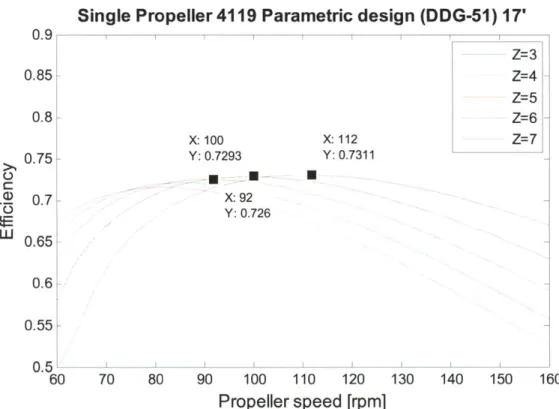
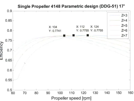
3.3.1 Single propeller (SP) param etric study ... 51
3.4 Final design...60
3.4.1 Single propeller final design ... 60
3.3.2 Contra-rotating propeller final design... 62
3.5 Off-design analysis for DDG-51... 65
3.5.1 Single propeller off design analysis ... 65
3.5.2 Contra-rotating propeller off design analysis... 66
3.5.3 SP and CRP efficiency com parison ... 74
Chapter 4 -Fuel consum ption com parison... 79
4.1 From hull resistance to required thrust pow er...80
4.2 From open w ater pow er to required thrust power ... 82
4.3 Propulsion efficiency chain...84
4.4 M atching the designed propellers to DDG-5 ... 85
4.4.1 M atching single propeller to DD G-51 load curve... 85
4.4.2 M atching CRP to DDG-51 load curve ... 88
4.5 Fuel Consum ption ... 90
4.5.1 From propeller thrust coefficient to required engine brake power... 90
4.5.2From engine brake power to fuel consum ption... ... 93
Chapter 5 - Prototype M anufacturing... 96
5.1 M odeling the propellers ... 97
5.1.1 Full scale propeller selection... 97
5.1.2 Sim ilitude analysis ... 98
5.2 Propeller design w ith Solid W orks ... ... ... 100
5.3 The prototypes production- FDM process ... 102
5.4 Experim ental set up... 104
5.4.1 N aval Academ y tow ing tank... 104
5.4.2 Test plan... 105
Chapter 6 - Sum m ery...106
6.1 Conclusions... 107
6.2 Recom m endation for Future W ork ... 108
References...111
A ppendix A-Circum ferential induced velocity...117
A. 1 Self-induced velocity ... 117
A .2 Circum ferential m ean velocities ... 118
A2.1 Axial interaction velocities: ... 118
A2.2 Tangential interaction velocities ... 119
Appendix B -M atlab codes ... 121
B.1 CRP_Analyzer.m ... 121
B.2 FuelConsum ption.m ... 133
B .3 Test Plan.m ... 138
A ppendix C - N aval propellers properties ... 141
List of Figures
Figure 1-1: Representation of the propeller blade as a lifting line, reproduced from (Kerwin and Hadler, 2 0 1 0 )...1 8
Figure 1-2: Propeller coordinate system and velocity notation, reproduced from (Kerwin and Hadler, 2 0 1 0 )...1 9
Figure 1-3 : Velocity and force diagram at a radial position on a lifting line, reproduced from (Epps,
2 0 10 b )...2 0 Figure 1-4: CRP velocities and forces diagram on one component of the set, reproduced from (Coney,
1 9 8 9 )... 2 7
Figure 3-1: DDG-51 total required thrust (Tsai,1994))... 49
Figure3-2: Parametric study using the blade chord distribution of US Navy propeller 4119...52
Figure 3-3: Parametric study using the blade chord distribution of US Navy propeller 4381...52
Figure 3-4: Parametric study using the blade chord distribution of US Navy propeller 4148...53
Figure 3-5 : Single propeller efficiency for a range of propeller diameters... 54
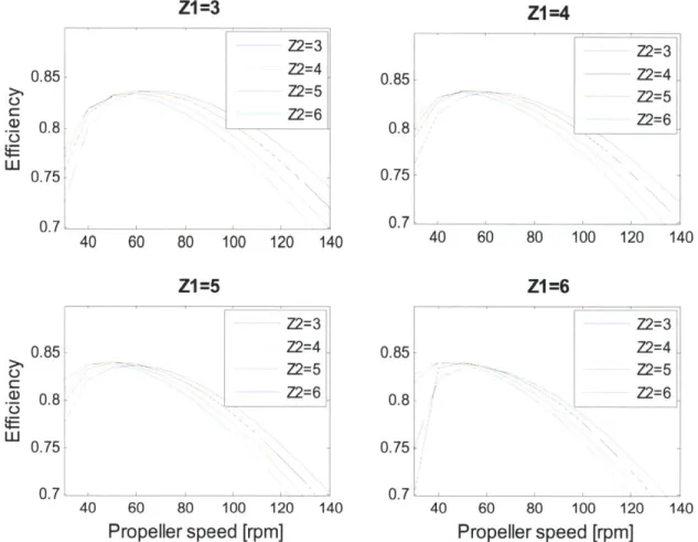
Figure 0-6: Contra-rotating propeller parametric study - range of propeller blades ... 56
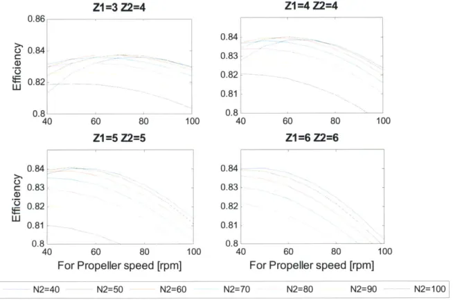
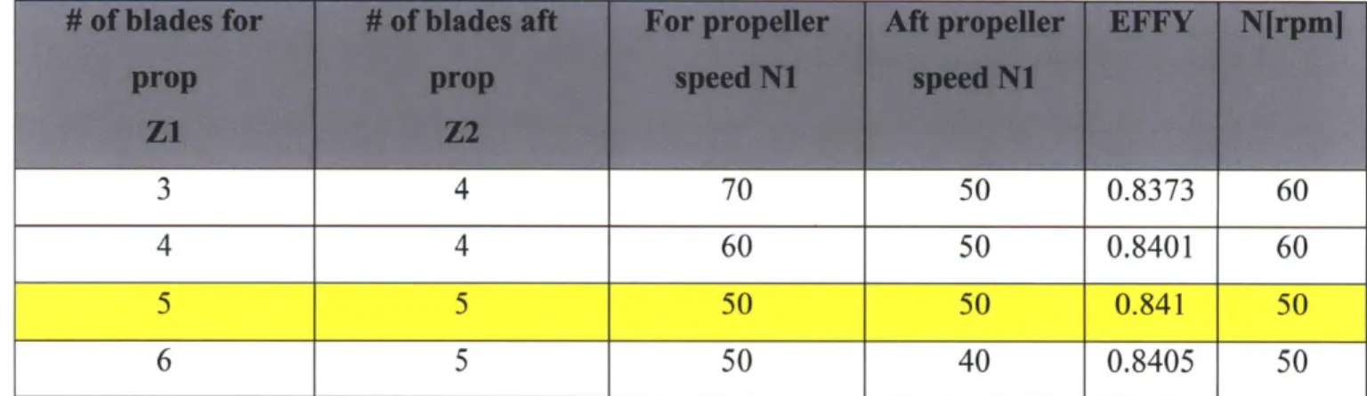
Figure 3-7: Contra-rotating propeller parametric study - range of propeller's speed...57
Figure 3-8: Axial separation param etric study... 59
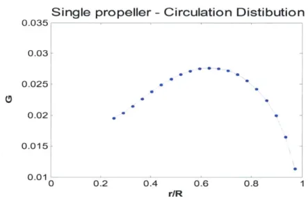
Figure 3-9: Non dim ensional circulation distribution ... 61
Figure 3-10: DDG-51 final Single propeller design cavitation map (for steady inflow speed)...61
Figure 3-11: Non dim ensional circulation distribution ... 63
Figure 3-12: Final contra-rotating propeller 3D im age ... 63
Figure 3-13: C RP cavitatio n m ap ... 64
Figure 3-14: Single propeller off design perform ance ... 65
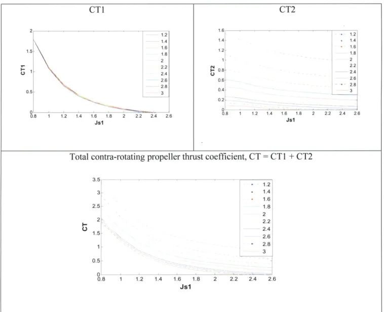
Figure 3-15: Contra-rotating propeller thrust coefficient, CT... 67
Figure 3-16: Evolution of the propeller thrust coefficient ... 68
Figure 3-17: CRP torque coefficient (CQ )... 69
Figure 3-18: Contra-rotating torque coefficient (KQ)... 70
Figure 3-19 : Total propeller thrust coefficient... 71
Figure 3-20 : Total propeller torque coefficient ... 71
Figure 3-21: CRP Hub drag coefficient ... 72
Figure 3-22 : CRP efficiency for different aft propeller advance ratios (Js2) curves...73
Figure 3-23: CRP m axim um off design efficiency curve... 75
Figure 3-24: CRP Maximum off design curve for same and different propeller speed ... 76
Figure 3-25: Single and Contra-rotating propellers efficiency comparison ... 77
Figure 3-26 : Single propeller and CRP on and off - design efficiencies with maximum curves...78
Figure 4-1 : DDG-51 Thrust coefficient vs. ship speed ... 86
Figure 4-2 : Single Propeller Thrust coefficient vs. advance ratio ... 87
Figure 4-3 : CRP Thrust coefficient vs. for propeller advanced coefficient ... 88
Figure 4-4: CRP thrust coefficient at advance ratio combinations which produce max efficiency ... 89
Figure 4-5 : CRP required interpolated torque coefficient ... 91
Figure 4-7 : DDG-51 actual operational profile data took from (Surko and Osborne, 2005)...93
Figure 4-8 : DDG-51 actual specific fuel consumption data took from (Tsai, 1994)... 94
Figure 4-9 : DDG-51 annually fuel consumption calculated for the designed SP and CR propellers...95
Figure 5-1: CRP1 Torque coefficient, the green line represent the equal torque coefficient ... 99
Figure 5-2: single and contra-rotating propeller (CRP1) geometry as produced by the Matlab code...100
Figure 5-3: CRP1 as designed by Solid w orks... 101
Figure 5-4: The electric m otor equipped w ith the CRP set...101
Figure 5-5: Picture of the CRP1 set connected to the electric motor at the preliminary tests ... 103
Figure 5-6: Picture of the CRP1 set connected to the electric motor at the preliminary tests ... 103
Figure 5-7: US Naval Academy 380 foot towing tank ... 98
List of Tables
Table 3-1: DDG-51 geometric parameters of the underwater hull... 48Table 3-2: DDG-51 Propeller parameters (Tsai,1994)... 48
Table 3-3 : DDG-51 design characteristics... 49
Table 3-4 : Propeller geometric restrictions... 50
Table 3-5 : 2D blade geom etry ... 50
Table 3-6: Single propeller parametric study summery... 53
Table 3-7 : Contra-rotating additional requirements ... 55
Table 3-8 : Contra-rotating propeller parametric study summery for a range of propeller blades56 Table 3-9 : Contra-rotating propeller parametric study summery for a range of propellers' speeds ... 5 8 Table 3-10 : Single propeller design specifications... 60
Table 3-11 : Final DDG-51 CRP specifications ... 62
Table 3-12: Design specification for SP and CRP... 74
Table 5-1: Propeller models main characteristics... 98
Introduction
The concept of contra rotating propellers is a very old one nearly as old as the invention of the screw propeller itself. However, the complex shafting and gearing associated with this propulsion system has prevented the wide use of this concept. Only relatively few modem applications are known.
The development of the electric propulsion in general and the podded propulsors in particular in the recent years, bring to mind of the naval architecture this type of propulsors .Contra rotating propulsion systems have the hydrodynamic advantages of recovering part of the slipstream rotational energy which would otherwise be lost to a conventional screw propeller system. The application of this type of propulsion becomes even more attractive with the increasing emphasis on the last years on fuel economy and the improvement of the propulsive efficiency. A design tool and a thorough study of the contra rotating propeller performance are in great demand.
OPENPROP is an open source propeller design and analysis code that has been in development since 2007 at MIT (Kimball and Epps, 2010). The theory contribution of this thesis is by adding another feature to this source with the implementation of the off design analysis for contra rotating propeller.
The history of contra-rotating propellers and the design theory behind the contra-rotating code are introduced in chapter one. Chapter two presents the CRP off design theory. Illustration of a contra-rotating design procedure for the DDG-51 ship class, using the off design code with the inclusive of a comparison of the two propulsors; single and contra rotating propeller are presented in chapter three. Once the efficiency superiority of the contra-rotating propeller over the conventional single propeller was studied in chapter three, the consequence with respect to the ship fuel consumption was investigated in chapter four. The propeller model design and manufacturing procedures for future experiments is described in chapter five. Conclusions and future work recommendation are presented in the last chapter of this thesis. All the supplementary calculations as well as the Matlab codes are shown in the appendices for a full completion of this work.
Chapter 1- Propeller Design Background
1.1 The history of marine propeller development
Along the marine ship design history people have always looked for new technologies to improve the ship propulsion efficiency. Whenever presenting any new novel propeller technology, the history of the predecessor evolution types is important to be introduced as well. Therefore, despite the essence of this work is the contra-rotating propeller design methodology, the development of the marine propeller over the history which leads to the contra-rotating propeller idea, will introduced in this chapter.
1.1.1 Screw propeller
The concept of screw propeller dates back to the 950 BC; the Egyptians used a screw-like device for irrigation purposes. Archimedes (287-212 BC) and later Leonardo da Vinci (1452-1519) created and drew water screws devices for pumping purposes (Taggart, 1969). However, only at the mid-17th century, the development of steam engines contributed to effective use of screw propellers and only at that time the concept of screw propeller transformed to marine propeller. Nevertheless, the screw propeller was still considered as a second mover to the paddle wheel at this time. The acknowledgment for the invention of the modem style propeller goes to Smith and Eriksson who acquired patents in 1836 for screw propellers (John Ericson RINA affairs, 2004), marking the start of its contemporary development. Eriksson's propeller design took advantage of benefits of the bladed wheel. The final step to what is now recognizable as a screw propeller was made by George Rennie's conoidal screw, Rennie combined the ideas of increased pitch, multiple blades, and minimum convolutions in what he called a Conoidal propeller, patented in 1840 (Taggart,1969). Screw propellers installed in the late of the 19th century lacked sophistication, but their performance exceeded all other devices conceived up to that time. During 1880 to 1970 Basic shape of propellers remained unchanged. Ever since, marine propeller technology has made some advancements toward greater efficiency, more reliable design, better performance, improved materials, and cavitation resistance. Marine engineers are still looking for new developments of unconventional propellers to improve the propeller efficiency and consequently the total ship fuel consumption. Among these new
developments count up the controllable pitch propeller (CPP), Skewback propeller, ducted propeller, Cycloidal propellers, water jet propulsion, and podded and Azimuth podded propulsion systems.
1.1.2 Contra-rotating propeller
The concept of having two consecutive propellers behind each other, rotating in different directions is not new. In fact, this concept is as old as the screw propeller itself, as John Ericsson's patent of 1836 included single, twin, as well as contra-rotating propellers (John Ericson RINA affairs, 2004).Although the high efficiency obtained with contra-rotating propellers has long been known, until fairly recently material technology and the need for long concentric shafts running in different directions, made the concept both technically and economically unfeasible. However, in the mid 1980's contra-rotating propellers were successfully introduced in azimuth thrusters for, utilizing the short propeller shaft and bevel gear. In the late 1980's, a distinct concept has made its way into the marine world. This new concept is referred to as podded propulsor and is distinguished from the original thruster in that its prime mover is an electric motor, situated in the hub, directly driving the propeller. The idea of placing the electric propulsion motor inside a submerged azimuthing propulsor arose by Kvaerner Masa-Yards, together with ABB Industry. Over the last decade since, podded propulsors have become more and more important, particularly on cruise liners.
In the new millennium, efforts have been concentrated on development of a novel propulsion plant using the pod unit; it has been found that the "CRP-POD propulsion system," combining the conventional propeller propulsion system with pod propulsion, is sufficiently economic and competitive in general merchant ships. The combined high efficiency of CRP and the excellent maneuverability of podded propulsors make the hybrid CRP system extremely attractive.
The concept of contra-rotating propellers can be found also in aeronautics industry, Contra-rotating aircraft propellers came into service at the end of WW II. This configuration offered a number of advantages including lower asymmetrical torque, higher efficiency, and smaller propeller disk (allowing shorter landing gear), (Carlton, 2008). But the complexity caused by the gearing mechanisms and the expensive maintenance costs resulted in the delay of contra-rotating propeller entering into service. Other fields the contra-rotating propellers are used are in the wind turbine field and in tide turbine for ocean energy utilization.
1.2 Propeller design methods developments
From the beginning of the screw propeller concept till the 19th century(the Industrial
Revolution) the propeller design were based upon trial and errors ;i.e., the propeller designer produced a baseline propeller while utilizing its geometry to detect the performances changes until the best results (from their point of view) are achieved. Only at 1865, with the introduction of the Momentum theory by Rankine, the propeller design methods began to evolve.
Momentum theory, Rankine (1865-1887): This theory is based on the axial motion of the water passing through a propeller disc. The propeller thrust can be estimated by calculating the change in the waters momentum across the two faces of the disk. This theory did not concern with the propeller geometry, since the propeller is replaced by an actuator disk. Hence, this method is not useful for blade design purposes. His result, however, leads to some general conclusions about propeller actions, in particular the optimum efficiency which can be delivered by a screw propeller, named as the "Actuator disk efficiency", (Rankine, 1865).
Blade element theory, Froude (1878): In contrast to Rankin's theory, Froude developed a method which takes into account the propeller blade geometry (Froude, 1889). In his model, the propeller blade was divided up to a large number of elements; each element can be regarded as an aerofoil subject to an incident velocity. This model allows the propeller thrust and torque to be calculated provided the appropriate values of the aerofoil drag and lift coefficients are known. Although Froude's work failed to predict the propeller performance accurately, since the blade elements drag and lift coefficient were hard to find, it contained the basic principles upon modern theory is founded (Carlton,2008).
Propeller theoretical development (1900-1960): Lanchester and Prandtl (1919) were the first who put forward the concept that the lift on a wing was due to the development of circulation around the blade elements and that a system of trailing free vortices shed from each section. The application of this theory was the understanding of the axial and tangential velocities induced by the free vortices on the blade element. Bets (1919) and followed by Lerbs (1952) established conditions for formatting the optimum circulation along the propeller blade. Lerbs introduced the lifting line method which can produce a great prediction for the moderately loaded propeller performance working in an inviscid flow At these time many lifting line procedures were formed to numerically calculate the propeller performance also for light
and heavy loaded base on different assumptions, such as Burrill (1944), and Morgan and Eckhardt (1955).The lifting line methods mostly used for preliminary design since its highly computational efficient. For a detail design and analysis, however, more accurate methods were developed.
Lifting surface model (1960-1995): In this model the blade is replaced by an infinitely thin surface which take the form of the blade camber line and upon which a distribution of vorticity is place in both spanwise and chordwise directions. Later, the sectional thicknesses could be modeled by adding a distribution of sources and sinks in the chordwise direction. In the early 1960s many lifting surface procedures made their appearance mainly due to the various computational capabilities that became available at that time. Pien (1960) is generally credited with producing the first lifting surface theories. The vortex lattice method, Kerwin and Lee (1978) is a subclass of the lifting surface method. In this approach the continuous circulation distribution (as well as the source and sinks distribution) is replaced with discrete values along the blade (or chordwise).This method found to be mostly efficient with respect of the propeller performance predictions. The basic lifting surface, however, with respect to computational efforts this method is not satisfactory efficient. Therefore, is mostly used for detail design propeller and performance analysis.
Boundary element methods (1980: recent years): This method was developed in the recent years to overcome two problems with the lifting surface models. First, is the occurrence of local errors nearby the leading edge, and the second is the errors which occur near the hub where the blades are closely spaced and relatively thick. In this method the surfaces of the propeller blades and the hub are approximate by a number of small hyprboloidal quadrilateral panels having constant source and doublet distribution. The trailing sheet is also represented by the same panel geometry. The strength of the source and doublet values are determined by solving the boundary problem at each control point which are located at each panel. Using methods of this type, good correlation between theoretical and experimental results for pressure distribution along the blade and propeller performances has been achieved.
Computational Fluid Dynamics (21st century): In the last decade, considerable advances have been made in the application of computational fluid dynamics to the analysis and design of marine propellers. A number of approaches for modeling the flow around the propeller plane have been developed. These approaches are the Reynolds Averaged Navier-Stokes (RANS) method, Large Eddy Simulation (LES), and direct numerical simulations (DNS).However, the
application of many of these methods is limited by the amount of computational effort required to derive a solution. The RANS codes were found to be the most efficient with regarded the computational effort. For this reason, these methods are currently used for research purposes rather than a practical propeller design. The usage of these method will increased in the following years with the developments of fast computers (the computer processors speeds double itself, in general, every two years)
1.3 Single propeller lifting line theory
What follows is a summary of propeller lifting line theory; following the formulations of Kerwin and Hadler (2010).The lifting line which used in marine propeller is by representing the Z number of blades by straight, radial, lifting lines. The bound vorticity distribution along each of the blade radial chords (,,x , is replaced by a concentrate single circulation F()
.
Since all blades are equal loading and consequently have the same circulation distribution in circumferentially uniform flow, we can select one blade (or lifting line) and designate it as the key blade. The blade geometry: camber, pitch, chord, thickness etc., are represented by this radial circulation distribution. The lifting lines start at the propeller hub rhub and extended to the maximum propeller radius, R. Figure 1-1 demonstrates the propeller blades as a lifting line.Y Y
Since the inflow is unsteady relative to the ship fixed coordinate system the chosen coordinate system is cylindrical (x, r, 0) with the x axis coincident with the axis of rotation of the propeller.
The origin of the coordinate is in the plane of the propeller, which serves as the reference point for all axial dimensions of the propeller blade surfaces. The radial coordinate is denoted
by 'r', and the angular coordinate by '0', which is measured in a clockwise (right-handed)
sense when looking downstream with 0 = 0 being at 12 o'clock. In most cases we would find that the variation in inflow velocity would be slight in the x direction, it is therefore customary to assume that the inflow field is independent of x, and that the inflow stream tubes are therefore cylindrical. To be consistent with this assumption, conservation of mass then requires that the circumferential mean radial inflow velocity be considered to be zero. However, tangential inflow velocities may be present. The coordinate system and velocity notation are describes in figure 1-2. Ur Ua .0Ut
z
0')LQI
X
U--The velocities and forces diagram at a radial lifting line point are described in figure 1-3.
F,
lea
as drawn
t <
0
F V a ' VO
Va
Figure 1-3 :Velocity and force diagram at a radial position on a lifting line, reproduced from (Epps, 2010b).
VA and VT are the axial and tangential inflows velocities, respectively. r is the lifting line radial location, wr is the propeller rotational speed, u*,u* are the axial and tangential induced velocities, respectively.
#3
is the hydrodynamic pitch angle ,and 8 is the same angle when the propeller induced velocities are not taking into account. O, is the geometric pitch angle , a isthe angle of attack ,and V * is the total relative speed which is calculated by the next equation,
V* = J(V+u ± )2 +(w r+V, +u*)2
and its orientation with respect to the plane of rotation -the hydrodynamic pitch angle is,
8
= arcta a +a]w r +V +u,
(1. 1)
Expression of the inviscid force (lift) acting on a vortex locates at radius r, can be calculated using the local Kutta-Joukowski's law:
F, = pV*F (1.3)
and is directed at right angle to the total relative velocity (V*).
The effect of the viscous drag force on the radial section can be determined by 2D experimental data or by theoretical means of the two dimensional drag coefficients. The radial viscous force can be expressed as:
F,
=p )V*CD '(1.4)where c is the radial chord length and CD is the 2D drag coefficient. This force acts with direction parallel to V*.
To produce the total propeller thrust and torques, the lift and viscous forces are parted into two forces; axial (thrust) and tangential torque). The radial forces are then integrated along the blade (from the hub radius to the max blade radius), and multiple with the number of blades Z. The total thrust (T) and torque (Q) will then be:
T = pZ [V*Fcos
I
(V*)2cCD sin8]dr (1.5)Rhub
Q=
pZ [V*Fsin/,i + (V*)2cCDc i]dr (1.6)Rhub
where V* -cos
p,
is the tangential velocity equal to w r + V, + u* ,and V* -sinp,
is the axial velocity equal to V, + u.After formulating the required equations for computing the propeller thrust and torque, the propeller efficiency is then can calculated. However, the circulation distribution and the radial induced velocities are still unknown. The following sections will introduce the Vortex lattice
model theory, which estimates a solution for the induced velocities and then, the optimum circulation distribution methods will be presented. However, because these theories are not the main subject of this work and they are well studied and presented in many works since the established of the lifting line theory (e.g. Kerwin and Hadler, 2010; Epps, 2010b) only a general review of the basic concepts, which are important to understand the contra-rotating propeller design method, will be introduced.
1.3.1 Vortex lattice model
In this model, each lifting line is divided to M panels of length dr . The induced velocities are calculated at control points located at the mid of each panel. The continuous bound circulation distribution is replaced with a discrete distribution lengthwise each of the lifting lines panels with strength ,(m, located at radius r(m). The helical free vortex sheet is replaced with a concentrated
helix vortices shed from each panel boundary. Therefore, the discrete circulation distribution can be thought as a set of vortex horseshoes, each assembles one bound vortex segment with two free trailing helix vortices. The strength of each free trailing vortices is equal to the strength difference of two adjacent bound vortex along the blade F(,,, - F(.)
The velocity induced from this vortices system are computed with the asymptotic formula developed by Wrench (1957), appendix A. l.The total induced velocities at each control point is the summation of the velocity induced from an individual horseshoe vortex at that point,
M Ua(n) - ' (m) Ua(n,m) (1.7) m=1 M u,(n) (m) t(n,m)(.8 m=1
where u u* are axial and tangential total induced velocities at control point n, respectively.
F ,is the strength of horseshoe vortex locate at radius rv(m). U t, are the axial and
tangential influence functions; velocity induced by a unit strength horseshoe vortex surrounding the control point at r(,) .
The integrations of equations 1.5 and 1.6 under the discrete form are replaced in by summations over the number of panels (M):
T =pZ
{
[V , +wr,) +u, ] -. ) Ar -V* ,[V, +* D(m)(1.9) =1 tt)* ( in 2 (n) IV(.n) + Ua(i) ]C(, CD m rQ=PZZ { [Va(,) +u a,()] [1(,,l)r(,,)Ar + I V , , +wr ,0+*, ]c ,,)CDim)r)Ar
}
(1.10)rn=i 2 Mn)~(n w +u U*~)I~)C~)rM
All characteristics at equations 1.9, 1.10 are computed at control point located at radius r m).
These equations can now be solved if the discrete circulation distribution is known.
1.3.2 Optimum circulation
To design the most efficient propeller for a specified design point, an optimum circulation distribution method should apply. After successfully computing this distribution, the other essential propeller characteristics could analyze. During the design process, however, the circulation distribution might depart from its optimum while other considerations, such as; inception of tip vortex cavitation, are taking into account.
Betz (1919) developed an optimum condition for propeller in uniform flow based on the variational principles and Munks theorem; which states that the total force on a lifting line is unchanged if an element of bound vorticity is displaced in the streamwise direction. His result suggested that the ultimate forms of the vortices far downstream for an optimum circulation distribution are true helices and is expressed as:
tan
p.~
tanA = const (1.11)
tan/#
The unknown constant is a function of the required propeller thrust. Lerbs (1952) expanded Betz criteria to non-uniform axial flow:
tan/i = const - 1- w
(1.12)
tan
p(
here, Wx(r) is the radial wake fraction and the constant is a function of the propeller thrust.
Different procedure for calculating the optimum circulation distribution is suggested by Kerwin, Coney and Hsin (1986). In their procedure the optimum distribution is achieved by minimizing the propeller torque (equ.1.10) subjected to a constraint of a given thrust Tr. The required auxiliary function can, then, be formulated:
H = Q-A(T-T) (1.13)
A is the Lagrange multiplier. When partial differentiate this function with respect to the unknowns circulation F(m) and the Lagrange multiplier and set to equal zero, the solution will provide the desirable optimum circulation distribution as well as the Lagrange multiplier.
1.3.3 Propeller geometry
Once computing the optimum circulation distribution, the required radial lift coefficient is calculated,
CL( ) (1.14)
CL(i) is the required radial lift coefficient. The problem now is diminished to find a suitable
blade section geometry which provides the required lift coefficient. The lifting theory, by itself, does not provide any method to determine the lift generated by a particular foil shape, since the details of the flow over the actual surface are completely lost in the idealization of the lifting line. The NACA serious is, hence, should be introduced.
A series of foils geometry were developed and tested by the NACA in the 30's and 40's, Abbott & Von Doenhoff (1959) tabulated all this data, and is known as the 'a' series, where the "a" denotes the fraction of the chord over which the circulation is constant. In this source many foils geometry (meanlines and thicknesses) were examined by a set of experiments and the resulted flow data were tabulated, amongst is the foil ideal lift coefficient and angle of attack. All it is necessary to complete the propeller design is to linearly scale the required lift coefficient with the chosen foil's one ,and do the same for the angle of attack to find the required radial section geometry; meanline and orientation. One foil type, the NACA meanline a=0.8 and the NACA 65A (TBM) basic thickness form was widely adopted by propeller designers for marine propeller and is also used in this work.
In summary, the first step of the lifting line linearization process was to find the required radial lift coefficients by computing the optimum circulation distribution and the velocities induced by these circulations on the lifting line. Then, the 3D problem is diminished by choosing a proper 2D foil geometry which can provide the required lift by linearly scale its characteristics
with the desired lift coefficient. These characteristics; the ideal angle of attack and the foil geometry are the base for the propeller design.
1.4 Lifting line method for CRP
The first lifting line design method for two coaxial open propellers separated apart with some distance and rotate in different directions is refer to Lerbs (1955).His contra-rotating design scheme was an extension of the single propeller lifting line with the inclusive of the interaction velocities induced by each propeller on the other. Lerbs first modeled an "equivalent" propeller while assuming no axial separation between components, compute the required characteristics of this propeller while considering the desirable thrust to be one half of the total thrust .Then, he decomposed the equivalent propeller to two separate ones. In his work the two propellers have the same number of blades. Morgan (1960) derived again Lerbs' theorem for a free running and a wake adopted inflow with the extension of any combination of number of blades. Morgan and Wrench (1965) rederived the differential equation for the equivalent circulation distribution of the CRP set, and most important derived accurate equations to calculate the interactive induced velocities.
Contrary to Morgan et al (1965) who decoupled the CR propellers to two different units and then designed the required characteristics by coupling two single propellers code in an iterative way, Kerwin,Coney and Hsin (1986) considered the CRP set as an integrated unit. This method was the extension of the variational scheme of the single propeller. According to them, the lifting line method for designing a contra-rotating propeller takes into account the two propellers as an integrated propulsive unit .Next; an iterative procedure is established to calculate the optimum circulation distribution at each propeller. Laskos (2010) integrated both of these methods, referring to them methods as "coupled" and "uncoupled". A major distinguish between the two is that in the "uncoupled" method, two separate sets of equations are established and then are optimized. The parameters which bond the two sets of equations, unlike from being two separated single propellers, is the consideration of the mutual velocities induced by each propeller on the other. In the "coupled" method, on the other hand, one complete set of equations is formulated and then is optimized. One of the advantages of the last method is the ability to design a multi component propeller.
The next sections will introduce the system of equations formulating the self and interaction velocities induced by each propeller component. The optimization process of the circulation distribution over each propeller lifting line will introduce as well.
In this work, the "coupled" design procedure of Kerwin, Coney, and Hsin (1986), as implemented by Laskos (2010) is used.
1.4.1 Self and mutual Induced Velocities
As mentioned in section 1.3.1, the discrete horseshoe vortex surrounding each of the m'th control point on the lifting line, consist one segment of bound vortex and two free trailing vortices shed from the panel boundary. For straight, radial, lifting lines with equal angular spacing and identical loading, the self-induced velocity at each propeller is only due to the free trailing vortices. For a purely helical wake geometry, these velocities can calculated using the
asymptotic formulas developed by Wrench (1957) as same as for the single propeller case.
The mutual induced velocities on each of the lifting lines component's plane are the velocity induced by the other components' lifting lines vortices. Contrary to the self-induced velocity, the interaction velocities come from both; the bound and free vortex sheet. It can be seen from a simple geometric relationship that the circumferential mean interaction velocities induced by the bound vortices contribute only in the tangential direction. The circumferential mean interaction velocities induced by the free vortices, on the other hand, consist of axial, tangential and radial velocities. For calculating the steady forces delivered by each component the time-averaged interaction velocities are those of interest.
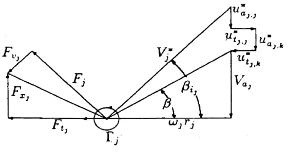
The contra-rotating velocity and forces diagram on one component of the CRP set is presented in figure 1-4.
Lj -j
F
V
-FF
FF
Figure 1-4: CRP velocities and forces diagram on one component of the set, reproduced from (Coney, 1989). * * here,
j
indicates one of the components (j = 1,2 ),k is another component indicator. Ua , Uajk* *
are axial self and interaction induced velocity on component
jU
U 1 , k are the tangential selfand induced velocities on component
j,
respectively.The radial interaction velocity component induced by each component is not of interest since it is not contribute to the total forces acting on the blade. Moreover, a basic assumption of the CRP code is that the slipstream is not contract, thus, the radial velocity is set to zero (by default).
Hsin (1987) compared several of methods to compute the circumferential mean interaction velocities and he found that the method developed by Hough and Ordway (1965) was the most computationally efficient way to do so. For the part due to the free trailing vorticity, the tangential induced velocities by the bound vorticity can be computed directly from the circulation conservation application of Kelvins theorem. The set of equation formulating both the free and bound induced interaction velocity are introduced in Appendix A.
1.4.2 Optimum CRP circulation distribution process
As already mentioned, the CRP code employs the described "coupled" method. In this approach one set of differential equation is formulated and is solve simultaneously to produce the loading and the circulation distribution at each component of the unit. Following Kerwin, Coney, and Hsin (1986) ,the goal is to find the discrete circulation strength values
F, . .F PIF 2 - - Fu2 .that minimizes the total power absorbed by the propeller unit ;
p = w1Q1 + w2Q2,when subjected to two constraints; the propeller needs to deliver thrust Tr for a specified moment ratio absorbed by each propeller q = Q1/ Q2 .
The auxiliary function consists the three conditions can now be formed:
H = (wQ + w2Q) + AT(TI + T2 - T,)+A,, (qQ -
Q2)
(1.15) From now and on, subscript "1" denotes to the forward propeller and "2" refer the aft propeller.Mi and M2 are the number of panels dividing the key lifting line on each component.T1,T2are the thrust carried by each component, respectively.
The thrust and moment forces acting on each component are the sum of the inviscid and the viscous forces acting on all control points along the propeller lifting lines.
M1 *
T =pZ { [V (,) + wr() +u*,,)] Fj(,)Ar. - - V+un) [Va + Uan]*] Cn
T np = { [ ± w 2c (n i n) c Dj(n) ]
}
(1.16)
M
Q
p Z{
[ V a i ( n ) + u *J f l ] .-] ( f l r J , A r + * + w r + u+ uF] ci( n C D ( j ) ( j )A) j 1 '7 \n=1p+Y{ Vi(nl) IVY(f) + jir(n) + U(n) 1CfIC~ nr~nA,-J l.l7)
here, (n) represents, the control point 'n' at component
j
,were j=1,2.The axial and tangential velocities induced on a given control points are the sum of the self and interaction velocities induced from each of the horseshoe vortex on the lifting lines can be written as: K M u a (n) =::F () uaj (n) (1.18) k=1 m=1 K M u* (n)= I k(M U * (n) (1.19) k-i rn-k=1 m=1
j,k= 1,2
are the axial and tangential velocities induced at control point 'n' of component
j
by horseshoe vortex of unit strength surrounding control point m of component k.Fk(m) is the horseshoe vortex strength surrounding control point 'in' of component k. Whenever j=k, the velocity is the self-induced velocity, otherwise it is the interaction induced velocities.
After determining all the constituents in the auxiliary function with respect to the discrete circulation strengths F,, the optimum circulation values can now be computed. While computing a partial derivative of the auxiliary function with respect to the unknown circulation and the unknown Lagrange multipliers ATA. and equal set to zero, the results provide the required optimum circulation values at each propeller. The partial derivative can be written as follows:
=0= WI
ag,
i- (i)
+Q
2+
8F
1(i)
+i 2 ___1 ___2 AT,[ + ] + Q[_ Q ]Qafj (i) 80j (i) NJy (i) -aFj (i)
aQ
(w, + qaF)
(
aryj (i)
- a 2 +07(i)
AT
aT
,[ 1 + 2 ]aF
1(i)
8F
1(i)(1.20)
(1.21)
(1.22)
O-O=T
+T-= 0 = 1 T 2 - T r
aH_
H= 0 = qQ, -Q
2This is a system of M1+M2+2 nonlinear equations, and the same number of unknowns;M1 circulation values on the forward key lifting line, M2 circulation values on the aft key lifting line,
and two unknown Lagrange multipliers. Kerwin (1986) sets-up an iterative procedure to solve * * this nonlinear problem. The Lagrange multipliers ATr,A% and the induced velocities Ua ,U, are frozen and then updated at each of the iteration set. This procedure found to converge rapidly when the initial values for the induced velocities and the multiplier A Q are set to zero and the multiplier AT is set to -1.This process is implemented in the CRP analysis code by Laskos (2010).
aH
aF,(i)
Chapter 2 - Off Design Analysis
2.1 Chapter introduction
The general propeller design procedure generates the optimum propeller characteristics for the required ship on design demands which commonly restricted by several constraints such as; hull geometry, speed engine etc. The output of the optimization process is the necessitated radial circulation distribution over the blade span (F) corresponded to the radial hydrodynamic pitch angle (i), at each propeller. This procedure is generally suitable for both; single and contra-rotating propellers and will describe in the following chapters. Once the required circulation distribution was computed, the required sectional lift coefficient (CLo) is calculated using equation 1.14.Based on this required lift coefficient and a 2D foil shape parameters /c,5
},
a determination of the blade geometry parameters; required sectional camber ratio (f.), and the required radial ideal angle of attack (a,) which produces the desired characteristics, is linearlyscale to produce the propeller blade required geometry.
The above procedure demonstrates the design process for single and contra-rotating propeller. In order to analyze the propeller performances at off design state an additional analysis is required. The subject of this chapter is to establish a numeric procedure to analyses the contra-rotating off design states. This procedure is an extension of the single propeller off design analysis Epps (2010).
2.2
CRP off design analysis -theory
From this point until the end of this chapter, the on design characteristics will be added with the following subscription: CLO, aO,
fl
0,
CDO, while the off design unknowns will remain without any particular subscription: CL, a, ,CD.In addition, subscripts k=1,2 are correspond to the forward and aft propeller, respectively.After the propeller geometry was defined at the design process, a method to determine the contra-rotating propeller off design states performances is required to be established. The objective is to comprehend the propeller performance in a range of off design states (advance ratios); various propeller rotational speeds with different ship speeds.
The basic concept to cope with the off design problem is to find a method to solve a system of nonlinear equations with the same number of unknowns. The method described herein follows that of the single propeller analysis developed by Epps (2010a). The off design (OD) operating state is defined by the propellers advance coefficient,
Vs cVs
JslOD - Wl)T~s (2.1)
n10DDI
wiODRIJs = Vs _ ;TVs
n2ODD 2 W2ODR2 (2.2)
where Js OD,JS20D are the advance coefficients; Vs is the ship speed [m/s]; n ,n are the
propellers rotation speed [rps] ;w ,W 20 are the rotation rate[1/rad]; and DI,D 2 are the
propellers diameter [in].
For a given advance coefficient, the hydrodynamics unknowns are,
a*,a C G1,u* ,u,*i ut'*1u for the forward propeller,
V2*
a2,
CL2, G2,u*2,u,2 9 aii2 ,i iUit22,il'n1} for the aft propeller.The unknown are vectors of size [1, Mp], where Mp is the number of control points lengthwise the blade.
Contradicting to the single propeller off design state, the CRP off design state is depended by the rotation rates of both propellers; fore and aft, which makes the process to be more complicated.
2.2.1 The system of nonlinear equations
Before continuing, an equations for determine the angles of attack a,a2 and the lift coefficient CLJ, CL2 are required. The other equations which complete the system of equations
were already introduced in chapter two for the on-design analysis.
To achieve a shock free at the leading edge, the angle of attack at the design state is forced to be the ideal angle of attack, which is straightforwardly computed from the 2D foil shape. At the off design states, on the other hand, the radial angle of attack is not the ideal one, therefore, additional equations are required. Nevertheless, after the propeller geometry was found, the radial pitch angle (O, ) is fixed, hence the radial pitch angle at the off design state is the same as at on design state;
Op(k) ~ +aio(k) ajk) Ak) + aQk)
and the net angle of attack: Aa(k) a(k) -a (k) -pO(k) - p (k) (2.3)
The 2D section lift and drag coefficient are given in closed form by equations,
~ ±dCLk dC
CL(k) LOC)(k) da) Aa(k) - dL(k) (A ) - aSTALL) F(Aa ) - AaSTALL) ±
da k) da(k)
dC L(2.4)
+ (-k) a(k) -AaSTALL -F(-Aa(k) - AaSTALL
da k)
CDl CDOk)± A(Aa(k) -AaSTALL )F(Aa(k) - Aa STALL ) ±
+ A(-Aa(k) - AaSTALL )F(-Aa(k) - AaSTALL)- 2A(- AaSTALL )F(- AaSTALL) (2.5)
Where, A a(k) = a(k) - aI(k) [rad] is the net angle of attack, AaSTALL = 80 = 8. [rad] is the stall 180
angle; Fx) = arctan(Bx) +
±
is the auxiliary function; B = 20 is the stall sharpness parameter;2
2-C dC
A D01,2 is the drag coefficient post stall slope ;and the lift curve slope a,2 =2r - AaSTALL
2
This model is also used for the single propeller off design analysis at OPENPROP (Epps 2010b).The drag coefficient is not required for solving the system ,but it will be valuable when introducing the calculations of the off design forces.
Another set of equations which join all the other unknowns are not unique to the off design analysis, and were also used to find the optimum dimensionless circulation distribution, and to determine the propellers geometry at the design state. At that procedure the optimum circulation distribution (G,C 2) was first optimized and then the lift coefficient was computed through
equations 1.14. In the off design analysis, on the other hand, the lift coefficient is computed first using equation 2.4 afterwards the circulation is computed,
2CLk_ CL(k) k )C(k)
CL (k)c(k) (k
the relative velocity,
VM= (V +u(k))2
( OD(k) r + t Ut(k) 2
and the hydrodynamic pitch angle,
V +u*
p(k)
=arctan( " " ) (2.8)OD(k) r t t(k)
where, V *is the relative velocity; Va is the speed of advance, which in this work is equal to the ship speed; V is the transverse inflow speed; uk is the axial induced velocity at the fore and aft propellers; Ut*k) is the tangential induced velocity; and
p,
is the hydrodynamic pitch angle.The induced velocities at each propeller are the sum of the self and interaction induced velocities, the equations for calculating these induced velocities are described in chapter one, equations 1.181 and 1.19.
Up to now, the unknown and the system of equation for the off design states were introduced, in the next paragraph the numerical method for solving this nonlinear system will be presented.
2.2.2 Newton solver method
For a linear system of equations numerous analytical and direct procedures for solving the system are accessible in the literature, such as; the Newton's method, the bisection method, and the Jacobi iteration.
In this thesis the Newton's method was selected to be used for solving the off design states. This method can often converge remarkably quickly especially if the initial guess is sufficiently near the desired root. Newton's method can fail to converge with little warning so a smart initial guess is very important.
The idea of the method is as follows:
For a set of n nonlinear equations with n unknown,
fl..X1,I
X21 X3"
... Xf2..1..X21.X3--...Xn)
F(X)=
f 3(xix 2x3. -. ) =0fn
(xI,x 2,X3. .Xn)A linearization of the system, using the Taylor series expanded, can be done with the following conditions; if f is differentiable at the iterations guess (i) and x is near i then,
Df( 8(i)
a
8(k)f(x)~f (x -xi)+ (x2-x2)+ . + (xn - xn)
x2 n
and, in a vector form,
f(x)~
f(i)
+ J(k)(x - i) =f(k)
+ J(Xi)dxwhere f(x) is called the residual vector, and the derivative matrix (or Jacobian matrix) J(i) evaluated at 2 is defined as follow,
8f1(i) Of1(k) f;(i) xl 8x2 8xn af2(^) Of2(i) Of2(^) J(i)= Ox1 x2 8xn C'fn( 'fn(i af, ( ) Ox Ox2 Oxn
In order to derive the residual vector to zero the desired change in the state vector is found by solving,
f(i)+ J(k)dx = 0
dx=-J (Of( )
and continuing , the next guess for the next iteration is,
x* =+dx
X* is the new guess ,while i is the current guess. The new guess is installed back to the system of equation and the procedure is repeated until convergence.
2.2.3 Implementation of the Newton's solver
2.2.3.1 Final configurationThis paragraph demonstrate the implementation of the Newton's solver to find the off design states; solving the system of the off design nonlinear equations. Deciding which equations are added to the Newton's solver and which are left out is a very challenges task. Several Newton solver configurations were examined, in a manner of computer time consumption and a convergence of the system. A discussion of the options which were not integrated in the solver will be follow after introducing the final set up.
Since the system of equations are coupled through the parameters
{
pil,
iT1, Ua~t i1, 1 I andx = { V*,ai,CLl, G1, u*ju*,V, a2, CL, G2,u 2,u 2
},
andy = jii*2, 9a12 tI 1 'Ut12 5A #a1 i2 Ia22 * -* 22,*
During each iteration vector state x is updated at each control point (every unknown is actually a vector of M, control points), using the Newton solver method .With the updated x and equations: 1.18 and 1.19 vector y is then updated. A convergence test is then calculated, and if necessary, the procedure is repeated until convergence of the system.
The final residual vector consist the following equations:
V*
-I(V, +u*,) 2 +(wlODr t U 2 1a - ilO 1'lj CLI L1(al) 1 17-- CLIV*c1 Liii1 2 M1 M2 1l(m) I 1(j) all(mj) 2(j) al2(m j) M1 M2 tl(m) I 1(j) tl(n,j) 2(j) t12(mj) R == =V2* (Va +Ua 2)2 (W20Dr +t u%)
2
a2 a2ideal -(A20 18 2 - a2 -i 2O I2)
Co-C
CL2 - L2(a 2) 1. 2 L2V2 2 2 M1 M2a2(m) F2(j)i ai2 2(m,j) ± 1 () a21(m,j)
j=1 m=1
M1 M2
U r F(JU;+( I F i
t2(m) 2(j) t22(m,j) 1(j) t21(m,j)
_m=1 m=1 - 12*1
where, each of the unknowns is evaluated at the rc(m) control point, for each propeller; assuming both propellers have an equal number of panels (control points). This set up of the residual vector found to be the most efficient vector to lead the system to a finite solution. In order to drive the residual vector to zero, the desired change in the state vector dxm is found by solving the matrix equation:
Rm + Jdxm =0
where the Jacobian matrix, as was mentioned in the previous paragraphs, is the derivatives of each unknowns with respect to the unknowns others in the matrix.
J = 'R()
This matrix is complicated since all the variables in vector x are dependent to each other, and some are also dependent threw the other unknowns (vector y ); which were not included in the residual vector. The way to put together this matrix is by using the chain rule derivatives for two unknowns in the residual vector that are dependent by other unknowns which are not included in the residual vector. For all the others, the direct derivatives are computed.
Re. RaR ORc 8RG aRu*, aRu* BR,; 8R aRcL aRG2 DRua2 RURu2
_= - -- 1 (i=1...12)
t 1V, 1C G, a u * aCL 2 aG 2 a*2 ut*2
J
R - . ya+Ua* (1,5 al a U 1 2 ( OD1 cl t 2 aR .D1 cl t t1 (1,6) *1 j( ± 2 ±( OD cl±2
BRa 8Ra
p
8Ra 8pl atan(fi1) 1(25 Bu p u p tnp) B* +tan2 ,il) ODr' cl V t
au8ic, l - a*, '98i ~tfl\l ff* t +U ±V l
BRa BR ap_ aRa all 8tan(il1) 1 -tan(pJ 1)
au1 a,8, cu~ a,8lA oan ,, ±anp,61,, tOl U tl
(2,6 * OD c t t O RCL I CL(a) (3,2) aal aal 1 ~ 1 aRr 1 j) = '---CLici , a * 2 (m(i,j) 4,3) aCLI 2 j B Ra, Mi 8u* ~mj ,D~al l 'Nal1(j) j (5,2) -aa, IF~)ai
au
8 al -* (5,4) IT , all (m,m) al M1 fal2(m,j) (5,8) 2(j)aa
2 j=1au*
(5,10) l - a12(m,n) 6, til (m,j) Ml tll(m,j) __ Il M 1 tl l(m,j) (6,) FIj) =I 1(f) -I (j) af j ti -* (6,4) -a -Uall(m,m)Mi aw* IMij t1Mi 3jj8
tl M1 t12(m,j) M1 t12(m,j) Ji2 Mt12(m,j) (6,8) aa2 I aa = T = d2(j) 2 0 l2 -* (6,10) 1 I -ua12(mm) 42 40