Ecosystem-wide metagenomic binning enables prediction of ecological niches from genomes

HAL Id: hal-02553280

https://hal.sorbonne-universite.fr/hal-02553280

Submitted on 24 Apr 2020

HAL is a multi-disciplinary open access

archive for the deposit and dissemination of

sci-entific research documents, whether they are

pub-lished or not. The documents may come from

teaching and research institutions in France or

abroad, or from public or private research centers.

L’archive ouverte pluridisciplinaire HAL, est

destinée au dépôt et à la diffusion de documents

scientifiques de niveau recherche, publiés ou non,

émanant des établissements d’enseignement et de

recherche français ou étrangers, des laboratoires

publics ou privés.

of ecological niches from genomes

Johannes Alneberg, Christin Bennke, Sara Beier, Carina Bunse, Christopher

Quince, Karolina Ininbergs, Lasse Riemann, Martin Ekman, Klaus Jurgens,

Matthias Labrenz, et al.

To cite this version:

Johannes Alneberg, Christin Bennke, Sara Beier, Carina Bunse, Christopher Quince, et al..

Ecosystem-wide metagenomic binning enables prediction of ecological niches from genomes.

Com-munications Biology, Nature Publishing Group, 2020, 3, pp.119. �10.1038/s42003-020-0856-x�.

�hal-02553280�

ARTICLE

Ecosystem-wide metagenomic binning enables

prediction of ecological niches from genomes

Johannes Alneberg

1

, Christin Bennke

2

, Sara Beier

2,3

, Carina Bunse

4,5,6

, Christopher Quince

7

,

Karolina Ininbergs

8,10

, Lasse Riemann

9

, Martin Ekman

8

, Klaus Ju

̈rgens

2

, Matthias Labrenz

2

,

Jarone Pinhassi

4

& Anders F. Andersson

1

✉

The genome encodes the metabolic and functional capabilities of an organism and should be

a major determinant of its ecological niche. Yet, it is unknown if the niche can be predicted

directly from the genome. Here, we conduct metagenomic binning on 123 water samples

spanning major environmental gradients of the Baltic Sea. The resulting 1961

metagenome-assembled genomes represent 352 species-level clusters that correspond to 1/3 of the

metagenome sequences of the prokaryotic size-fraction. By using machine-learning, the

placement of a genome cluster along various niche gradients (salinity level, depth,

size-fraction) could be predicted based solely on its functional genes. The same approach

pre-dicted the genomes

’ placement in a virtual niche-space that captures the highest variation in

distribution patterns. The predictions generally outperformed those inferred from

phyloge-netic information. Our study demonstrates a strong link between genome and ecological

niche and provides a conceptual framework for predictive ecology based on genomic data.

https://doi.org/10.1038/s42003-020-0856-x

OPEN

1_{Department of Gene Technology, Science for Life Laboratory, School of Engineering Sciences in Chemistry, Biotechnology and Health, KTH Royal Institute}

of Technology, Stockholm, Sweden.2Leibniz Institute for Baltic Sea Research, Warnemünde, Germany.3CNRS, Laboratoire d’Océanographie Microbienne,

LOMIC, Sorbonne Université, Banyuls/mer, France.4Centre for Ecology and Evolution in Microbial Model Systems, Linnaeus, University, Kalmar, Sweden.

5_{Helmholtz Institute for Functional Marine Biodiversity at the University of Oldenburg (HIFMB), Oldenburg, Germany.}6_{Alfred-Wegener-Institut}

Helmholtz-Zentrum für Polar- und Meeresforschung, Bremerhaven, Germany.7_{Warwick Medical School, University of Warwick, Coventry, UK.}

8_{Department of Ecology, Environment and Plant Sciences, Stockholm University, Stockholm, Sweden.}9_{Department of Biology, Marine Biological Section,}

University of Copenhagen, Helsingør, Denmark.10_{Present address: Department of Laboratory Medicine, Karolinska Institute, Stockholm, Sweden.}

✉email:anders.andersson@scilifelab.se

123456789

T

he ecological niche, as defined by Hutchinson

1

_{, is an}

n-dimensional space where the dimensions are

environ-mental conditions and resources that define the

require-ments of a species to persist. Studies on community assembly

have shown that species composition is not independent of

phylogeny; a phenomenon commonly observed in both

macro-and microorganism communities is phylogenetic clustering

2,3

_{, i.e.}

that the species of a community are more closely related than

expected by chance. Likewise, a correlation between phylogenetic

relatedness and ecological similarity has been demonstrated for

both macro- and microorganisms

4,5

. A natural explanation for

these observations is that closely related species encode similar

sets of genes (trait conservation), and hence are equipped to

survive and reproduce under similar conditions (environmental

filtering)

6,7

_{. Consequently, the genome should define the}

funda-mental niche of an organism, and in conjunction with abiotic and

biotic factors, be a strong predictor of its realised ecological niche.

For prokaryotes, where a large number of genomes are

avail-able, computational methods have been developed that can infer

phenotypes of varying complexity directly from the genome.

Thus, not only the proteome

8

and the metabolome

9

can be

pre-dicted, but also specific traits

10,11

_{such as if the organism thrives}

under oxic or anoxic conditions

12

_{, what substrates it utilises, what}

temperature range it prefers

13

, if it is pathogenic, if it is resistant

to specific antibiotics and if it is oligotrophic or copiotrophic

14

_.

However, it remains to be shown that the distribution pattern of

an organism, which reflects its ecological niche, can be predicted

directly from the genome. This would be an important step

towards building species distribution models that integrate

genetic and environmental information, which would potentially

lead to models with increased accuracy. The prerequisites for

modeling species distributions based on genomic data would be

the availability of a large number of genomes from within an

ecosystem, together with quantitative data on the abundances of

the corresponding organisms across various niche-gradients in

the system.

Microorganisms play key roles in marine and freshwater

eco-systems by driving the biogeochemical cycles and by forming the

base of the food web

15

_{. Sequencing-based approaches have}

con-tributed fundamentally to the understanding of aquatic

ecosys-tems by informing us on how ecosystem functions are distributed

across time, space and taxa

16,17

_{. Shotgun metagenomics offers}

extensive cataloguing of metabolic and functional capabilities of

communities, and combined with genome binning algorithms

ecosystem processes can be linked to individual populations

18

_.

This circumvents the need for cultivation, which is important

since only a small fraction of aquatic microorganisms can be

readily isolated. Large-scale metagenomic binning has been

conducted on samples spanning the global ocean

19,20

_{and on a}

collection of temperate lake samples

21

. We recently reconstructed

a set of genomes from the Baltic Sea, one of the world’s largest

brackish ecosystems, and showed that a global brackish

micro-biome exists with bacterioplankton that are closely related to but

genetically distinct from their freshwater and marine relatives

22

_.

In this study we have conducted large-scale metagenomic binning

to obtain an extensive catalogue of microbial genomes sampled

across the Baltic Sea in space and time. We show that we can

predict the placement of these genomes along principal niche

gradients of the ecosystem based solely on what genes they

encode.

Results

A catalogue of Baltic Sea bacterioplankton genomes. We

con-ducted genome binning on 123 metagenome samples from the

Baltic Sea, a semi-enclosed sea with several established

environmental gradients

23

_{. Most pronounced are the horizontal}

salinity gradient, extending from near-freshwater conditions in

the north to marine conditions in the southwest, and the vertical

oxygen gradient, with oxygenated surface water and sub- or

anoxic deep waters over extended areas. Microbial communities

of the Baltic Sea are known to be highly structured along these

gradients

24–26

_{and also to display pronounced seasonal}

dynamics

5,27

. Our samples cover variation in geography, depth,

season and size fraction, being mainly comprised of samples

collected during two trans-Baltic cruises and from time series

samplings at two stations (the Linnaeus Microbial Observatory

[LMO] and the Askö station) (Fig.

1

a).

Each metagenome sample was assembled and binned

indivi-dually, but using abundance information from across all samples

for the binning. Genome binning on this large sample set was

facilitated by using Kallisto for contig quantifications

28

_{. Kallisto,}

originally developed for RNA-seq quantification, only requires a

fraction of the time necessary for exact read-alignment methods

while producing quantifications highly correlated to those

(Pearson r

= 0.95; Supplementary Fig. 1). Furthermore, a highly

parallel and improved implementation of the binning algorithm

CONCOCT

29

_{was used. Bins that passed quality control were}

considered metagenome-assembled genomes (MAGs), using

≥75% completeness and ≤5% contamination as criteria

30

_{. This}

generated 1,961 MAGs with an average estimated completeness

and contamination of 90.9% and 2.5%, respectively. Additional

evaluation of the binning procedure was facilitated by an internal

standards genome of an organism not expected to be present in

this environment (the hyperthermophile Thermus thermophilus)

which was added to a subset of the samples prior to sequencing. A

MAG representing this genome was obtained from 28 of the

29 samples to where it had been added, verifying the sensitivity of

the assembly and binning method used (Supplementary Table 1).

Together, the MAGs recruited on average 32% of the samples’

shotgun reads using 97% nucleotide identity as threshold (Fig.

1

b).

Excluding samples from the largest (3.0

μm) and smallest (<0.1

μm) size fractions, containing mainly eukaryotic cells and viruses,

respectively, increased the recruited proportion to 36%. This is

substantially higher than in a recent study based on the Tara

Oceans dataset, where 6.8% of the reads could be mapped to the

reconstructed MAGs

19

_{. Thus, the reconstructed genomes}

repre-sent a large fraction of the planktonic prokaryotes in the Baltic

Sea and will provide an important resource for future studies on

brackish ecosystems. It also provides an unprecedented

oppor-tunity to investigate links between genome and ecosystem.

Since each sample was assembled and binned individually,

several MAGs may represent the same species, and the MAGs

were therefore clustered based on sequence identity at an

approximate species level of 96.5% average nucleotide identity

(ANI)

31

. The distribution of ANI values between MAGs

confirmed clustering at this level to be appropriate, with a large

number of MAG pairs with ANI > 97% but a sharp drop below

this point (Fig.

1

c). Accordingly, the 1961 MAGs found here,

together with 83 MAGs that we previously recovered from one

year of seasonal data from station LMO (representing 30 clusters,

of which 27 were rediscovered here)

22

_{, formed a total of 355}

Baltic Sea clusters (BACLs). Plotting the number of obtained

BACLs as a function of number of samples indicates that

additional BACLs remain to be detected, although the curve has

started to plateau (Fig.

1

c).

Phylogenomic analysis of the MAGs using the Genome

Taxonomy Database (GTDB)

32

_{showed that the obtained MAGs}

were widely taxonomically distributed (Table

1

, Supplementary

Fig. 2 and Supplementary Data 1), indicating a low phylogenetic

bias of the binning method. The largest number of MAGs were

recovered from Actinobacteria, Bacteroidetes, Cyanobacteria,

10

15

20

25

30

54

56

58

60

62

64

66

Longitude

Latitude

Transect 2014

Coastal 2015

Redoxcline 2014

Asko 2011

LMO 2013 2014

Depth

1

50 100

200

Salinity

1

10 20 30

>3.0 >0.2 0.2 3.0 0.8 3.0 0.1 0.8 <0.1 0.0 0.2 0 .4 0.6 Fr action recr uited

a

ANI Frequency 0.90 0.94 0.98 0 5 0 100 150 200 250 1 14 30 46 62 78 94 0 5 0 150 250 350 Number of samples Number of BA CL

b

c

d

Fig. 1 Sampling stations and summary of metagenome binning results. a Map of sampling locations. The included sample sets are indicated with different symbols. The marker colour indicates the salinity of the water sample while the size indicates the sampling depth. The contour lines indicate depth with 50

m intervals. Three of the sample sets have previously been published: Askö Time Series 201160_{(n = 24), Redoxcline 2014}33_{(n = 14) and Transect 2014}33_{(n =}

30); and two are released with this paper: LMO Time Series 2013–2014 (n = 22) and Coastal Transect 2015 (n = 34). The map was generated with the

marmap R package77_{using the ETOPO1 database hosted by NOAA}78_{.b Proportion of metagenome reads recruited to the metagenome-assembled}

genomes (MAGs), summarized with one boxplot perfilter size fraction. c Distribution of pairwise inter-MAG distances. Only average nucleotide identity

(ANI) values >0.9 are shown. Minimum and maximum within-cluster identity for multi MAG Baltic Sea clusters (BACL) were 96.8% and 100.0%,

respectively. Only four BACLs had any MAG with >96.5% identity to any MAG in another BACL.d Rarefaction curve showing number of obtained BACLs

as a function of number of samples. Boxplots show distributions from 1000 random samplings.

Table 1 Taxonomic distribution of MAGs.

Phylum Class Order Family Genus Species BACL MAG

Bacteria Actinobacteria 3 8 14 24 34 68 405 Bacteroidetes 2 8 18 34 41 87 524 Chloro_flexi 3 3 3 3 3 5 12 Cyanobacteria 2 4 5 8 9 16 66 Desulfobacteraeota 1 1 1 1 1 1 1 Eisenbacteria 1 1 1 1 1 1 1 Epsilonbacteraeota 1 1 1 1 1 2 3 Firmicutes 1 2 2 2 2 3 9 Gemmatimonadetes 1 1 1 1 1 1 3 Marinimicrobia 2 2 2 2 2 2 2 Myxococcaeota 1 1 1 1 1 1 1 Nitrospinae 1 1 1 2 2 2 11 Oligo_flexaeota 1 1 1 1 1 1 9 Planctomycetes 4 6 9 10 10 28 155 Proteobacteria 2 20 34 57 61 101 612 SAR324 1 1 1 1 1 1 1 Verrucomicrobia 2 7 11 14 14 25 101

Unclassified Bacteria 1 1 1 1 1 4 10

Archaea

Crenarchaeota 1 1 1 1 2 2 23

Nanoarchaeota 1 1 1 1 1 1 1

Thermoplasmataeota 1 1 1 1 1 2 11

Total 33 72 110 167 190 354 1961

Number of unique taxonomic entities assigned at the respective levels. Not all MAGs have obtained a taxonomic classification down to the species level, counts for these are based on the most detailed level for which they have been assigned at.

Planctomycetes, Proteobacteria (mainly Alpha- and

Gammapro-teobacteria) and Verrucomicrobia. This is consistent with

previous marker gene and metagenomics studies showing that

these bacterial groups are key plankton components in the Baltic

Sea

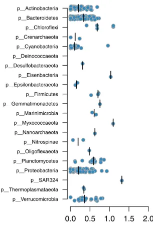
24–26,33

_{. As many as 320 out of the 352 BACLs obtained here}

could not be classified to the species-level, despite the fact that the

GTDB also includes species-level clades consisting solely of

genomes from uncultured organisms (MAGs and

single-amplified genomes). The corresponding numbers for

genus-and family-level were 180 genus-and 56. Thus, to our knowledge, the

dataset contains substantial novel genomic information. This is

also evident by plotting the phylogenetic distances between the

BACLs and their nearest neighbors in GTDB, where especially

phyla that are represented by a low number of BACL, such as

Eisenbacteria, Myxococcaeota and SAR324, display large

dis-tances to their nearest GTDB neighbors (Fig.

2

).

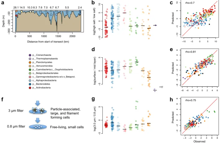
Ecological niche distributions. We used the different

metage-nomic sample sets to investigate how the BACLs were distributed

along various niche gradients in the Baltic Sea ecosystem (Fig.

3

).

Based on the surface samples from the Transect 2014 cruise,

spanning the salinity gradient from marine to near-freshwater

conditions, we derived a salinity niche-parameter for the BACLs

by calculating the ratio of their abundances in the high (>14 PSU)

vs. low (<6 PSU) salinity samples. Consistent with previous

stu-dies

24–26,33

_{, Actinobacteria and Betaproteobacteria where biased}

toward the lower range of the salinity gradient, while Alpha- and

Gammaproteobacteria where biased toward the upper range

(Fig.

3

b). By taking the ratio between the surface and mid layer

samples from the same cruise, we could compare the populations’

relative abundances in sunlit vs. dark conditions (Fig.

3

d). As

expected, phototrophic Cyanobacteria had a preference for the

upper sunlit water layer. In contrast, Planctomycetes, and even

more so Crenarcheaota and Thermoplasmataeota, showed a bias

towards deeper water layers. Other taxa such as Actinobacteria

and Bacteroidetes displayed more variability in their depth

pre-ferences, likely reflecting niche-partitioning within these phyla.

Finally, we used the data from different

filter-size fractions from

the Askö Time Series 2011 to assess the ratio between abundance

on >3.0

μm and 0.8–3.0 μm filter fractions (Fig.

3

g).

Actino-bacteria, Alpha- and Gammaproteobacteria were highly

under-represented within the 3.0

μm fraction, consistent with these cells

being primarily free-living and rarely particle-associated

34,35

_{. For}

Cyanobacteria, BACL annotated as Nostocales and

Pseudana-baenales, ie.

filamentous cyanobacteria, were enriched on the 3.0

μm filter, consistent with these forming filaments that were

captured on the

filter, while picocyanobacteria had distinctively

lower 3.0

μm/0.8 μm ratios. Bacteroidetes and Planctomycetes

displayed large variations, consistent with the fact that some

organisms from these groups are known to exist on particles

36,37

_.

Predicting niche from genome. We then proceeded to investigate

if the BACLs’ distributions along the above described niche

gra-dients could be directly predicted from their genomes. The large

number of BACLs allowed us to use a machine learning approach,

where we conducted training and predictions on separate sets of

BACLs. The encoded genes in each MAG were functionally

annotated using eggNOG orthologous groups

38

_{and a gene}

(egg-NOG) profile was calculated for each BACL based on the mean

profile of its MAGs (see Methods). We used various machine

learning approaches (ridge regression

39

_{, random forest}

40

_and

gradient boosting

41

_{) to predict the placement of each BACL along}

the niche gradients based on its gene profile. For all methods and

for all three niche gradients, the gene profile-predicted and actual

placements of BACLs were significantly correlated (Spearman

rank correlation,

ρ = 0.70–0.81, all P < 10

−16

; Fig.

3

c, e, h;

Sup-plementary Table 2).

While the above illustrates that bacterioplankton population

distributions can be predicted along specific a priori defined niche

gradients, it is reasonable to assume that each population is in fact

regulated by a multitude of abiotic and biotic factors. Defining

and measuring these factors, such as the availability of specific

dissolved organic matter compounds

42

or the presence of specific

viruses or predatory protists

43

_{, remains a major challenge in}

microbial oceanography. These factors will collectively determine

a population’s abundance in a sample, and thus its abundance

profile across multiple samples. Consequently, if two populations

display similar abundance profiles across samples they are likely

regulated in similar ways and hence likely to share the same

ecological niche. Analysing abundance profiles does not require

prior knowledge on regulating factors, as long as the samples

cover sufficient variation in these, and it allows a quantitative

assessment of niche sharing between populations. We retrieved

the abundance profile for each BACL over all the metagenome

samples (see Methods), and created a low dimensional virtual

niche space by running ordination on these profiles (Fig.

4

a–d).

The

first principal coordinates, or dimensions, in this space

explain most of the variation in abundance profile and should

thus correspond to the highest ecological variation. Among the

environmental parameters measured, temperature, oxygen and

silicate concentration were the most highly correlated to the

first

three dimensions, respectively (Fig.

4

c, d). However, dimensions

of lower rank did not correlate to any of the measured variables,

and are presumably driven by other factors. We used machine

learning to predict the placement of each BACL in this niche

p__Actinobacteria p__Bacteroidetes p__Chloroflexi p__Crenarchaeota p__Cyanobacteria p__Deinococcaeota p__Desulfobacteraeota p__Eisenbacteria p__Epsilonbacteraeota p__Firmicutes p__Gemmatimonadetes p__Marinimicrobia p__Myxococcaeota p__Nanoarchaeota p__Nitrospinae p__Oligoflexaeota p__Planctomycetes p__Proteobacteria p__SAR324 p__Thermoplasmataeota p__Verrucomicrobia

0.0

0.5

1.0

1.5

2.0

Fig. 2 Phylogenetic distances between BACLs and nearest GTDB neighbors. Each circle is a BACL represented by a MAG and the placement along the x-axis indicates phylogenetic distance to the nearest reference genome in the GTDB tree. Distributions are plotted separately for each phylum, with median values indicated by verticallines.

space based on its gene profile, again conducting training and

predictions on separate BACLs. As for the a priori defined niches,

predicted values were significantly correlated to the real values for

the

first ten principal coordinates of the niche space (Fig.

4

e–g

and Supplementary Table 2).

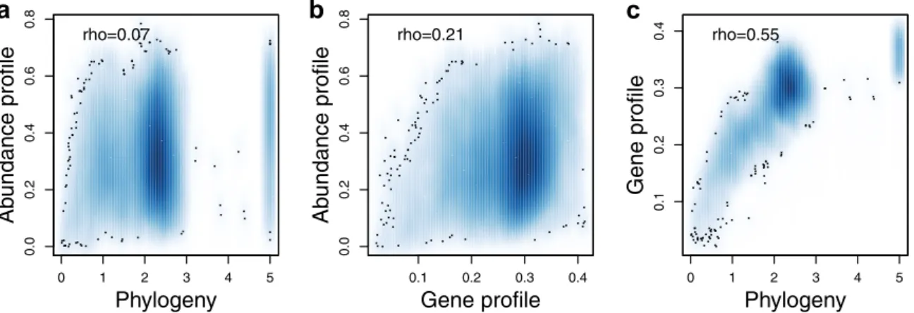
Gene content vs. phylogenetic signal. Since phylogeny is known

to be related to both gene content

44

_{and abundance distribution}

5

_,

it is possible that the machine learning models are merely picking

up a phylogenetic signal. Therefore, we also predicted the

pla-cement of BACLs in the niche space using phylogenetic

infor-mation, applying a method based on ancestral state estimation

45

_.

This method also gave significant correlations to the real values,

however with lower correlations for 8 of the

first 10 principal

coordinates compared to gene-content-based predictions with the

machine learning approach that worked best (gradient boosting;

Supplementary Table 2). Thus, the gene-based models appear to

pick up genetic signals that are directly related to ecology and not

only to phylogeny. To further investigate how ecology is reflecting

phylogeny as compared to gene content, we correlated pairwise

dissimilarity in abundance profile to either pairwise phylogenetic

distance or gene profile dissimilarity. A weak but highly

sig-nificant correlation was found between abundance profile

dissimilarity and phylogenetic distance (Fig.

5

a), similar to what

was previously observed in a time-series analysis of

bacter-ioplankton

5

_{. However, this correlation was slightly weaker than}

between abundance profile dissimilarity and gene profile

dis-similarity (Fig.

5

b), despite that pairwise dissimilarity in gene

profile was highly correlated with phylogenetic distance (Fig.

5

c).

The stronger correlation between abundance profile and gene

content was confirmed by partial correlations, where abundance

profile dissimilarity remained correlated with gene content

dis-similarity when controlling for phylogenetic distance (partial

Mantel test, Spearman

ρ = 0.21, P = 10

−4

, number of

permuta-tions

= 10

4

_{), while the correlation between abundance profile}

dissimilarity and phylogenetic distance disappeared when

con-trolling for gene content dissimilarity (ρ = −0.06, P = 1).

The above gene profile-based niche predictions were conducted

using the whole community of BACLs for defining the niche

space. We

finally performed the same type of analysis, but now

generating the virtual niche space and running the machine

learning on one taxonomic division at a time, to see if we could

resolve more subtle differences in niche based on more subtle

differences in gene content. For the clades with most BACLs

(Actinobacteria, Bacteroidetes, Alpha- and

Gammaproteobac-teria) the

first three principal coordinates could be predicted fairly

well, with mean correlation coefficients between predicted and

0 500 1000 1500 2000

350

200

50

Distance from start of transect (km)

Depth (m)

Particle-associated, large, and filament forming cells Free-living, small cells 3 µm filter

0.8 µm filter

log(3.0 µm / 0.8 µm)

log(surface / mid layer)

log(high salt / low salt)

p__Actinobacteria p__Bacteroidetes c__Alphaproteobacteria

c__Gammaproteobacteria w/o o_Betaprot. o__Betaproteobacteriales p__Cyanobacteria;c__Oxyphotobacteria p__Verrucomicrobia p__Planctomycetes p__Thermoplasmataeota p__Crenarchaeota Predicted Predicted Predicted Observed

a

b

c

d

e

f

g

h

28.1 14.5 10.3 8.3 7.6 7.0 6.7 6.7 5.5 2.4 10 50 5 1 0 5 0 5 50 5 10 5 0 5 10 10 50 5 1 0 _rho=0.7 8 6 4 2 0 2 4 6 8 6 4 20 2 46 rho=0.81 4 2 0 2 4 6 8 4 20 2 4 6 8 rho=0.75

Fig. 3 Observed and predicted distributions of BACLs along selected niche gradients. a Side view of Transect 2014 with surface and mid layer samples

indicated by circles, colored according to salinity as in Fig.1. Numbers above the graph indicate salinity in the surface layer samples.b Ratio between

abundance in the high and low salinity surface samples of the Transect 2014 cruise. Values are log ratios of the mean abundances in the 14.5 and 28 PSU

and the 2.4 and 5.5 PSU samples. Distributions are plotted separately for each taxon, with median values indicated by horizontal lines.c Machine learning

predicted vs. observed log ratio between abundance in the high and low salinity samples.d Ratio between abundance in surface and abundance in mid layer

water samples from the Transect 2014 cruise. Values are average log ratios for the 10 surface/mid sample pairs. e Machine learning predicted vs. observed

log ratio between abundance in surface and mid layer samples.f Cartoon indicating difference between cells captured on 3 and 0.8_{μm filters by sequential}

filtration. g Ratio between abundance on 3.0 μm and abundance on 0.8 μm filters in the Askö Time Series 2011 sample set. Values are average log ratios for

the six 3.0μm/0.8 μm sample pairs. h Machine learning predicted vs. observed log ratio between abundance on 3.0 and 0.8 μm filters. Machine learning

predictions performed by gradient boosting using gene (eggNOG) pro_{files. Low abundance BACLs were excluded from the graphs in b, d, g (see Methods).}

real values of 0.61 using gradient boosting (Supplementary

Table 3). Again, gene-content-based predictions were generally

better than predictions based on phylogenetic information

(Supplementary Table 3).

Discussion

The results presented here demonstrate a strong link between an

organism’s encoded genes and its ecological niche. Already in the

early days of microbial genomics, a relationship between gene

content and phylogeny was demonstrated

44

_{and phylogenetic}

relatedness has been correlated with ecological relatedness in

both macro- and microorganisms

3–5,46–50

. Moreover, genomic

approaches have correlated variation in gene content in natural

microbial populations to varying environmental conditions

51–53

,

and clustering prokaryotes based on what genes they encode has

been shown to form groups with shared functional and

envir-onmental attributes

54

. However, to our knowledge, our study is

the

first systematic prediction of ecological niche as manifested in

species distributions based solely on genomic information. The

placements along the

first dimensions in the virtual niche space

and along the a priori defined gradients could be estimated with

correlation coefficients of ~0.7, meaning that around 50% of the

variation along these dimensions could be explained by gene

content alone. Since the placement along the

first principal

a b

c

d

e

f

g

Sample BA CL 1 2 3 4 5 6 7 8 9 10 V a riance e xplained 0.00 0.02 0.04 0.06 0.08 0.10 PC 0.4 0.2 0.0 0.2 0.2 0.1 0.0 0.1 0.2 PC1 PC2 1 2 3 4 5 6 7 8 10₉ 0.4 0.2 0.0 0.2 0.2 0.1 0.0 0.1 0.2 PC1 PC3 1 2 3 4 5 6 7 8 9 10 0.4 0.2 0.0 0.2 0.4 0.2 0 .0 0.2 Observed PC1 Predicted PC1 rho=0.74 0.3 0.1 0.0 0.1 0.2 0.3 0.2 0.1 0 .0 0.1 0 .2 Observed PC2 Predicted PC2 rho=0.7 0.3 0.1 0.0 0.1 0.2 0.3 0.3 0.1 0 .0 0.1 0 .2 0.3 Observed PC3 Predicted PC3 rho=0.64

Fig. 4 Observed and predicted distributions of BACLs along principal axes of abundance variation. a BACL abundance profiles (one BACL per line; the

99 most abundant BACL shown) across all 124 samples, with dot size proportional to log abundance in the sample, using the same color schema as in Fig.3

but with additional taxa shown in black.b–d Principal coordinates analysis of BACL abundance profiles, with b displaying proportion of variation explained

by the tenfirst principal coordinates (PC) and c, d plotting the BACLs along the first three principal coordinates. The arrows indicate relationships between

the principal coordinates and measured environmental parameters (see Methods), where the numbers correspond to 1: salinity; 2: depth; 3: oxygen; 4:

temperature; 5:filter size; 6: nitrate; 7: phosphate; 8: silicate; 9: chlorophyll a; 10: dissolved organic carbon. e–g Machine learning predicted (gradient

boosting using gene profiles) vs. observed values of principal coordinate scores, with e displaying results for PC1, f for PC2 and g for PC3. Rho-values

indicate Spearman rank correlation coefficients between predicted and observed values (all correlations P < 10-16_{). Prediction results for PC1–PC10 using}

different machine learning algorithms can be found in Supplementary Table 2.

0 1 2 3 4 5 0.0 0.2 0.4 0.6 0.8

Phylogeny

Ab

undance profile

rho=0.07 0.1 0.2 0.3 0.4 0.0 0.2 0.4 0.6 0.8

Gene profile

Ab

undance profile

rho=0.21 0 1 2 3 4 5 0.1 0.2 0.3 0.4

Phylogeny

Gene profile

rho=0.55

a b c

Fig. 5 Relationships between ecology, phylogeny and gene-content. a Abundance profile dissimilarity (y-axis) vs. phylogenetic distance (x-axis).

b Abundance pro_{file dissimilarity (y-axis) vs. gene profile dissimilarity (x-axis). c Gene profile dissimilarity (y-axis) vs. phylogenetic distance (x-axis).}

Rho-values indicate Spearman rank correlation coefficients. All correlations were significant (Mantel test, P = 10−4, number of permutations= 104_{). The}

coordinates of the niche space were generally better predicted

using gene content than phylogenetic information, our results

indicate that gene content is superior to phylogenetic information

for predicting ecological niche, highlighting the importance of

genomic data for advancing the

field of microbial ecology. This

was also supported by the direct correlations between abundance

profile distances and phylogenetic and gene content distances,

respectively. The stronger association between ecology and gene

content may appear logical, given that gene content does not

strictly follow phylogenetic trajectories due to lateral gene transfer

events

55,56

. On the other hand, although the MAGs used for the

analysis were estimated to be of rather high quality, the gene

content-based models should suffer from some extent of

incompleteness and impurities in the genomic information due to

shortcomings of the assembly and binning processes. In our

analysis we predicted the abundance distributions of species-level

genome clusters. As methods for strain-level genome

recon-structions develop

57,58

the approach can likely be improved by

using more precise information on gene content and abundance

distributions of individual strains, since even a single gene can

have dramatic effect on niche. Also, genes were grouped in rather

broad orthologous groups, that are sometimes functionally

het-erogeneous. Follow-up studies could address if higher accuracy

predictions may be achieved by using more refined gene function

definitions, or even genotypic variation. Despite the room for

further methodological improvements, our analyses demonstrate

a strong link between an organism’s gene content and its ecology.

The approach developed here may in the future be applicable in

environmental management, for example for predicting the

abundance distributions of alien species arriving in a new

eco-system. It is also possible that species distribution models (SDM),

that today are typically built on environmental data alone

59

_{, can}

be improved by incorporating genomic information. Whilst we

applied the approach to prokaryotes, it should be applicable also

for microbial eukaryotes as more genomic information is

gath-ered for these.

Methods

Sample retrieval and DNA sequencing. Samples included within this study are

divided intofive sample sets named Askö Time Series 2011, Redoxcline 2014,

Transect 2014, LMO Time Series 2013–2014 and Coastal Transect 2015(Fig.1a).

Metagenome data for three of these have previously been published: Askö Time

Series 201160_{, Redoxcline 2014}33_{, Transect 2014}33_{; and two are new to this}

pub-lication: LMO Time Series 2013–2014 and Coastal Transect 2015. For the published

sample sets, only a brief description of sample retrieval is given here. For detailed descriptions, the reader is directed to the respective publication.

The Askö Time Series 201160_{samples (n= 24) were collected on six occasions}

between 14 June and 30 August in 2011. On each occasion, the samples were

sequentiallyfiltered through 200, 3.0, 0.8 and 0.1 µm filters. DNA was sequenced

from the 3.0, 0.8 and 0.1 µmfilters, as well from the water passing the 0.1 µm filter.

The Redoxcline 201433_{samples (n= 14) target the transition between oxic and}

anoxic water and were collected on three occasions in 2014, from the Gotland Deep

on October 18 (n= 2) and October 26 (n = 8) and from the Boknis Eck61_station

on September 23 (n= 4). The October 18 samples were captured on a 0.2 µm filter

without pre-filtration while all other samples were filtered either on 3.0 µm filter without filtration (n = 6), or on a 0.2 µm filter using 3.0 µm filter for pre-filtration (n = 6).

The Transect 201433_{samples (n= 30) were collected during a cruise in June}

2014. Samples were taken from three different depths, spanning the oxygenated zone, at ten stations covering the horizontal salinity gradient. Samples were

captured on a 0.2 µmfilter without pre-filtration.

The LMO Time Series 2013–2014 samples (n = 22) were collected from the Linnaeus Microbial Observatory station 10 km east of Öland (Latitude 56.938436,

Longitude 17.06204) from January 2013 to December 201462_{. 10 liter samples from}

surface water (2 m depth) were collected using a Ruttner sampler and transported to the laboratory in carefully acid rinsed polycarbonate containers. 3–5 liter of

seawater werefiltered through 0.22 µm filters (Sterivex, Millipore) to harvest cells,

following pre-filtration through 3.0 µm filters (Poretics polycarbonate, GVS Life

Sciences). DNA was extracted using the protocol by Boström et al.63_{, as modified}

by Bunse et al.64_.

The Coastal Transect 2015 samples (n= 34) were collected during a cruise with

the R/V Poseidon (Cruise POS488) organised by the Leibniz Institute for Baltic Sea

Research, Warnemünde, in August/September 2015 from stations located closer to the coastline compared to the Transect 2014 stations. 1 liter samples were collected

from surface water (1.7–4.0 m depth) and cells were captured on 0.2 µm filters

without pre-filtration. DNA was extracted as earlier described for the Transect 2014

samples33_.

All sequencing libraries were prepared with the Rubicon ThruPlex kit (Rubicon Genomics, Ann Arbor, Michigan, USA) according to the instructions of the manufacturer and sequenced at the National Genomics Infrastructure (NGI) at Science for Life Laboratory, Stockholm, Sweden, using HiSeq 2500 high-output producing an average of 44 million pair-end read pairs per sample.

Sequence preprocessing, assembly and quanti_{fication. All samples were}

pre-processed by the same procedure, removal of low quality bases using cutadapt65

with parameters“-q 15,15” followed by adapter removal with parameters “-n 3

–minimum-length 31 -a AGATCGGAAGAGCACACGTCTGAACTCCAGTC AC -G ^CGTGTGCTCTTCCGATCT -A AGATCGGAAGAGCGTCGTGTAGGG AAAGAGTGT”. These settings ensured that reads shorter than 31 bases after

adapter trimming were discarded. Furthermore, the readfiles were screened for

artificial PCR duplicates using FastUniq66_{with default parameters.}

After preprocessing, the samples were individually assembled using

MEGAHIT67_{version 1.1.2 with the–meta-sensitive option. For each sample,}

contigs longer than 20 kb were then cut up from the start into non-overlapping parts of 10 kilobases, such that the last piece was between 10 and 20 kilobases long.

This was performed using the script“cut_up_fasta.py” from the CONCOCT29

repositoryhttps://github.com/binpro/CONCOCT.

The process continued sample-wise with quantification of each processed

assemblyfile using all read files. The cut-up contigs, as well as all short contigs,

were used as input to the index method of Kallisto28_{version 0.43.0. The}

quantifications were performed using the “quant” method of Kallisto on each of the

124 samples in a cross-wise manner, resulting in 124 × 124= 15376 runs. To

transform the estimated counts, which is reported by Kallisto, into approximate

coverage values, these count values were multiplied by 200 (a simplification,

representing the read pair length) and divided by the contig length. This step was

performed using the script“kallisto_concoct/input_table.py” from the toolbox

repositoryhttps://github.com/EnvGen/toolbox(https://doi.org/10.5281/

zenodo.1489089).

One of the Transect 2014 samples (P1994_109) was accidently not assembled and MAGs were not binned from it, but the sample was included in the

quantification of contigs of other samples. Hence binning was done on 123 samples

but using quantification information from 124 samples.

Binning and quality screening. The SpeedUp_Mp branch of CONCOCT was used for binning of the individual samples. Bin assignments by CONCOCT for cut-up contigs were re-evaluated so that all parts of long contigs were placed in the

same bin by majority vote. This was done using the script

“scripts/concoct/mer-ge_cutup_clustering.py” within the toolbox repositoryhttps://github.com/envgen/

toolbox(https://doi.org/10.5281/zenodo.1489089). Based on this second bin

assignment, all individual bins were extracted as fasta-files, using the original

pre-cut-up contigs. To identify prokaryotic Metagenome Assembled Genomes

(MAGs), these bins were evaluated using CheckM30_{version 1.0.7. Bins with an}

estimated completeness of≥75% and estimated contamination ≤5% were approved

and considered prokaryotic MAGs, fulfilling the criteria of being “substantially complete” (≥70%) and having ‘low contamination’ (≤5%), according to the

con-trolled vocabulary of draft genome quality30_.

Fragment recruitment. Proportion of metagenome reads recruited to MAGs was calculated by randomly sampling 1000 forward (R1) reads from each sample and

matching against the contigs of all MAGs, including also the LMO 2012 MAGs22_,

with BLASTN, using≥97% identity and alignment length ≥90% of read length as

thresholds for counting a read as matching.

Clustering and taxonomic annotation of MAGs. Sequence similarity between all MAGs (including those retrieved here and those retrieved in a previous study from

station LMO22_{) was estimated using fastANI}68_{using the default k-mer length of 16.}

These sequence similarity estimates were used to cluster the MAGs at 96.5% identity level using average-linkage hierarchical clustering using SciPy version 0.17.0. Taxonomic assignment for all prokaryotic MAGs was performed using the

classify_wf method of Genome Taxonomy Database Toolkit32_{(GTDB-Tk) using}

release version 80 of the database and version 0.0.4b1 of the toolkit. Each cluster of prokaryotic MAGs was assigned an identifier BACLX, following the nomenclature

established in Hugerth et al.22_.

When analysing how BACLs were distributed over niches in the ecosystem and predicting niches, a single MAG was chosen as representative for each MAG cluster. This choice was based on the estimated completeness and contamination levels, where the MAG with highest completeness after subtracting its contamination was chosen. The selected MAGs had a mean estimated completeness and contamination of 92.2% and 2.2%, respectively.

Evaluation of binning based on internal standard. Comparisons between the obtained internal standard genome bins and the reference genome (Thermus thermophilus str. HB8; accession number GCF_000091545.1) were performed using the dnadiff script from MUMmer version 3.23, comparing to the main reference genome and the two plasmids separately.

Genome annotations. Genes were predicted in the MAGs with Prodigal (v.2.6.3), running the program on each MAG separately in default single genome mode. Functional annotation of genes were conducted using eggNOG mapper version

1.0.369_{. Gene profiles were obtained by counting the number of occurence of each}

eggNOG with a“@NOG” suffix in each genome. In total 35,593 such unique

eggNOGs were found, of which 4115 were COGs. The gene profile of a BACL was calculated by taking the average of the gene profiles of the MAGs in the BACL.

Pairwise dissimilarities of gene profiles between BACLs were calculated using

Spearman rank correlations, where the gene profile dissimilarity = (1 − ρ)/2, and

whereρ is the Spearman correlation coefficient.

Abundance pro_{files. The abundance of a MAG in a sample was calculated by}

taking the average of the Kallisto estimated contig abundances, weighted by the contig lengths, and converted into a coverage per million read-pairs value by dividing by the number of million read-pairs that were mapped from the sample.

The abundance profile of the representative MAG for a BACL was used as

abundance profile for the BACL (abundance profiles were highly correlated between MAGs within BACLs, average Spearman correlation coefficient = 0.98).

Pairwise dissimilarities of abundance profiles between BACLs were calculated using

Spearman rank correlations, analogously to how gene profile dissimilarities were calculated. Ordination of abundance profiles was conducted using Principal

Coordinates Analysis (PCoA) on the abundance profile dissimilarity matrix using

‘Cailliez’ correction with the R70_{package ape}71_{. To relate the PCoA coordinates to}

environmental factors (the arrows of Fig. 4c, d), the Spearman correlation

coeffi-cients between each BACL abundance profile and each of the measured

environ-mental parameters werefirst calculated. Next, the Spearman correlation between

these correlation coefficients and the BACLs positioning along the PCoA coordi-nates were calculated. The end-point of the arrow is proportional to the latter correlation: An arrow pointing far to the right indicates that BACLs to the right in the plot are positively correlated with the environmental factor, while those to the left are negatively correlated. An arrow pointing far to the left indicates that BACL to the left in the plot are positively correlated, while those to the right are negatively correlated.

Phylogenetic distances. Phylogenetic distances between MAGs were calculated using the R package ape based on the GTDB phylogenetic trees (one for Bacteria

and one for Archaea) with MAGs inserted using GTDB-Tk32_{using release version}

80 of the database and version 0.0.4b1 of the toolkit. Phylogenetic distances between each bacterial-archaeal pair was set to an arbitrary level of 5 (higher than

any of the distances observed within each domain-specific tree). Phylogenetic trees

were visualised with GraPhlAn72_.

Ecological predictions. In order to lower the risk of miscalculating abundances

due to non-specific contig quantifications, BACLs including any MAG with >0.95

ANI to any MAG of another BACL were excluded, leaving 342 BACL for the analysis. All of these were included for the predictions of PCoA coordinate scores (or the subset of these that had the correct taxonomic annotation, when performing

taxon-specific predictions). For predicting the a priori defined niches, BACLs

among these that displayed low abundances were further removed: When pre-dicting abundance ratio between high and low salinity samples from the Transect 2014 cruise, only BACLs displaying a highest relative abundance of >0.01 coverage

per million read-pairs among these samples were included (n= 243). When

pre-dicting the average log ratio between the abundance in surface and abundance in mid layer water in the Transect 2014 cruise, only BACLs displaying a highest coverage of >0.05 coverage per million read-pairs among these 20 samples where

included (n= 246). When predicting the average log ratio between the abundance

on 3.0μm and abundance on 0.8 μm filters for the Askö Time Series 2011 sample

set, only BACL displaying a highest coverage of >0.01 coverage per million

read-pairs among these 12 samples where included (n= 227). The same inclusion

cri-teria were used when plotting BACLs along these niche gradients in Fig.3.

Ecological predictions were conducted using either gene profiles or phylogenetic

information. For gene profile-based predictions, gene profiles (calculated as

described above) werefiltered to only include those eggNOGs that were present in

at least 10% of all BACL, resulting in profiles of 3476 eggNOGs of which 2360 were

COGs. Gene profile-based predictions were conducted using ridge regression,

random forests and gradient boosting. Ridge regressions were performed using the

R package glmnet39_{with the alpha parameter set to 0. The hyperparameter lambda}

was tuned using cross validation within each training set, and the lambda value giving the minimum mean error was used. Random Forest regressions were

conducted using the R package randomForest73_{, using number of trees set to 2000}

(other parameters kept at default values). Gradient boosting regressions were

conducted using the R package gbm74_{using a gaussian loss function. The}

parameter settings for number of trees (‘n.trees’), learning rate (‘shrinkage’),

maximum depth of each tree (‘interaction.depth’) and minimum number of observations in the terminal nodes (‘n.minobsinnode’) were optimised manually

based on the success of predicting the scores of thefirst PCoA coordinate (with all

BACL) using different settings. These setting (n.trees= 10000, shrinkage = 0.001,

interaction.depth= 2, n.minobsinnode = 1) were subsequently used for all

predictions.

Predictions based on phylogenetic information were conducted using the R

package picante45_{using ancestral state estimation to infer unknown trait values for}

taxa based on the values observed in their evolutionary relatives75,76_{. The GTDB}

trees with inserted MAGs were used for this purpose, byfirst removing all branches

corresponding to other genomes than the BACL representative MAGs. For ridge regression and gradient boosting we used 10-fold cross-validation between the predicted and observed values. In other words, the set of BACLs were randomly partitioned into ten equally sized subsets. Of the 10 subsets, a single subset was kept as the validation data, and the remaining nine subsets were used as training data. The cross-validation process was then repeated ten times, with each of the ten subsets used once as the validation data. This way, the prediction for each BACL was validated once. For random forests we compared the out-of-bag predictions with the observed values, where the out-of-bag predictions are the predictions based on trees trained on BACLs other than the BACLs under validation. For validations, predicted values were compared with actual values using Spearman rank correlation for all types of predictions.

Statistics and reproducibility. Spearman rank correlation was used to evaluate ecological niche predictions and (partial) Mantel test to assess correlations between abundance profile dissimilarity, gene profile dissimilarity and phylogenetic distance.

Reporting summary. Further information on research design is available in the Nature Research Reporting Summary linked to this article.

Data availability

The contigs from the individual samples and the MAG sequences were submitted to ENA hosted by EMBL-EBI under the study accession number PRJEB34883. Note that contigs stemming from the internal standards genome (Thermus thermophilus) are included in the contigs for the Transect 2014 samples. The preprocessed sequencing reads from the LMO Time Series 2013–2014 and Coastal Transect 2015 samples were submitted to ENA under the same study accession number (PRJEB34883). The preprocessed sequencing reads from the Transect 2014and Redoxcline 2014 samples were published elsewhere33_{and are available at ENA under the study accession number PRJEB22997.}

The raw sequencing reads from the Askö Time Series 2011 were published elsewhere60

and are available at NCBI under the study accession number SRP077551.

Received: 3 July 2019; Accepted: 25 February 2020;

References

1. Hutchinson, G. E. Concluding remarks. Cold Spring Harb. Symposia Quant.

Biol. 22, 415–427 (1957).

2. Webb, C. O. Exploring the phylogenetic structure of ecological communities:

an example for rain forest trees. Am. Nat. 156, 145–155 (2000).

3. Horner-Devine, M. C. & Bohannan, B. J. M. Phylogenetic clustering and

overdispersion in bacterial communities. Ecology 87, S100–8 (2006).

4. Burns, J. H. & Strauss, S. Y. More closely related species are more ecologically

similar in an experimental test. Proc. Natl Acad. Sci. USA 108, 5302–5307 (2011).

5. Andersson, A. F., Riemann, L. & Bertilsson, S. Pyrosequencing reveals

contrasting seasonal dynamics of taxa within Baltic Sea bacterioplankton

communities. ISME J. 4, 171–181 (2010).

6. Martiny, J. B. H., Jones, S. E., Lennon, J. T. & Martiny, A. C. Microbiomes in

light of traits: A phylogenetic perspective. Science 350, aac9323–aac9323 (2015).

7. Cavender-Bares, J., Kozak, K. H., Fine, P. V. A. & Kembel, S. W. The merging

of community ecology and phylogenetic biology. Ecol. Lett. 12, 693–715 (2009).

8. Hyatt, D. et al. Prodigal: prokaryotic gene recognition and translation

initiation site identification. BMC Bioinforma. 11, 119 (2010).

9. Ye, Y. & Doak, T. G. A parsimony approach to biological pathway

reconstruction/inference for genomes and metagenomes. PLoS Comput. Biol. 5, e1000465 (2009).

10. Weimann, A. et al. From genomes to phenotypes: traitar, the microbial trait

analyzer. mSystems. 1, e00101–16 (2016).

11. Brbić, M. et al. The landscape of microbial phenotypic traits and associated

12. Jensen, D. B. & Ussery, D. W. Bayesian prediction of microbial oxygen requirement. F1000Res. 2, 184 (2013).

13. Jensen, D. B., Vesth, T. C., Hallin, P. F., Pedersen, A. G. & Ussery, D. W. Bayesian prediction of bacterial growth temperature range based on genome sequences. BMC Genomics 13, S3 (2012).

14. Lauro, F. M. et al. The genomic basis of trophic strategy in marine bacteria.

Proc. Natl Acad. Sci. USA 106, 15527–15533 (2009).

15. Falkowski, P. G., Fenchel, T. & Delong, E. F. The microbial engines that drive Earth’s biogeochemical cycles. Science 320, 1034–1039 (2008).

16. Venter, J. C. et al. Environmental genome shotgun sequencing of the Sargasso Sea. Science 304, 66–74 (2004).

17. Sunagawa, S. et al. Structure and function of the global ocean microbiome. Science 348, 1261359 (2015).

18. Quince, C., Walker, A. W., Simpson, J. T., Loman, N. J. & Segata, N. Shotgun metagenomics, from sampling to analysis. Nat. Biotechnol. 35, 833–844 (2017).

19. Delmont, T. O. et al. Nitrogen-fixing populations of Planctomycetes and

Proteobacteria are abundant in surface ocean metagenomes. Nat. Microbiol. 3,

804–813 (2018).

20. Tully, B. J., Graham, E. D. & Heidelberg, J. F. The reconstruction of 2,631 draft metagenome-assembled genomes from the global oceans. Sci. Data 5, 170203 (2018).

21. Linz, A. M. et al. Freshwater carbon and nutrient cycles revealed through reconstructed population genomes. PeerJ 6, e6075 (2018).

22. Hugerth, L. W. et al. Metagenome-assembled genomes uncover a global brackish microbiome. Genome Biol. 16, 279 (2015).

23. Snoeijs-Leijonmalm, P., Schubert, H. & Radziejewska, T. Biological Oceanography of the Baltic Sea. (Springer Science & Business Media, 2017).

24. Herlemann, D. P. et al. Transitions in bacterial communities along the 2000

km salinity gradient of the Baltic Sea. ISME J. 5, 1571–1579 (2011).

25. Dupont, C. L. et al. Functional tradeoffs underpin salinity-driven divergence in microbial community composition. PLoS ONE 9, e89549 (2014). 26. Hu, Y. O. O., Karlson, B., Charvet, S. & Andersson, A. F. Diversity of Pico- to

Mesoplankton along the 2000 km Salinity Gradient of the Baltic Sea. Front. Microbiol. 7, 679 (2016).

27. Lindh, M. V. et al. Disentangling seasonal bacterioplankton population dynamics by high-frequency sampling. Environ. Microbiol. 17, 2459–2476 (2015).

28. Bray, N. L., Pimentel, H., Melsted, P. & Pachter, L. Near-optimal probabilistic RNA-seq quantification. Nat. Biotechnol. 34, 525–527 (2016).

29. Alneberg, J. et al. Binning metagenomic contigs by coverage and composition.

Nat. Methodshttps://doi.org/10.1038/nmeth.3103(2014).

30. Parks, D. H. et al. CheckM: assessing the quality of microbial genomes recovered from isolates, single cells, and metagenomes 5. Genome Res. 25,

1043–1055

31. Varghese, N. J. et al. Microbial species delineation using whole genome

sequences. Nucleic Acids Res. 43, 6761–6771 (2015).

32. Parks, D. H. et al. A standardized bacterial taxonomy based on genome phylogeny substantially revises the tree of life. Nat. Biotechnol. 36, 996–1004 (2018).

33. Alneberg, J. et al. BARM and BalticMicrobeDB, a reference metagenome and interface to meta-omic data for the Baltic Sea. Sci. Data 5, 180146 (2018). 34. Newton, R. J., Jones, S. E., Eiler, A., McMahon, K. D. & Bertilsson, S. A guide

to the natural history of freshwater lake bacteria. Microbiol. Mol. Biol. Rev. 75,

14–49 (2011).

35. Giovannoni, S. J., Cameron Thrash, J. & Temperton, B. Implications of

streamlining theory for microbial ecology. ISME J. 8, 1553–1565 (2014).

36. Fernández-Gómez, B. et al. Ecology of marine Bacteroidetes: a comparative

genomics approach. ISME J. 7, 1026–1037 (2013).

37. DeLong, E. F., Franks, D. G. & Alldredge, A. L. Phylogenetic diversity of aggregate-attached vs. free-living marine bacterial assemblages. Limnol. Oceanogr. 38, 924–934 (1993).

38. Huerta-Cepas, J. et al. eggNOG 4.5: a hierarchical orthology framework with improved functional annotations for eukaryotic, prokaryotic and viral sequences. Nucleic Acids Res. 44, D286–93 (2016).

39. Friedman, J., Hastie, T. & Tibshirani, R. Regularization paths for generalized linear models via coordinate descent. J. Stat. Softw. 33, 1–22 (2010). 40. Breiman, L. Random forests. Mach. Learn. 45, 5–32 (2001).

41. Hastie, T., Tibshirani, R. & Friedman, J. The Elements of Statistical Learning, ser. (Springer, 2001).

42. Moran, M. A. et al. Deciphering ocean carbon in a changing world. Proc. Natl

Acad. Sci. USA 113, 3143–3151 (2016).

43. Chow, C.-E. T., Kim, D. Y., Sachdeva, R., Caron, D. A. & Fuhrman, J. A. Top-down controls on bacterial community structure: microbial network analysis of bacteria, T4-like viruses and protists. ISME J. 8, 816–829 (2014). 44. Huynen, M. A. & Bork, P. Measuring genome evolution. Proc. Natl Acad. Sci.

USA 95, 5849–5856 (1998).

45. Kembel, S. W. et al. Picante: R tools for integrating phylogenies and ecology. Bioinformatics 26, 1463–1464 (2010).

46. Gilbert, G. S. & Webb, C. O. Phylogenetic signal in plant pathogen-host range.

Proc. Natl Acad. Sci. USA 104, 4979–4983 (2007).

47. Goberna, M. & Verdú, M. Predicting microbial traits with phylogenies. ISME

J. 10, 959–967 (2016).

48. Martiny, A. C., Treseder, K. & Pusch, G. Phylogenetic conservatism of functional traits in microorganisms. ISME J. 7, 830–838 (2013).

49. Herlemann, D. P. R., Lundin, D., Andersson, A. F., Labrenz, M. & Jürgens, K. Phylogenetic signals of salinity and season in bacterial community composition across the salinity gradient of the Baltic Sea. Front. Microbiol. 7, 1883 (2016).

50. Fierer, N., Bradford, M. A. & Jackson, R. B. Toward an ecological classification of soil bacteria. Ecology 88, 1354–1364 (2007).

51. Coleman, M. L. & Chisholm, S. W. Ecosystem-specific selection pressures revealed through comparative population genomics. Proc. Natl Acad. Sci. USA

107, 18634–18639 (2010).

52. Denef, V. J. et al. Proteogenomic basis for ecological divergence of closely related bacteria in natural acidophilic microbial communities. Proc. Natl Acad.

Sci. USA 107, 2383–2390 (2010).

53. Hunt, D. E. et al. Resource partitioning and sympatric differentiation among closely related bacterioplankton. Science 320, 1081–1085 (2008).

54. Suen, G., Goldman, B. S. & Welch, R. D. Predicting prokaryotic ecological niches using genome sequence analysis. PLoS ONE 2, e743 (2007). 55. Ochman, H., Lawrence, J. G. & Groisman, E. A. Lateral gene transfer and the

nature of bacterial innovation. Nature 405, 299–304 (2000). 56. Smillie, C. S. et al. Ecology drives a global network of gene exchange

connecting the human microbiome. Nature 480, 241–244 (2011).

57. Quince, C. et al. DESMAN: a new tool for de novo extraction of strains from metagenomes. Genome Biol. 18, 181 (2017).

58. Scholz, M. et al. Strain-level microbial epidemiology and population genomics from shotgun metagenomics. Nat. Methods 13, 435 (2016).

59. Elith, J. & Leathwick, J. R. Species distribution models: ecological explanation and prediction across space and time. Annu. Rev. Ecol., Evolution, Syst. 40, 677–697 (2009).

60. Larsson, J. et al. Picocyanobacteria containing a novel pigment gene cluster dominate the brackish water Baltic Sea. ISME J. 8, 1892–1903 (2014). 61. Bange, H. W. & Malien, F. Hydrochemistry from time series station

Boknis Eck from 1957 to 2014.https://doi.org/10.1594/PANGAEA.855693

(2015).

62. Bunse, C. et al. High frequency multi-year variability in baltic sea microbial plankton stocks and activities. Front. Microbiol. 9, 3296 (2019).

63. Boström, K. H., Simu, K., Hagström, Å., Riemann, L. Optimization of DNA extraction for quantitative marine bacterioplankton community analysis.

Limnology and Oceanography: Methods 2, 365–373 (2004)

64. Bunse, C. et al. Spatio-Temporal Interdependence of Bacteria and Phytoplankton during a Baltic Sea Spring Bloom. Frontiers in Microbiology 7 (2016).

65. Martin, M. Cutadapt removes adapter sequences from high-throughput sequencing reads. EMBnet. J. 17, 10–12 (2011).

66. Xu, H. et al. FastUniq: a fast de novo duplicates removal tool for paired short reads. PLoS ONE 7, e52249 (2012).

67. Li, D., Liu, C.-M., Luo, R., Sadakane, K. & Lam, T.-W. MEGAHIT: an ultra-fast single-node solution for large and complex metagenomics assembly via

succinct de Bruijn graph. Bioinformatics 31, 1674–1676 (2015).

68. Jain, C., Rodriguez-R, L. M. & Phillippy, A. M. High-throughput ANI Analysis of 90K Prokaryotic Genomes Reveals Clear Species Boundaries. bioRxiv (2017).

69. Huerta-Cepas, J. et al. Fast genome-wide functional annotation through

orthology assignment by eggNOG-Mapper. Mol. Biol. Evol. 34, 2115–2122

(2017).

70. Team, R. C. & Others. R: A language and environment for statistical computing. (2013).

71. Paradis, E., Claude, J. & Strimmer, K. APE: analyses of phylogenetics and evolution in R language. Bioinformatics 20, 289–290 (2004).

72. Asnicar, F., Weingart, G., Tickle, T. L., Huttenhower, C. & Segata, N. Compact graphical representation of phylogenetic data and metadata with GraPhlAn. PeerJ 3, e1029 (2015).

73. Breiman, L., Cutler, A., Liaw, A. & Wiener, M. Package randomForest.

Software available at:http://stat-www.berkeley.edu/users/breiman/

RandomForests(2011).

74. Ridgeway, G. & Others. gbm: Generalized boosted regression models. R. package version 1, 55 (2006).

75. Kembel, S. W., Wu, M., Eisen, J. A. & Green, J. L. Incorporating 16S gene copy number information improves estimates of microbial diversity and abundance. PLoS Comput. Biol. 8, e1002743 (2012).

76. Garland, T. & Ives, A. R. Using the past to predict the present: confidence intervals for regression equations in phylogenetic comparative methods. Am. Nat. 155, 346–364 (2000).

77. Pante, E. & Simon-Bouhet, B. marmap: a package for importing, plotting and analyzing bathymetric and topographic data in R. PLoS ONE 8, e73051 (2013). 78. Amante, C. & Eakins, B. W. ETOPO1 arc-minute global relief model:

procedures, data sources and analysis. (2009).

Acknowledgements

This work resulted from the BONUS Blueprint project supported by BONUS (Art 185), funded jointly by the EU and the Swedish Research Council FORMAS, the Federal Ministry of Education and Research (BMBF) and the Danish Council for Independent Research. Funding was also provided through the Swedish governmental strong research programme EcoChange and the Swedish Research Council VR. Computations were performed on resources provided by the Swedish National Infrastructure for Computing (SNIC) through the Uppsala Multidisciplinary Center for Advanced Computational Science (UPPMAX). DNA sequencing was conducted at the Swedish National Genomics Infrastructure (NGI) at Science for Life Laboratory (SciLifeLab) in Stockholm. We are grateful to Warren Kretzschmar for providing advice on machine learning approaches. Open access funding provided by Royal Institute of Technology.

Author contributions

A.F.A., J.P., M.L., K.J. and L.R. conceived the study. J.P., M.L., K.J. and M.E. coordinated sampling campaigns. Ca.B., Ch.B., S.B. and K.I. conducted sampling and DNA extrac-tions. C.Q. conducted software development. J.A. and A.F.A. conducted analysis. J.A. and A.F.A. wrote the paper with contributions from all authors. All authors read and approved thefinal version of the paper.

Competing interests

The authors declare no competing interests.

Additional information

Supplementary informationis available for this paper at https://doi.org/10.1038/s42003-020-0856-x.

Correspondenceand requests for materials should be addressed to A.F.A. Reprints and permission informationis available athttp://www.nature.com/reprints

Publisher’s note Springer Nature remains neutral with regard to jurisdictional claims in published maps and institutional affiliations.

Open Access This article is licensed under a Creative Commons Attribution 4.0 International License, which permits use, sharing, adaptation, distribution and reproduction in any medium or format, as long as you give appropriate credit to the original author(s) and the source, provide a link to the Creative Commons license, and indicate if changes were made. The images or other third party material in this article are included in the article’s Creative Commons license, unless indicated otherwise in a credit line to the material. If material is not included in the article’s Creative Commons license and your intended use is not permitted by statutory regulation or exceeds the permitted use, you will need to obtain permission directly from the copyright holder. To view a copy of this license, visithttp://creativecommons.org/ licenses/by/4.0/.