DOI 10.1007/s11517-014-1156-8 OrIgInal artIClE
Automatic string generation for estimating in vivo length changes
of the medial patellofemoral ligament during knee flexion
Matthias Graf · Salomon Diether ·
Lazaros Vlachopoulos · Sandro Fucentese · Philipp Fürnstahl
received: 5 September 2013 / accepted: 7 april 2014 / Published online: 22 april 2014 © International Federation for Medical and Biological Engineering 2014
Keywords Patellar ligament · three-dimensional
imaging · Computer-assisted surgery
1 Introduction
Injury of the medial patellofemoral ligament (MPFl) is the primary pathology associated with lateral dislocation of the patella [26]. Studies showed [4, 7, 8] that the MPFl is the most important passive stabilizer of the patellofemoral joint. In patellofemoral instability, surgical reconstruction of the MPFl using a semitendinosus autograft has been proven to be an effective treatment [12, 22]. In this proce-dure, a three-incision technique is applied: one incision is made along the superomedial patella border to drill a lon-gitudinal tunnel in the patella. the second incision is made at the position of the femoral adductor tubercle. the third incision, over the pes anserinus, is used to harvest the ten-don graft. thereafter, a loop is formed by passing the graft along the tunnel. lastly, the tendon is fixed at the adductor tubercle resulting in a triangular-shaped graft.
Exact positioning of the femoral insertion point is cru-cial [12, 16, 22], since malposition may result in disa-bling symptoms and may require revision surgery [3]. In several studies, the most isometric point was described as the optimal fixation point [6, 20, 23, 25], since the length change during flexion is expected to be minimal. During intervention, the surgeon approximates the most isomet-ric point using anatomical landmarks [22, 23]. the graft is temporarily fixed on the femur using a K-wire to test the chosen point intraoperatively. thereafter, the knee is flexed throughout the full range of motion to ensure that the chosen insertion point would not result in graft over-tensioning [22]. While this strategy can be used to intraop-eratively improve the position of the point, the reasons why
Abstract Modeling ligaments as three-dimensional
strings is a popular method for in vivo estimation of liga-ment length. the purpose of this study was to develop an algorithm for automated generation of non-penetrating strings between insertion points and to evaluate its feasi-bility for estimating length changes of the medial patel-lofemoral ligament during normal knee flexion. three-dimensional knee models were generated from computed tomography (Ct) scans of 10 healthy subjects. the knee joint under weight-bearing was acquired in four flexion positions (0°–120°). the path between insertion points was computed in each position to quantify string length and isometry. the average string length was maximal in 0° of flexion (64.5 ± 3.9 mm between femoral and proximal patellar point; 62.8 ± 4.0 mm between femoral and distal patellar point). It was minimal in 30° (60.0 ± 2.6 mm) for the proximal patellar string and in 120° (58.7 ± 4.3 mm) for the distal patellar string. the insertion points were con-sidered to be isometric in 4 of the 10 subjects. the pro-posed algorithm appears to be feasible for estimating string lengths between insertion points in an automatic fashion. the length measurements based on Ct images acquired under physiological loading conditions may give further insights into knee kinematics.
M. graf · l. Vlachopoulos · P. Fürnstahl (*)
Computer assisted research and Development group, University Hospital Balgrist, University of Zurich, Forchstrasse 340, 8008 Zurich, Switzerland
e-mail: [email protected] S. Diether
Computer Vision laboratory, EtH Zurich, Zurich, Switzerland S. Fucentese
Department of Orthopedic Surgery, University Hospital Balgrist, University of Zurich, Zurich, Switzerland
the optimal location differs between patients are difficult to identify in the operation.
this study aims in computing the path between inser-tion points on 3D models of normal knees, enabling the surgeon to quantify the isometry of the graft. an algorithm was therefore developed, permitting the generation of vir-tual grafts over different flexion positions in an automatic fashion. the algorithm is based on the work of Marai and colleagues [11] who introduced a mathematical problem formulation to describe ligaments as shortest non-penetrat-ing paths between insertion points. In their method, they combined implicit (i.e., distance fields based on volumetric data) and parametrical (i.e., manifold surfaces) data struc-tures. We report on the further development of their tech-nique, proposing a light-weight algorithm which can be applied to standard triangular surface models without rely-ing on additional data structures. In addition to the devel-oped algorithm, an isometric score is proposed to quantify the isometry of the insertion points.
the feasibility of the method was evaluated on 3D knee models of 10 subjects, obtained in vivo from high-resolu-tion computed tomography (Ct) images.
2 Methods
ten healthy male did participate in the study. the study was approved by the local ethics committee, and informed consent was obtained from each subject. the average age, weight, and height of the subjects were 35 years (range 25–42 years), 83 kg (range 62–85 kg), and 180 cm (range 169–190 cm), respectively. an extremity Ct scanner (Ver-ity®, Planmed, norway) was used to acquire
high-resolu-tion 3D images of the knee (slice thickness 0.4 mm) at a particularly low dose. the mobile gantry of the device can be rotated around two axes and translated along one axis, permitting the subjects to take a standing, weight-bearing position during Ct scanning. the left knee of each subject was scanned in four flexion positions, namely 0°, 30°, 60°, and 120°. In full extension, the subject was standing with the left foot inside and the right foot outside the gantry that was positioned at knee height. During knee bend, the left foot was flexed while the right foot was stretched back-ward. In each position, the flexion angle was determined using a standard goniometer as in [25, 27]. Handles on the device were used by the subjects to maintain position dur-ing the Ct scan that took a few seconds.
the image data were imported into commercially avail-able image processing software (Mimics, Materialise, leu-ven, Belgium). Segmentation of the cortical bone was per-formed by applying manual global thresholding followed by region growing. thereafter, 3D triangular surface mod-els were generated using the Marching cubes algorithm
[10]. to ensure a closed bone surface, the hole closing fea-ture of Mimics was applied if necessary. the knee model of the femur at 0° of flexion was used as a common refer-ence for describing the relative patella motion during flex-ion. For each subject, the femur models were superimposed by applying the iterative closest point (ICP) surface regis-tration algorithm [2]. the motion of the patella relative to the fixed femur was then determined based on the common reference. In the next step, one femoral (i.e., at the adduc-tor tubercle) and two patellar insertion points lying on the medial patellar border (i.e., the most proximal point and a distal point in the proximal third) were specified by an experienced knee surgeon as described in [12, 22]. lastly, the relative transformation of the patella was used to auto-matically compute the positions of the patellar fixation points at 30°, 60°, and 120° of flexion.
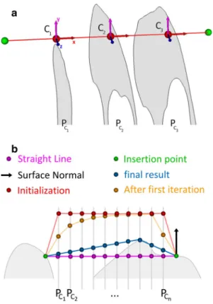
In this study, we were interested in generating the short-est path from the femoral insertion point to each of the two patellar insertion points, without penetrating any bone geometry. as described in [11], this can be achieved by introducing a set of n equally spaced control points Ci(xi,
yi, zi) connected by line segments. to this end, a local coor-dinate system is set up whose origin is located at the femo-ral insertion point and whose x-axis points to the patellar insertion point (see Fig. 1a). Based on this coordinate sys-tem, a plane PCi with origin Ci and normal vector parallel
to the local x-axis is defined for each point Ci. By doing so, the problem can be simplified to the calculation of the optimal position of Ci on PCi. to minimize the path length,
the sum of Euclidean distances between the control points has to be minimized:
Due to the equally spaced planes, the term xi+1 − xi is
constant and can be ignored during minimization.
the finer the resolution of control points, the better the path will adapt to the bone surface. However, a high num-ber of control points will increase the degrees of freedom of the optimization function, making the problem more dif-ficult to solve. We propose an iterative algorithm that will split the problem into local subtasks that can be solved in an efficient way.
2.1 Iterative path optimization
given a coarse initial solution, the key idea of the algorithm is to iterate through all control points and to locally opti-mize each point, assuming that all other points are optimal
(1) min Ci n i=0
(xi+1−xi)2+(yi+1−yi)2+(zi+1−zi)2
→min yi,zi n i=0 (yi+1−yi)2+(zi+1−zi)2
in the current state. a single control point Ci is defined as locally optimal if it is located on the straight non-penetrat-ing line connectnon-penetrat-ing Ci−1 and Ci+1. If the line penetrates the bone, Ci is instead defined as the closest non-penetrating point on PCi. any other choice of Ci will increase the length
of the path or will violate the non-penetration constraint. thus, the position of Ci will be updated in two steps. First,
the local optimum of the control point is determined with-out considering potential bone penetration. Since the con-trol points are distributed uniformly, the current optimal position can be simply calculated as the mean of the two neighboring points
note that the position of the predecessor Ct
i−1 has been
previously calculated within the same iteration t, while the successor Ct−1
i+1 still represents the position from the
previ-ous iteration. If the computed point is located inside the
Cti = 1 2
Ci−1t +Ci+1t−1 .
bone, the non-penetration constraint will be subsequently fulfilled by translating Ci to the closest bone surface point on plane PCi. to determine whether an updated control
point lies inside the bone, the outward pointing normal of the closest bone surface point on plane PCi can be used.
the computational expensive task for finding closest sur-face points on PCi can be performed efficiently by
effec-tively slicing the bone model into 2D contours for each plane using the so-called synchronized template algorithm of VtK [24]. Pre-calculation is possible since the planes are static throughout the optimization. By doing so, the closest point on a plane can be found efficiently using a KD-tree [1, 24]. In order to keep planes equally spaced, the control points were constrained to be moved only in the y- and z-direction of the coordinate system.
During the optimization process, the target func-tion decreases monotonically in each iterafunc-tion. If a point is not yet locally optimal, the total length of the path will decrease; otherwise the point will stay fixed, being
Fig. 1 Example depicting the path generation algorithm: the inser-tion points are shown in green, the initial soluinser-tion is depicted in red, and the result of the algorithm is denoted by the blue path. a First step the insertion points between femur and patella are connected by a straight line. the control points (denoted by C1, C2, C3) are initially defined as the intersection points between the straight line and the equally spaced planes PC1, PC2, PC3. the coordinate system is defined
such that the x-axis points from the femoral to the patellar insertion point. b Second step the initial solution (red) is created by moving each control point Ci (magenta) by 20 mm in direction of the surface
normal of the femoral insertion point (black arrow), in order to avoid bone collisions of the initial solution. thereafter, this initialization is optimized by iterating through the control points. the intermediate result after the first iteration is shown in orange and the final solution is depicted in blue. the bone surface is depicted by the gray-shaded region. c 3D case, demonstrating the progress of the algorithm from the initial solution (red) to the final result (blue). the planes PCi are
indicated by dark gray lines on the bone surface. View from proximal into the trochlea (top medial) (color figure online)
constrained by bone geometry. as a consequence, the global path length will decrease from iteration to itera-tion. therefore, the optimization process can be stopped if the length change between two consecutive iterations falls below a user-defined threshold. an example of the final optimization result is given in Fig. 1c. a rough ini-tial solution is needed, however, to avoid the algorithm to be trapped into a local minimum. an obvious choice would be the straight line between the insertion points. However, this initialization may not work in case of 3D models only representing the cortical bone layer (as in our case). Such models are hollow since cancellous bone and bone marrow were not segmented, which may cause the algorithm to fol-low the inner wall of the bone. therefore, the control points have to be moved away from the bone surface. to compute the direction of the offset, the bone surface normal at the femoral insertion point is projected on plane PCi.
thereaf-ter, each control point Ci is shifted by 20 mm in direction of the projected normal, as demonstrated in Fig. 1b, c. the iteration algorithm in pseudo code is described as follows:
2.2 Isometric score
a score was developed to quantify the isometry of the cho-sen insertion points for a subject. For a string s, the iso-metric score Is is defined as the sum of the relative mean squared errors (MSE) of the string lengths over all flexion positions. let P be the set of all flexion positions, lp,s be the length of string s in flexion position p, and ls the
aver-age length of the string over all flexion positions. then, the isometric score I of the graft is defined as the average of the isometric scores of both strings
where |P| denotes the number of measured flexion posi-tions. the score indicates the average relative length change during flexion, since the mean squared error is sensitive to the mean error as well as to the variance [13]. the higher the score becomes, the less isometric is the insertion point. For instance, given a string with an average length ls that is
1 % longer than ls in two positions and 1 % shorter in the
two other positions, the isometric score will be 0.1 × 10⁻³.
(2) Is∈{I,II}= 1 |P| p∈P lp,s−ls ls 2 I = II+III 2 , 2.3 Statistical analysis
the correlation between the isometric scores (i.e., I, I1, I2)
and the corresponding maximum length change was evalu-ated over all individuals using Pearson’s r. according to Eq. 2, the dependence between isometric score and length change can be expected to be quadratic. as Pearson’s r requires linear dependence, the maximum length has to be squared before calculation of the correlation coefficient. the calculation was performed using the software r (r Foundation, Vienna, austria).
3 Results
the graft consisting of two strings, namely string I and string II, was generated for each of the 10 subjects in all 4 flexion positions using the described method (see Fig. 2a). three different resolutions were analyzed to study their influence on the string length. In low,
medium, and high resolution, the strings were initial-ized with control points sampled at 4.5, 1.5, and 0.8 mm steps, respectively. thus, a string of 60 mm length gen-erated in medium resolution consisted of approximately 40 control points. the resolutions were chosen to be greater than the data resolution of 0.4 mm. In all reso-lutions, path refinement was performed until the length difference of a string between two iterations fell below 10−6 mm.
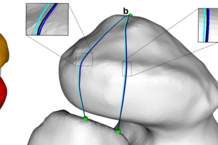
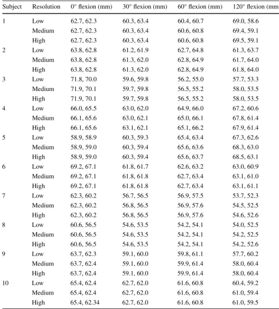
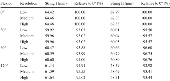
table 1 reports the string lengths during knee motion with respect to the different resolutions. In 11.25 %, the measured lengths changed considerably (i.e., more than Ct resolution) from low to medium resolution (maximum change 0.96 mm). Contrary, no length change greater than Ct resolution was observed from medium to high resolu-tion (maximum change 0.2 mm). table 2 shows the string lengths in the different flexion positions, averaged over all subjects. the average length of both strings was maximal in full extension (string I: 64.5 mm and string II: 62.8 mm). For string I, it was minimal in 30° of flexion (60.0 mm) and for string II in 120° of flexion (58.7 mm). the slightly differing paths resulting from the different resolutions are shown in Fig. 2b.
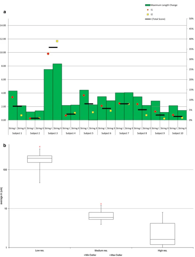
Figure 3a shows the isometric score of each subject, compared with the maximum relative length change dur-ing the entire range of motion. the correlation of all scores, i.e., I1, I2, and the combined score I, with the maxi-mum length change was above 0.99 (Pearson, P ≪ 0.01). In 9 of 10 subjects, the score was between 0.3 × 10⁻³
and 2.4 × 10⁻³. For subject 3, the score was greater than
10 × 10−3 in all resolution. In 80 % of the subjects, a
small average decrease of 6.2 % was measured from low to high resolution. Between these resolutions, the maximum decrease of 15.8 % was observed in subject 10 and the maximum increase of 19.8 % in subject 5.
For accuracy evaluation, two quality measures were introduced as depicted in Fig. 4a, b. Measure δ1 quantified the difference between a string and the actual bone surface in case of penetration. It was defined as the maximum pen-etration depth per line segment, averaged over all segments of a string. as shown in Fig. 4a, the penetration depth per segment was determined by sampling the line between two control points in 10 % steps with respect to the segment length. Complementary, δ2 measured the accuracy for the parts of a string that are not deformed by the bone surface. In these areas, the string should ideally follow a straight line. However, iterative algorithms have the characteristics to converge toward a solution and, dependent on the ini-tialization, they may never reach it exactly. In our case, this residual error is expressed by measure δ2, representing the
length difference between the non-penetrating part of the string and the corresponding straight line (i.e., ideal solu-tion) as depicted in Fig. 4b.
Figure 3b shows the distribution of δ1 among all 10
subjects. the average value of δ1 was 97.41 ± 120.49 µm (maximum: 620.51 µm) in low resolution, 3.55 ± 2.65 µm (maximum: 13.49 µm) in medium resolution, and 1.48 ± 1.42 µm (maximum: 5.67 µm) in high resolution. thus, δ1 decreased by 96.4 % between low and medium resolution and by 58.3 % between medium and high reso-lution. a similar pattern can be observed for the maximal
penetration depth of the strings. In low resolution, the max-imum penetration depth ranged from 0.27 to 2.4 mm (aver-age: 1.0 mm), in medium and high resolution from 0.016 to 0.094 mm (average: 0.043 mm), and 0.003 to 0.033 mm (average: 0.015 mm), respectively. a maximum penetration depth greater than the Ct resolution was only measured in low resolution (in 9 of the 10 subjects).
Besides accuracy evaluation, two additional experiments were carried out. First, the target function of Eq. 1 was solved with a general-purpose numerical optimizer (i.e., Powell’s nonlinear constrained optimization [21]). While the generated string was detoured by the bone geometry prop-erly, it did not always converge to a straight line between the bones, as demonstrated in Fig. 5. this characteristics was also expressed by measure δ2. While the error measure was
high when using Powell’s method (δ2 > 2 %), it was below 0.16 % for all subjects and resolutions with our algorithm. Secondly, an experiment was performed to examine the robustness of the proposed algorithm in case of different ini-tial solutions. thirty iniini-tializations were generated for each of three selected subjects. the initializations were generated by rotating the surface normal vector, which would be nor-mally used to create the initial solution, by a random value of up to 70°. In all experiments, the recomputed path was either equal to our result or it converged to a different local mini-mum which, however, always resulted in a longer path.
the calculation time needed to generate a single string did primarily depend on the desired resolution. On average, the generation using a mobile Intel Core [email protected] gHz, 10 gB memory took 0.9 ± 0.7 s in low resolution, 11.3 ± 5.6 s in medium resolution, and 32.9 ± 16.4 s in high resolution.
4 Discussion
In this study, we have investigated in vivo length changes between femoral–patellar graft insertion points using a
Fig. 2 a 3D strings (blue) generated by the proposed algorithm, depicted in each of the four flexion positions from 0° (yellow) to 120° (violet). the control points were sampled in medium resolution. View from distal/medial (top proximal, left medial). b Comparison of the strings in different resolutions: cyan, blue, and dark blue denote the string in low, medium, and high resolution, respectively. View from distal into the intercondylar notch (top medial) (color figure online)
custom-made algorithm for path generation. Similar meth-ods were described previously for estimating 3D length changes of ligaments in the knee [9, 27, 28] and for other anatomy [5, 11, 14, 15, 19].
the most straight forward way for quantifying length changes during motion is to measure the direct distance between insertion points as described in a study of Zhu et al. [28], analyzing length changes of the tibia-patellar ligament during flexion.
However, the method of Zhu et al. ignores possible intersection between the bone surfaces and the direct con-nection of the intersection points. Kobayashi et al. [9] described a technique in which intersecting paths were manually refined. they performed an MrI-based study for investigating the tibia-patellar tendon kinematics dur-ing a weight-beardur-ing deep knee bend in 6 different flexion positions. the patellar ligaments were modeled as manu-ally constructed lines connecting the insertion points on the
patella and the femur. If a line intersected the bone surface, it was manually split into two new line segments being tan-gential to the bone surface. In their study, high penetration depths of up to 2.1 ± 2.0 mm were observed. the penetra-tion depth error using our algorithm was of similar magni-tude in low resolution (average 1.0 mm), but considerably lower in medium resolution (0.04 mm on average). Increas-ing the path accuracy in the method of Kobayashi et al. would require iterative splitting and subsequent refinement of the line segments in a manual fashion, which can be very time-consuming.
as a consequence, an automatic method was proposed by Marai et al. to facilitate this task [5, 11]. their algo-rithm permitted to estimate ligament lengths of the distal radioulnar joint by automatically calculating the short-est non-penetrating path between insertion points. More recently, their technique was also applied for measuring length changes of the interosseous membrane [15], the
Table 1 the length of the computed graft, consisting of the two virtual strings (I and II), given for each subject and flexion position
In low, medium, and high resolution, the number of control points per string was between 10–13, 31–37, and 46–76, respectively
Subject resolution 0° flexion (mm) 30° flexion (mm) 60° flexion (mm) 120° flexion (mm)
1 low 62.7, 62.3 60.3, 63.4 60.4, 60.7 69.0, 58.6 Medium 62.7, 62.3 60.3, 63.4 60.6, 60.8 69.4, 59.1 High 62.7, 62.3 60.3, 63.4 60.6, 60.8 69.5, 59.1 2 low 63.8, 62.8 61.2, 61.9 62.7, 64.8 61.3, 63.7 Medium 63.8, 62.8 61.3, 62.0 62.8, 64.9 61.7, 64.0 High 63.8, 62.8 61.3, 62.0 62.8, 64.9 61.8, 64.0 3 low 71.8, 70.0 59.6, 59.8 56.2, 55.0 57.7, 53.3 Medium 71.9, 70.1 59.7, 59.8 56.5, 55.2 58.0, 53.5 High 71.9, 70.1 59.7, 59.8 56.5, 55.2 58.0, 53.5 4 low 66.0, 65.5 63.0, 62.0 64.9, 66.0 67.2, 60.6 Medium 66.1, 65.6 63.0, 62.1 65.0, 66.1 67.8, 61.4 High 66.1, 65.6 63.1, 62.1 65.1, 66.2 67.9, 61.4 5 low 58.9, 58.9 60.3, 59.3 65.4, 63.4 67.3, 62.6 Medium 58.9, 59.0 60.3, 59.4 65.6, 63.6 68.3, 63.0 High 58.9, 59.0 60.3, 59.4 65.6, 63.7 68.5, 63.1 6 low 69.2, 67.1 61.8, 61.7 62.6, 63.2 63.0, 60.9 Medium 69.2, 67.1 61.8, 61.8 62.7, 63.4 63.1, 61.0 High 69.2, 67.1 61.8, 61.8 62.7, 63.4 63.1, 61.1 7 low 62.3, 60.2 56.7, 56.5 56.9, 57.5 53.7, 52.3 Medium 62.3, 60.2 56.8, 56.5 56.9, 57.6 54.5, 52.5 High 62.3, 60.2 56.8, 56.5 56.9, 57.6 54.6, 52.6 8 low 60.6, 56.5 54.6, 53.5 54.2, 54.1 54.0, 52.5 Medium 60.6, 56.5 54.6, 53.5 54.2, 54.1 54.2, 52.5 High 60.6, 56.5 54.6, 53.5 54.2, 54.1 54.2, 52.6 9 low 63.7, 62.3 59.1, 60.0 59.8, 61.1 57.7, 60.2 Medium 63.7, 62.4 59.1, 60.0 59.9, 61.4 58.0, 60.4 High 63.7, 62.4 59.1, 60.0 59.9, 61.4 58.0, 60.4 10 low 65.4, 62.4 62.7, 62.0 61.6, 60.8 60.4, 59.2 Medium 65.4, 62.4 62.7, 62.0 61.6, 60.8 61.0, 59.4 High 65.4, 62.34 62.7, 62.0 61.6, 60.8 61.0, 59.5
ulnocarpal ligaments [14], and the radioulnar ligaments [19]. However, the algorithm of Marai et al. requires the calculation of a high-resolution distance map representa-tion of the bones. as a consequence, complex preprocess-ing must be performed before path generation. a smooth parameterized bone geometry has to be reconstructed by fitting a manifold surface to a 3D point cloud of the bone. thereafter, the distance map can be computed by sam-pling the parametric model. In contrast to their method, our algorithm can be directly applied to standard 3D sur-face models, considerably simplifying the entire work-flow. additionally, the use of a distance map has also several technical limitations such as high memory con-sumption and small inaccuracies as stated by the authors themselves [11].
Closely related to our work is the study of Yoo et al. [27] who was one of the first investigating in vivo length changes of the MPFl using a similar computer-based method. Ct data of 10 healthy subjects were used to reconstruct 3D knee models in five different flexion posi-tions. Virtual line segments were constructed along the 3D surface of the bones to estimate the reconstructed MPFl using commercial software. a difference to our approach is that they applied their technique on models based on non-weight-bearing knees. additionally, the validity of their path generation procedure was not demonstrated since neither technical details nor an accuracy evaluation was given.
In contrast to Yoo et al., we demonstrated quantitatively that the characteristics of the strings generated with our method were as intended: the path was detoured by bony protrusions to avoid penetration (δ1 < 0.01 mm in medium resolution); otherwise it followed a straight line as closely as possible (δ2 < 0. % in medium resolution). the results indicated that high resolution did not result in less penetra-tion compared with medium resolupenetra-tion. Contrary, in low
resolution, the generated path penetrated the bone surface considerably deeper than Ct resolution (maximum δ1:
0.6 mm, maximum penetration depth: 2.4 mm). the string length was already sufficiently estimated in low resolution for most of the cases, since the relative length change from low to medium resolution was smaller than 0.1 %. Besides accuracy of the generation, the measured length is also dependent on the quality of the bone geometry. a goal of the study was to employ the most accurate imaging tech-nology for the acquisition of bone anatomy. nonetheless, the segmentation process may introduce additional errors. In [18], Oka et al. performed an accuracy evaluation of long-bone segmentation, based on Ct data having a slice thickness of 1 mm. In their study, an average segmentation error of 0.45 mm was measured using the same segmenta-tion software and techniques as in our work. Based on these findings, a segmentation error of half the Ct slice thickness must be taken into account as well.
Smirk et al. [25] considered an insertion point as iso-metric if the total length variation during flexion was below 5 mm for string lengths between 47.2 and 70 mm. the isometric score proposed in our study has the advan-tage that it incorporates the length changes of all flexion positions. to allow comparison with the measure of Smirk et al., one can assume a ligament with an average length of 70 mm that is 2.5 mm longer than the average in two flexion positions and 2.5 mm shorter in the other two positions, resulting in an isometric score of 1.25 × 10⁻³
according to Eq. 2. Using this limit, 40 % of the defined femoral insertion points can be considered as isometric throughout the entire range of motion. this agrees with the study of Yoo et al. [27], who also identified the fem-oral adductor tubercle to be an isometric insertion point. a reason why the chosen point was not isometric in the remaining subjects of our study may be that definition of the point was only based on bony landmarks without
Table 2 the average length of the computed graft over all subjects, given for each string and flexion position
Flexion resolution String I (mm) relative to 0° (%) String II (mm) relative to 0° (%)
0° low 64.42 100.00 62.79 100.00 Medium 64.46 100.00 62.83 100.00 High 64.46 100.00 62.83 100.00 30° low 59.92 93.03 60.01 95.56 Medium 59.96 93.02 60.04 95.57 High 59.96 93.02 60.05 95.57 60° low 60.47 93.88 60.66 96.60 Medium 60.59 93.99 60.79 96.75 High 60.60 94.00 60.80 96.76 120° low 61.14 94.91 58.39 92.98 Medium 61.59 95.55 58.69 93.41 High 61.64 95.62 58.71 93.44
considering potential subject-specific anatomical differ-ences. this assumption is further supported by the fact that the best location of the femoral graft insertion point is still
not clearly defined [20], although several studies [25–27] were performed to determine the most isometric point among several candidate points.
Fig. 3 a the isometric score I in comparison with the maximum length change (in percent; right scale) during flexion, given for each subject. I1 and I2 denote the isometric score of string I and string II,
respectively. I denotes the total isometric score for the given subjects (left scale). b tukey boxplot showing the distribution of δ1 among all subjects, given for each resolution
Our findings agreed with results of previous cadaver studies which investigated the MPFl length of the knee under loaded conditions [17, 26]. During flexion, we meas-ured an average length change of 7.2 and 5.6 mm for string I and string II, respectively. Steensen et al. [26] described an average length change of 7.9 and 4.5 mm using the same insertion points. In our experiments, the longest distance of string I was observed in 0° of flexion and the shortest dis-tance in 30° flexion on average. In the cadaver study per-formed by nomura et al. [17], the MPFl was very taught in 0° of flexion and relaxed in 30° of flexion when load was applied. Different results were reported in studies [25, 27] analyzing knees in a non-weight-bearing condition. Smirk and Morris [25] reported the smallest distance between the insertion points in full flexion; the greatest distance was observed between 30° and 60° of flexion. Yoo et al. [27] measured the smallest distance in full flexion for both strings, and the greatest distance for string I and string II in full extension and 30° flexion, respectively.
Our study has several limitations. First of all, a relatively small sample size of only 10 subjects was analyzed. How-ever, the study provided preliminary results on the MPFl path length under physiological loading conditions using high-resolution bone geometry and can, therefore, be con-sidered as a pilot study. Secondly, the graft was simpli-fied to two non-penetrating string between insertion points ignoring biomechanical and material properties (e.g., fiber directions and stiffness), thus representing a compromise between complex physically based simulation and simple approaches not considering penetration. lastly, the in vivo knee joint kinematic was only acquired in four flexion posi-tions which may be insufficient to fully cover the entire patellar motion.
In conclusion, the described methods appeared to be feasible for estimating the length of the MPFl in a normal knee, which enabled us to study isometric behavior. Since the algorithm solely relies on standard 3D bone models, the range of application is versatile. For instance, the method may be applied to 3D models obtained from magnetic res-onance tomography (Mrt) images, since this modality is frequently used in the pre-operative assessment of MPFl tear. the accuracy of the method if applied to different image modalities is subject of further research. Ultimately, the proposed approach may be used to find the optimal insertion point with respect to isometry and subject-specific anatomy in an automatic fashion which may give additional insights for the pre-operative planning of MPFl recon-struction. this important aspect will be addressed in future work as well.
Conflict of interest the authors declared that they have no conflicts of interests in the authorship and publication of this contribution. Fig. 4 Example demonstrating the calculation of δ1 and δ2. a δ1 is
defined as the averaged sum of maximum penetration depths per seg-ment. the arrows exemplarily denote the 10 % sampling of the line segment. b Calculation of δ2: Floating points (light blue) are defined as points not lying on or inside of the bone. Bone detachment points (violet) are the end points of consecutive line segments, consisting only of floating points. δ2 is defined as the length difference between the generated path (blue line) and the straight line (dashed violet line), relative to the total length of the string (color figure online)
Fig. 5 general-purpose numerical optimizers, such as Powell’s non-linear constrained optimization [21], generate paths which sometimes fail to converge to the desired solutions (depicted in magenta). the solution of our algorithm is shown in blue. View from distal into the intercondylar notch (top medial) (color figure online)
References
1. Bentley Jl (1975) Multidimensional binary search trees used for associative searching. Commun aCM 18(9):509–517
2. Besl PJ, McKay nD (1992) a method for registration of 3-D shapes. Pattern anal Mach Intell IEEE trans 14(2):239–256 3. Bollier M, Fulkerson J, Cosgarea a, tanaka M (2011) technical
failure of medial patellofemoral ligament reconstruction. arthros-copy 27(8):1153–1159
4. Burks rt, Desio SM, Bachus Kn, tyson l, Springer K (1998) Biomechanical evaluation of lateral patellar dislocations. am J Knee Surg 11(1):24–31
5. Crisco JJ, Moore DC, Marai gE, laidlaw DH, akelman E, Weiss aP et al (2007) Effects of distal radius malunion on dis-tal radioulnar joint mechanics—an in vivo study. J Orthop res 25(4):547–555
6. Deie M, Ochi M, Sumen Y, Yasumoto M, Kobayashi K, Kimura H (2003) reconstruction of the medial patellofemoral ligament for the treatment of habitual or recurrent dislocation of the patella in children. J Bone Joint Surg Br 85(6):887–890
7. Desio SM, Burks rt, Bachus Kn (1998) Soft tissue restraints to lateral patellar translation in the human knee. am J Sports Med 26(1):59–65
8. Hautamaa PV, Fithian DC, Kaufman Kr, Daniel DM, Pohlmeyer aM (1998) Medial soft tissue restraints in lateral patellar instabil-ity and repair. Clin Orthop relat res 349:174–182
9. Kobayashi K, Sakamoto M, Hosseini a, rubash HE, li g (2012) In-vivo patellar tendon kinematics during weight-bearing deep knee flexion. J Orthop res 30(10):1596–1603
10. lorensen WE, Cline HE (1987) Marching cubes: a high resolu-tion 3D surface construcresolu-tion algorithm. SIggraPH Comput graph 21(4):163–169
11. Marai gE, laidlaw DH, Demiralp C, andrews S, grimm CM, Crisco JJ (2004) Estimating joint contact areas and ligament lengths from bone kinematics and surfaces. IEEE trans Biomed Eng 51(5):790–799
12. Matthews JJ, Schranz P (2010) reconstruction of the medial patellofemoral ligament using a longitudinal patellar tunnel tech-nique. Int Orthop 34(8):1321–1325
13. Montgomery DC, runger gC (2010) applied statistics and prob-ability for engineers. Wiley. ISBn: 9780470053041
14. Moritomo H, Murase t, arimitsu S, Oka K, Yoshikawa H, Suga-moto K (2008) Change in the length of the ulnocarpal ligaments during radiocarpal motion: possible impact on triangular fibrocar-tilage complex foveal tears. J Hand Surg am 33(8):1278–1286 15. Moritomo H, noda K, goto a, Murase t, Yoshikawa H,
Suga-moto K (2009) Interosseous membrane of the forearm: length change of ligaments during forearm rotation. J Hand Surg am 34(4):685–691
16. Mountney J, Senavongse W, amis aa, thomas nP (2005) ten-sile strength of the medial patellofemoral ligament before and after repair or reconstruction. J Bone Joint Surg Br 87(1):36–40 17. nomura E, Inoue M, Osada n (2005) anatomical analysis of
the medial patellofemoral ligament of the knee, especially the femoral attachment. Knee Surg Sports traumatol arthrosc 13(7):510–515
18. Oka K, Murase t, Moritomo H, goto a, Sugamoto K, Yoshikawa H (2009) accuracy analysis of three-dimensional bone surface models of the forearm constructed from multidetector computed tomography data. Int J Med robot 5(4):452–457
19. Omori S, Moritomo H, Murase t, Miyake J, Kataoka t, Kawani-shi Y et al (2013) Changes in length of the radioulnar ligament and distal oblique bundle after Colles’ fracture. J Plast Surg Hand Surg 47(5):409–414
20. Philippot r, Chouteau J, Wegrzyn J, testa r, Fessy MH, Moyen B (2009) Medial patellofemoral ligament anatomy: implica-tions for its surgical reconstruction. Knee Surg Sports traumatol arthrosc 17(5):475–479
21. Powell MJD (1994) a direct search optimization method that models the objective and constraint functions by linear interpola-tion. In: gomez S, Hennart J-P (eds) advances in optimization and numerical analysis. Mathematics and Its applications, vol 275. Springer, netherlands, pp 51–67
22. Schottle PB, Fucentese SF, romero J (2005) Clinical and radio-logical outcome of medial patellofemoral ligament reconstruction with a semitendinosus autograft for patella instability. Knee Surg Sports traumatol arthrosc 13(7):516–521
23. Schottle PB, Schmeling a, rosenstiel n, Weiler a (2007) radi-ographic landmarks for femoral tunnel placement in medial patellofemoral ligament reconstruction. am J Sports Med 35(5):801–804
24. Schroeder W, Martin K, lorensen B (2006) Visualization toolkit: an object-oriented approach to 3D graphics, 4th edn. Kitware, ISBn: 193093419X
25. Smirk C, Morris H (2003) the anatomy and reconstruction of the medial patellofemoral ligament. Knee 10(3):221–227
26. Steensen rn, Dopirak rM, McDonald Wg 3rd (2004) the anat-omy and isometry of the medial patellofemoral ligament: impli-cations for reconstruction. am J Sports Med 32(6):1509–1513 27. Yoo YS, Chang Hg, Seo YJ, Byun JC, lee gK, Im H et al (2012)
Changes in the length of the medial patellofemoral ligament: an in vivo analysis using 3-dimensional computed tomography. am J Sports Med 40(9):2142–2148
28. Zhu Z, Ding H, Dang X, tang J, Zhou Y, Wang g (2010) In vitro kinematic measurements of the patellar tendon in two different types of posterior-stabilized total knee arthroplasties. Conf Proc IEEE Eng Med Biol Soc 2010:3938–3941
![Fig. 5 general-purpose numerical optimizers, such as Powell’s non- non-linear constrained optimization [21], generate paths which sometimes fail to converge to the desired solutions (depicted in magenta)](https://thumb-eu.123doks.com/thumbv2/123doknet/14814167.612774/9.892.107.402.706.952/numerical-optimizers-constrained-optimization-generate-converge-solutions-depicted.webp)