DOI 10.1007/s00348-014-1849-7 RESEARCH ARTICLE
Mind the gap: a new insight into the tip leakage vortex using
stereo‑PIV
Matthieu Dreyer · Jean Decaix · Cécile Münch‑Alligné · Mohamed Farhat
Received: 21 August 2014 / Revised: 10 October 2014 / Accepted: 23 October 2014 / Published online: 5 November 2014 © Springer-Verlag Berlin Heidelberg 2014
of a specific tip clearance for which the vortex strength is maximum and most prone to generating cavitation.
List of symbols
c Hydrofoil chord
h Maximum foil thickness
W∞ Inlet velocity p∞ Inlet pressure x, y, z Cartesian coordinates
u, v, w Spanwise, transverse and axial velocity xc, yc Vortex center coordinates
rc Vortex core radius
Rec Reynolds number (W∞c/ν)
α Incidence angle
τ Normalized tip clearance (gap/h)
ω Vorticity
Γ Circulation
Γ∗ Normalized circulation (Γ /W∞rc)
Γ∞∗ Γ∗ at τ = 2
Cpmin Pressure coefficient in the vortex center
p(r = 0) − p∞ 1 2ρW∞2 1 Introduction
Tip vortices are prevalent in many industrial applications (e.g., air transportation, marine propulsion, wind turbines, hydraulic machines, space rockets). The need to understand and control the dynamics of these flows has driven numer-ous researches, producing an abundant literature [see Green (1995) and Arndt (2002) for a review]. From a theoretical point of view, the model of Batchelor (1964), valid far down-stream of the wing tip, is widely used to describe the struc-ture of the trailing vortex flow. Moore and Saffman (1973)
Abstract The tip leakage vortex (TLV), which
devel-ops in the clearance between the rotor and the stator of axial hydro turbines, has been studied for decades. Yet, many associated phenomena are still not understood. For instance, it remains unclear how the clearance size is related to the occurrence of cavitation in the vortex, which can lead to severe erosion. Experiments are here carried out on the influence of the clearance size on the tip vortex structure in a simplified case study. A NACA0009 hydro-foil is used as a generic blade in a water tunnel while the clearance between the blade tip and the wall is varied. The 3D velocity fields are measured using Stereo Particle Image Velocimetry (SPIV) in three planes located downstream of the hydrofoil for different values of the upstream velocity, the incidence angle and a large number of tip clearances. The influence of the flow conditions on the structure of the TLV is described through changes in the vortex inten-sity, core axial flow, vortex center position and wandering motion amplitude. Moreover, high-speed visualizations are used to highlight the vortex core trajectory and clearance flow alteration, turning into a wall jet as the tip clearance is reduced. The measurements clearly reveal the existence
Electronic supplementary material The online version of this article (doi:10.1007/s00348-014-1849-7) contains supplementary material, which is available to authorized users.
M. Dreyer (*) · M. Farhat
Laboratory for Hydraulic Machines, Ecole polytechnique fédérale de Lausanne, Av. de Cour 33 bis,
1007 Lausanne, Switzerland e-mail: [email protected] J. Decaix · C. Münch-Alligné
Institut Systèmes industriels, HES-SO Valais-Wallis, Route du Rawyl 47, 1950 Sion, Switzerland
developed a more sophisticated model, valid in the interme-diate region between the completion of roll-up and the far field, where the Batchelor solution holds. Recently, Pino et al. (2011) used SPIV to measure the 3D velocity field in the tip vortex behind a foil. Better agreement with the model of Moore and Saffman than that of Batchelor was observed. In axial turbomachinery, a leakage flow occurs between the blade tip and the casing, driven by the pressure difference between the blade pressure and suction sides. The vorticity shed by this leakage flow rolls up into the so-called tip leak-age vortex (TLV), which is strongly influenced by the vicin-ity of the wall (confinement). In axial hydraulic machines, cavitation may develop in the core of TLVs, leading some-times to severe erosion of the runner blades and the casing, as well as an increase in structural vibrations. Farrell and Bil-let (1994) have found that cavitation incipience in an axial pump may be delayed if the tip clearance is set to an opti-mum value of about 0.2 times the maxiopti-mum blade thickness. Boulon et al. (1999) examined the effect of the clearance size on the tip vortex generated by an elliptical foil in a setup without relative motion between the end wall and the foil. They found, conversely, that the cavitation inception index increases as the gap is reduced, while no tip vortex cavitation was observed in the most confined cases. Similar observa-tions were reported by Gopalan et al. (2002) for the case of a cambered hydrofoil in a water tunnel. More recently, Wu et al. (2011) and Miorini et al. (2012) studied experimentally the internal structure of the TLV within the rotor of an axial waterjet pump using both 2D and stereo-PIV. They observed that the instantaneous TLV structure is composed of unsteady vortex filaments that propagate into the tip region of the blade passage and roll up into the TLV. They noticed that vortex breakdown could also occur as the TLV migrated toward the pressure side of the neighboring blade, changing drastically the vortex characteristics, as reported by Pasche et al. (2014). The measured velocity fields in these studies were, however, limited to a few tip clearance values.
In the specific area of Kaplan turbines, the wake of the distributor guide vanes produces a highly non-uniform pressure field, which leads to repetitive collapses and rebounds of the cavitating tip vortices. Obviously, cavita-tion erosion depends not only on the vortex strength and core size, but also on its trajectory and how far it stands from solid boundaries. It should be noted that, nowadays, it is still not possible to fairly predict cavitation occurrence in axial turbines, neither from numerical simulations nor from reduced scale model tests. In their attempt to mitigate the cavitation development in axial turbines, engineers com-monly implement the so-called anti-cavitation lip, which consist of a simple winglet attached to the tip of the blades. Nevertheless, such a remedy often fails to reduce cavita-tion erosion, as reported by Roussopoulos and Monkewitz (2000) on a simplified case study.
In the present study, the structure and trajectory of a TLV generated at the tip of a fixed 2D hydrofoil are inves-tigated experimentally for different confinements and flow parameters. Our objective is to perform accurate measure-ments of the velocity field to better understand the under-lying physics of vortex confinement and provide an exten-sive experimental database for further developments. In our simplified approach, the effect of relative motion between the rotating blades and the casing of an axial turbine is not taken into account. It is assumed that the mean vortex flow is not fundamentally altered by the end wall motion, as already shown by Wang and Devenport (2004).
It is well known that velocity measurements in vortical structures are subjected to uncertainty due to the wandering phenomenon, which is a random displacement of the vor-tex centerline with amplitude of the order of the vorvor-tex core size. Although this phenomenon has been well referenced, its origin remains unclear. It is presumed to arise from a resonant excitation triggered by the free-stream turbulence (Fabre et al. 2008). As a consequence, single point measure-ment techniques, such as Laser Doppler Velocimetry (LDV), always result in a more diffuse velocity field than in real-ity, and correction methods must be applied to retrieve the true velocity field, cf. Devenport et al. (1996); Iungo et al. (2009); and Pasche et al. (2014). Furthermore, the finite size of the LDV measurement volume introduces another smoothing effect that must also be accounted for (Le Guen et al. 1997). Therefore, we have selected the SPIV tech-nique for the measurement of the 3D velocity field, since it leaves the possibility of accurately filtering out this wander-ing through various processwander-ing tools, as those proposed, for instance, by Bhagwat and Ramasamy (2012).
2 Experimental setup
2.1 Case study and setup
The experiments are carried out in the EPFL high-speed cavitation tunnel. The squared test section is 150 mm wide and 750 mm long. A honeycomb and a contraction nozzle (ratio 46:1) upstream of the test section ensure a low tur-bulence level (below 1 %). The maximum inlet flow veloc-ity is 50 m/s. The static pressure in the test section can be varied from near vacuum up to 10 bars. The operating flow parameters are the upstream velocity W∞, the pressure in the test section inlet p∞, and the hydrofoil incidence angle α. The test section walls are made of 80-mm-thick plexi-glass, providing a good optical access to the flow. The TLV is generated by a stainless steel NACA0009 hydrofoil with a thickness distribution yb given by Eq. (1), using c0 = 110 mm for the chord length. The foil is truncated at c = 100 mm, its span is 150 mm, and its maximum thickness h is
9.9 mm. The foil tip pressure side corner was rounded with a small radius of 1 mm in order to limit the cavitation in the clearance during the flow visualizations. It is mounted on a sliding support allowing for an adjustable clearance (or gap) between the foil tip and the test section lateral wall. The gap can be varied smoothly between 0 and 20 mm. The influence of the foil boundary-layer state is also investi-gated by testing smooth and roughened leading edge. The turbulent boundary-layer can be tripped with a 4-mm-wide strip of distributed roughness, made of glue and 125-μm-diameter sand. The roughness is placed on both sides of the hydrofoil, 4 mm downstream of the leading edge, as described by Ausoni et al. (2012).
The results are represented in the Cartesian x, y, z coor-dinate system. Its origin is located on the test section lat-eral wall, corresponding to the plane x = 0, while the foil axis of rotation is on the intersection of the planes y = 0 and z = 0. The orientation of the coordinate system is illus-trated in Fig. 1. (1) yb c0 = a0 � x c0 �1/2 + a1 � x c0 � + a2 � x c0 �2 + a3 � x c0 �3 0 ≤ x c0 ≤ 0.5 yb c0 = b0+ b1 � 1 −c0x � + b2 � 1 −c0x �2 + b3 � 1 −c0x �3 0.5 < x c0 ≤ 1.0 a0= +0.1737 b0= +0.0004 a1= −0.2422 b1= +0.1737 a2= +0.3046 b2= −0.1898 a3= −0.2657 b3= +0.0387 2.2 Flow investigations
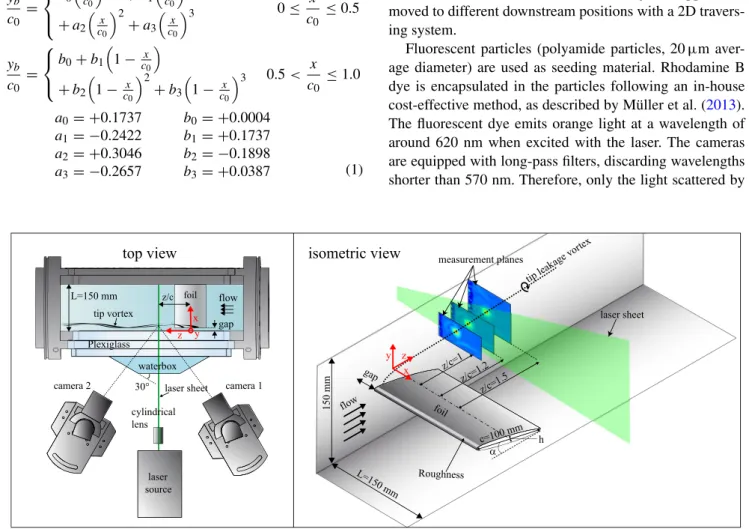
SPIV is used to measure the 3D velocity field in three cross-sections of the tip vortex at different downstream locations (see Fig. 1). A 2-mm-wide laser sheet is generated by a double-pulsed YAG laser (Litron DualPower, 200 mJ/ pulse, 532 nm wavelength) and a cylindrical lens. The time interval between laser pulses is set for each inlet velocity in order to limit the maximum out-of-plane displacement of the seeding particles to one-tenth of the laser sheet thick-ness (e.g., 30 µs for W∞= 5 m/s). Image pairs are acquired using two CCD cameras (Dantec FlowSense E0 4M) with a resolution of 2,048 × 2,048 pixels. The cameras are mounted on both sides of the laser sheet with an orienta-tion of 30° with respect to the latter. To minimize the opti-cal distortions, a transparent water box is mounted on the lateral wall. Its fixation is ensured by creating a partial vacuum, allowing for a simple positioning procedure. Two 60-mm lenses are used in combination with Scheimpflug mounts to align the focal plane with the laser sheet. The laser and the cameras are mounted on a joint support and moved to different downstream positions with a 2D travers-ing system.
Fluorescent particles (polyamide particles, 20 µm aver-age diameter) are used as seeding material. Rhodamine B dye is encapsulated in the particles following an in-house cost-effective method, as described by Müller et al. (2013). The fluorescent dye emits orange light at a wavelength of around 620 nm when excited with the laser. The cameras are equipped with long-pass filters, discarding wavelengths shorter than 570 nm. Therefore, only the light scattered by
measurement planes laser sheet gap 150 mm L=150 mm α tip leakage vortex isometric view z/c=1.5 foil c=100 mm z/c=1.2 z/c=1 h Roughness Plexiglass gap laser source cylindrical lens top view camera 1 camera 2 laser sheet
tip vortex waterbox 30° L=150 mm z/c foil x y z x z y flow flow
Fig. 1 Sketch of the SPIV configuration used in the 3D measurement of the velocity field. Left top view of the tunnel test section and optical instruments. Right isometric view of the inlet test section with the three measurement planes
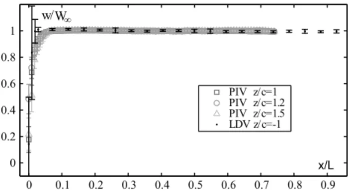
the particles is recorded. The out-of-plane velocity com-ponent is obtained by combining the 2D velocity fields derived for each camera. A third-order polynomial cali-bration ensures the conversion between the camera refer-ence frame and the real physical dimensions. To this end, a 100 × 100 mm double-faced doted target (dots separated by 2.5 mm) is immersed in the test section and is imaged at several positions within the width of the laser sheet. The accuracy of the calibration is verified by comparing the streamwise velocity profiles (corresponding to the out-of-plane component) measured by SPIV with that measured by LDV, see Fig. 2. Excellent agreement in the velocity data is observed. The large standard deviation in the wall boundary-layer measured by the LDV is due to the finite size of the control volume (about 1.2 mm) in a region of high velocity gradients.
Finally, cavitation in the TLV core is used as a tracer to follow the vortex trajectory. A high-speed camera (Pho-tron SA1.1) along with a xenon flash light (11-ms dura-tion and 1.1-KJ energy) is used to visualize the cavitating TLV dynamics at 20,000 frames per second for several flow regimes.
3 Analysis methodology
3.1 Flow parameters and PIV processing
The velocity field is measured in a cavitation-free regime at three streamwise positions (z/c = 1, 1.2 and 1.5) down-stream of the hydrofoil. At each position, five incidence angles (3◦, 5◦, 7◦, 10◦, 12◦) are tested in combination with up to four inlet velocities (5, 10, 15 and 20 m/s). The Reynolds number based on the foil chord Rec= W∞c/ν varies from 5 × 10⁵ to 2 × 10⁶. For each of these con-figurations, the tip clearance is varied between 0 and 20 mm. Moreover, measurements are performed both with
and without the turbulent boundary-layer tripping on the hydrofoil leading edge, yielding a total of 1,170 distinct configurations.
The velocity fields are derived by processing the acquired image pairs with an adaptive multi-pass correla-tion algorithm, which adjusts the size and shape of the individual Interrogation Areas (IAs) with the local seeding densities and flow gradients. The criterion for the IA size is the presence of at least eight particles and a minimum of 16 × 16 pixels. A total of 182 × 120 velocity vectors with a spatial resolution of 0.6 mm are finally obtained. The vec-tor fields are validated with a universal outlier test, and spu-rious vectors are replaced by the median value of the 5 × 5 neighboring vectors. The percentage of spurious vectors is around 5 %. The measurement errors are estimated assum-ing a 0.1 pixel uncertainty on the measurement of particle displacements (Westerweel 2000). Since both cameras con-tribute symmetrically to the measurements, the in-plane errors are smaller by a factor 1/√2 than the value for the single camera arrangement and the error of the out-of-plane component equals the in-plane error multiplied by 1/tan(φ) (Prasad 2000), where φ is the angle between the light sheet normal and the camera viewing direction. Given an aver-age particle displacement of 5 pixels, the uncertainties were estimated to 1.4 % for the in-plane components and 0.8 % for the out-of plane component. This is in accord-ance with Fig. 2 which gives <1 % error for the out-of-plane component. The average velocity field is determined after processing 100 individual vector fields for each operating condition. It is verified that increasing this number does not affect the mean flow characteristics.
The streamwise vorticity ω = ∂v/∂x − ∂u/∂y is com-puted by the numerical differentiation of the velocity field. To minimize bias errors and avoid any undesirable effect of the differentiation of a noisy field, the spatial sampling resolution is increased via a least-square cubic spline inter-polation of the velocity. The derivatives are then estimated with the following fourth-order Richardson numerical scheme:
3.2 Wandering correction
Wandering is a random fluctuation of the vortex axis with an amplitude comparable to the vortex core size. If not cor-rected, the wandering would yield to a larger core size and a lower value of the maximum velocity in the mean vortex flow, as mentioned previously.
(2) ωi,j=
1
12�X(−vi+2,j+ 8vi+1,j− 8vi−1,j+ vi−2,j)
− 1 12�Y(−ui,j+2+ 8ui,j+1− 8ui,j−1+ ui,j−2) 0 0.1 0.2 0.3 0.4 0.5 0.6 0.7 0.8 0.9 PIV z/c=1 PIV z/c=1.2 PIV z/c=1.5 LDV z/c=-1 0 0.2 0.4 0.6 0.8 1 w/W∞ x/L
Fig. 2 Comparison of the axial velocity profiles in the test section measured by PIV and LDV. No hydrofoil is mounted in the test sec-tion
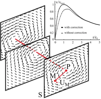
Several techniques are available to retrieve the swirl center such as the local partial orthogonal decomposi-tion used by Bouillot et al. (2014). In our case, we have implemented the algorithm of Graftieaux et al. (2001) to identify the vortex center and align the velocity maps before averaging, as illustrated in Fig. 3. Introducing the dimensionless scalar function Π at the position P, defined as:
where S is a rectangular domain of fixed size centered on P, M lies in S, z is the unit vector normal to the measure-ment plane, UM is the velocity vector and N is the
num-ber of velocity vectors inside S, as specified in Fig. 3. The function Π reaches a maximum equal to one at the location of the vortex center if the vortex is axisymmet-ric, but it would be lower for an asymmetrical vortex. Graftieaux’s algorithm is a simple yet highly robust way to identify the swirl center location of a velocity field. Unlike gradient-based vortex detection techniques, which are susceptible to experimental noise, Π does not require any gradient evaluation and considers only the topology of the velocity field. In general, the vortex center does not lie on a measurement grid node, and the realignment requires an interpolation of the measurement data. This is realized via the cubic spline interpolation of the velocity field mentioned previously.
(3) Π (P) = N1
S
(PM ∧ UM) · z
�PM� · �UM�
3.3 Identification of the key vortex parameters
Tip vortices are characterized by two zones: the core, close to the center of rotation where the viscous effects are dominant, and an outer region where the motion is mainly irrotational. This behavior can be modeled using simple vortex models such as that of Rankine and Lamb-Oseen. Vatistas et al. (1991) proposed a simplified expres-sion that encompasses a series of tangential velocity pro-files for a vortex structure, which can be written in the form:
The Vatistas model is used here, since by varying the shape parameter n in Eq. (4), a wide range of velocity profiles can be defined. When n = 1, the Scully vortex is reproduced, the case n ≈ 2 gives a close approximation to the Lamb-Oseen model, while n → ∞ corresponds to the Rankine vortex (Bhagwat and Leishman 2002). The minimum pres-sure coefficient in the vortex center can be derived by inte-grating the equilibrium equation ∂p/∂r = ρv2
θ/r, leading to the following expression of the minimum pressure coeffi-cient in the vortex center:
where β is a constant whose value depends on the choice of vortex model. For the Vatistas model, β is a function of the shape parameter n, as illustrated in Fig. 4, defined by:
Notice that Ŵ(n) denotes the Euler integral of the second kind (Gamma function), not to be confused with the cir-culation Γ . Equation (5) shows that the prediction of the minimum pressure in the vortex center effectively reduces to the estimation of two key parameters, namely the vortex circulation, Γ , and the viscous core radius, rc. The circu-lation is calculated by integrating the vorticity within the
(4) vθ(r) = Γ 2π r (r2n c + r2n)1/n (5) Cpmin = −β Γ W∞rc 2 (6) β(n) = 1 4π2 Ŵ(1 + 1/n)Ŵ(1/n) Ŵ(2/n) 0 1 2 3 4 5 0 0.2 0.4 0.6 0.8 1 r/rc v/vmax with correction without correction
S
M
P
U
M
Fig. 3 Left correction of the wandering by aligning all the vortex centers before averaging. Top right example of the wandering effect on the circumferential velocity
0 1 2 3 4 5 6 7 8 9 10 0 0.01 0.02 0.03 0.04 0.05 0.06 n Vatistas, β(n) =4π12Γ(1+1/n) Γ(1/n)(2/n) Lamb-Oseen, β ≈ 0.044 β Rankine, β =2π12 Γ
Fig. 4 Value of β in Eq. (5). The curve β(n) for the Vatistas model is plotted along with the Rankine and Lamb-Oseen β value
vortex core, the radius of which rc is estimated by a best fit—in least-squares sense—of the Vatistas model with
n = 2 over the measured velocity profiles.
4 Results and discussion
4.1 Flow visualizations
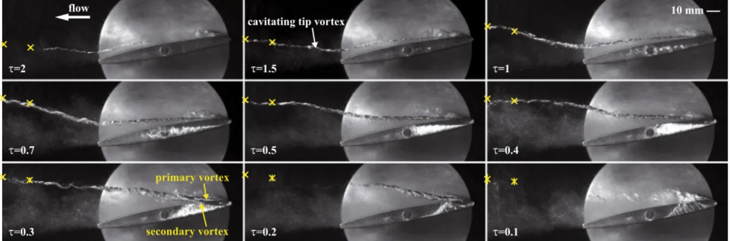
Cavitation can be a convenient way to visualize the tra-jectory of vortices, as reported by Chang et al. (2007). A reduction in the static pressure in the test section leads to the vaporization of the vortex core, which makes it visible. However, this is not a strictly passive means of flow visu-alization, as vapor can completely fill the vortex core, lead-ing to vorticity redistribution and possible alterations of the flow dynamics. Figure 5 presents high-speed visualization snapshots of the cavitating TLV for different values of tip clearance. The inlet velocity is 10 m/s, the incidence angle is 10◦, and p
∞ is kept to 1 bar for all clearances. To assess the mean TLV trajectory, we have summed the images cap-tured during 11 ms at 20,000 FPS. The result is given in Fig. 6 for three tip clearances. The scatter of the cavitation bubbles in the vortex core unveils the wandering amplitude which is quite small in theses cases. Moreover, comparisons
with the TLV position in cavitation-free regime, obtained by SPIV and represented by the yellow crosses in Figs. 5
and 6, indicate that neither the vortex trajectory nor the wandering amplitude are altered by the cavitation.
The trajectory of the TLV strongly depends on the clear-ance size: the smaller the gap, the more the vortex is pulled away from the hydrofoil. This is due to a purely potential flow effect and can be understood through the considera-tion of a simple model consisting of a 2D vortex above a wall, as explained by Doligalski et al. (1994). To ensure zero flow across the wall, an image vortex is placed sym-metrically to the actual TLV with respect to the confine-ment wall. This image vortex induces an upward velocity in the actual vortex, tending to move it upwards.
Another feature is the change in slope of the vortex trajectory at the foil trailing edge. This is particularly vis-ible if the TLV remains relatively close to the foil along the chord, i.e., at large clearances values like τ = 2. This phenomenon can again be explained with reference to the image system of the tip clearance flow. Over the foil, one must consider three images of the TLV to satisfy the rel-evant kinematic constraints, as reported by Chen et al. (1991). Two of the image vortices induce vertical veloci-ties on the actual vortex that partially cancel out. After the blade, there is only one image vortex needed to satisfy the
τ=1
τ=0.7 τ=0.5 τ=0.4
flow
τ=2 τ=1.5
cavitating tip vortex
τ=0.2
τ=0.3 τ=0.1
10 mm
primary vortex secondary vortex
Fig. 5 Snapshots of the cavitating TLV generated by a NACA0009 for different gap widths. The tip clearance is viewed from the side and is facing the observer. The yellow crosses represent the position
measured by SPIV in cavitation-free regime, in the planes z/c = 1 and 1.2. Flow conditions: W∞= 10 m/s, incidence = 10◦, p
∞= 1 bar.
The original movies are provided as supplementary material
τ=0.3
τ=1 τ=0.5
Fig. 6 Superposition of the cavitating TLV visualizations during 11 ms for three gap widths. The yellow crosses represent the position measured by SPIV in cavitation-free regime, in the planes z/c = 1 and 1.2. Flow conditions: W∞= 10 m/s, incidence = 10◦, p∞= 1 bar
boundary conditions, and the resulting induced upward velocity is thus larger.
The amount of cavitation in the vortex core reveals the changes of the vortex strength along the chord. As the clearance is reduced, the cavitation becomes more intense, but the vortex also become less coherent. For the most confined configuration, the vortex rapidly loses its coher-ence until practically vanishing. Cavitation in the clearance region also appears when the gap is reduced. This results from boundary-layer separation in the gap and can be reduced when the edge of the foil pressure side is rounded, as explained by Laborde et al. (1997). Clearance cavitation indicates that the gap flow turns into a vertical wall jet as the gap is reduced, entraining vorticity filaments into the TLV. It also reveals that the TLV results from the merging of a primary vortex, originating at the leading edge, and a secondary vortex that develops in the clearance (visible in the cases τ = 0.3 and 0.2, see also the movies provided as supplementary material). In fact, flow visualizations at low inlet pressure showed that the secondary vortex exists for all clearances. However, as it is weaker than the primary vortex, the secondary vortex is not visible on Fig. 5 for large clearances. The secondary and primary vortices sys-tematically merge together, and the merging location moves toward the foil leading edge as the clearance is reduced. 4.2 TLV characteristics
The TLV is formed by the rolling up of the vorticity trans-ported by the leakage flow which is driven by the pressure gradient across the clearance. Its characteristics depend on the operating conditions, such as the foil incidence angle, the inlet velocity and the wall proximity. Figure 7 illustrates the influence of the hydrofoil incidence on the TLV for a fixed normalized clearance τ = 1.5. Vorticity maps with 2D streamlines are represented for two incidences, 5◦ and 12◦, while the evolution of the vortex circulation Γ with the incidence is plotted below for the smooth and rough foil. The vorticity is concentrated in a small volume correspond-ing to the vortex viscous core while the rest of the flow is nearly irrotational. Small structures with negative vorticity are nonetheless produced in the boundary-layer on the test section wall. The streamlines indicate that the vortices are not perfectly axisymmetric. The reason for this is twofold: The test section wall alters the vortex symmetry by chan-neling the flow in the clearance, and the measurement plane is not perfectly orthogonal to the vortex axis, as visible in Fig. 5. The inclination angles between the measurement plane and the vortex can be identified following a proce-dure similar to that of Wall and Richard (2006). The veloc-ity fields can then be projected into the vortex coordinate system. In fact, it was observed that the vortex properties (circulation and viscous core radius) vary <1 % due to the
vortex axis inclination. Consequently, and since the identi-fication of the inclination angles is subject to uncertainty, the analysis of the TLV is performed in the measurement plane reference frame.
The vortex circulation Γ is directly proportional to the foil bound circulation Γ0, which is linked to the lift coef-ficient CL according to the Kutta–Joukowski theorem:
Γ0= 0.5cW∞CL. It thus comes as no surprise that the vor-tex circulation increases monotonically with the hydrofoil incidence angle. The vortex circulation follows the lin-ear dependence of the lift coefficient with the incidence angle until the stall condition is reached (near 14◦ for the NACA0009). Rough and smooth hydrofoils generate nearly equal vortex circulations. The viscous core radius is, however, larger with the rough foil, see Table 1. Indeed, McCormick (1962) observed that the viscous core radius is related to the thickness of the boundary-layer on the pres-sure side surface near the foil tip, which is larger when the turbulent boundary-layer is tripped. Finally, it can be observed that the standard deviation of the measured circu-lation increases with the vortex intensity.
The influence of the Re number was investigated by varying the inlet velocity, see Fig. 8. The vortex circulation
x103[s-1] -4 -2 0 2 4 6 8 10 12 0 10 20 30 40 50 -10 0 10 20 30 x [mm] 0 10 20 30 40 50 -10 0 10 20 30y [mm] incidence=5° incidence=12° 2 3 4 5 6 7 8 9 10 11 12 0 0.6 0.5 0.4 0.3 0.2 0.1 smooth rough α [°] Γ [m2/s] flow
Fig. 7 Evolution of the TLV with incidence, W∞= 10 m/s, τ = 1.5,
z/c = 1. Top streamlines and norm of the streamwise vorticity, rough hydrofoil. Bottom vortex circulation relative to the incidence angle for the rough and smooth hydrofoil
Table 1 Vortex core size for W∞= 10 m/s, incidence = 7◦, τ = 1.5, z/c = 1
Hydrofoil Core size (mm) Circulation (m2/s)
Smooth 3.8 0.166
follows the linear trend with the inlet velocity, as predicted by the Kutta–Joukowski theorem. Once again, smooth and rough hydrofoils generate similar vortex circulation while the standard deviation increases with the vortex strength. Increasing the inlet velocity does not greatly influence the TLV structure or position, though it yields a higher vortex intensity and a slightly smaller core size.
The evolution of the vortex core axial flow with the foil incidence angle is represented in Fig. 9. As the inci-dence increases, the axial flow in the vortex core features an interesting switchover angle for which it changes from wake-like to jet-like (Fig. 9, bottom). The isocontours of the axial flow (Fig. 9, top) reveal that a region with a defi-cit of velodefi-city surrounds the TLV at 3◦ incidence. The wall boundary-layer can be seen on the left-hand side of the fig-ure, while the wake of the hydrofoil is visible as a horizon-tal region with a velocity deficit. The TLV tends to roll up the fluid layers in its vicinity, entraining the hydrofoil wake and resulting in a complex axial velocity field. For the 10◦
incidence, the vortex core axial flow is in contrast faster than the surrounding flow, even if the rolling up of the foil wake around the TLV is still visible.
The nature of the axial flow results from the balance between an inviscid effect, which tends to accelerate the flow, and the momentum defect originating in the foil boundary-layer that rolls up into the vortex core, result-ing in a velocity deficit (Green 1995; Spalart 1998). From the application of Bernoulli’s principle, Batchelor (1964) derived the following expression for the axial velocity in an idealized axisymmetric vortex:
where H represents the viscous losses along a stream-line passing through the boundary-layer of the hydrofoil. If the vorticity in the vortex is one-signed, as is normally the case, the second term on the right-hand side of Eq. (7) is strictly positive. An axial velocity excess in the vor-tex center—or a jet-like profile—is thus predicted in the absence of viscosity. The dissipation term H competes with the inviscid acceleration mechanism to determine the nature of the resulting core axial flow. With the assumption of constant dissipation and vortex core radius, Eq. (7) states that an increase in the overall circulation results in a higher axial velocity in the vortex core. This is coherent with the fact that the switchover angle occurs earlier for the smooth foil—around 5◦ compared to 6◦ for the rough foil—since it generates a vortex with a smaller viscous core (cf. Table 1).
Lee and Pereira (2010) have observed that a jet-like axial flow is always present during the vortex formation but that interactions with the foil wake and shear layer are likely to change a jet-like axial flow to a wake-like axial flow for small incidence angles. For large incidence angles, they noticed that the vortex is surrounded by a shear layer, protecting it from outside disturbances. This roll up of the shear layer around the TLV is also observed in the present experiment, although measurements in the vortex forma-tion region—i.e., over the hydrofoil—would be necessary to confirm their observations.
For a better representation of the velocity field, Fig. 10
illustrates the 3D streamlines with some tracing particles for two different incidence angles (5◦ and 10◦, flow condi-tions: W∞= 10 m/s, τ = 1.5). Twenty-five streamlines are initiated in the measurement plane z/c = 1 on a vertical line. Since the TLV properties vary little with the down-stream distance, the velocity field is interpolated linearly between the three measurement planes. The pitch in the helix formed by the streamlines illustrates the vortex swirl number, i.e., the ratio between the circumferential and axial velocities. Higher incidence angles produce higher swirl in the flow. The tracing particles highlight the vortex core axial flow. For a 5◦ incidence angle, the core axial velocity (7) w(r)2= W∞2 + ∞ r 1 4π2r′2 ∂Γ2 ∂r′ dr ′− 2�H 4 6 8 10 12 14 16 18 20 22 0 0.1 0.2 0.3 W∞[m/s] Γ [m2/s] smooth rough
Fig. 8 Evolution of the vortex circulation with the inlet velocity for the rough and smooth hydrofoils, incidence = 5◦, τ = 1.5, z/c = 1
0 10 20 30 40 50 -10 0 10 20 30 0 10 20 30 40 50 -10 0 10 20 30 incidence=3° incidence=10° y [mm] x [mm] 4 6 8 10 12 [m/s] 2 3 4 5 6 7 8 9 10 11 12 0.6 0.8 1 1.2 1.4 α [°] jet-like profile wake-like profile w W∞[-] smooth rough
vortex center vortex center
hydrofoil wake flow
Fig. 9 Evolution of the axial velocity field, W∞= 10 m/s, τ = 1.5, z/c = 1. Top isocontour of the axial flow, rough hydrofoil. Bottom axial velocity in the vortex center relative to the incidence angle for both the rough and smooth hydrofoils
is almost the same as the inlet velocity, and the particles stay in the same z plane as they coil around the vortex. In contrast, for the 10◦ incidence angle, the vortex core has a strong jet-like flow that deforms helically the originally aligned particles as they roll up into the vortex.
4.3 Circulation evolution
As the tip clearance is reduced, the characteristics of the TLV described in the previous section vary significantly. Figure 11 (top) summarizes the main effects of the confine-ment on the vortex circulation. The evolution is depicted for the combination of the four inlet velocities (v = 5, 10, 15 and 20 m/s) with four incidence angles (α = 3, 5, 7, 10◦) at two downstream positions (z/c = 1 and 1.2). For sake of readability, only the data of the rough hydrofoil are rep-resented, but similar trends are obtained for the smooth hydrofoil. Following the derivation of the dimensionless pressure coefficient Cpmin in Eq. (5), the circulation is
nor-malized by rc, the viscous core radius and W∞, the inlet velocity. With this dimensionless circulation Γ∗, the results are independent of the inlet velocity and collapse into four groups according to their incidence angles. The figure
abscissa represents the normalized tip clearance, denoted by τ.
The existence of a specific gap width for which the vor-tex intensity reaches its maximum and is the most prone to generating cavitation is clearly revealed. Such cases should be typically avoided in hydraulic turbomachines. The value of this specific gap width depends on the incidence angle. For instance, the maximum vortex intensity is obtained for a specific τ value of about 0.3, 0.4, 0.5, 0.7 for incidence angles of 3◦, 5◦, 7◦ and 10◦, respectively. Below those clear-ances, the vortex strength drops abruptly, whereas above them, it decreases slowly toward an asymptotic value for which influence of the wall becomes negligible. The limit gap width for which the influence of the wall vanishes depends on the foil incidence angle. Figure 11 (top) shows that this condition is probably not yet reached for the 10◦ incidence angle at τ = 2, since the vortex intensity seems to further decrease at higher clearances. This indicates a stronger vortex–wall interaction at high incidences. Fig-ure 11 (bottom) depicts the same data as Fig. 11 (top), but the dimensionless circulation Γ∗ is normalized by the asymptotic value of the circulation at τ = 2, denoted as Γ∗
∞. Similarly, the figure abscissa is taken as τ divided by Γ∗
∞. With this representation, all the results collapse together on a similar pattern. The confinement provokes a TLV peak incidence=10° incidence=5° -2 0 2 4 6 8 x10³ [s-1] 0 0.2 0.4 0 0.1 1.5 1.2 z/c 1 0.2 x/c 0 0.2 0.4 0 0.1 1.5 1.2 z/c 1 0.2 x/c y/ c y/ c flow
Fig. 10 3D streamlines with tracing particles in yellow showing the development of the TLV along the three measurement planes. The colors in the three measurement planes show the norm of the stream-wise vorticity. Flow conditions: W∞= 10 m/s, τ = 1.5, rough hydro-foil 0 0.2 0.4 0.6 0.8 1 1.2 1.4 0 0.4 0.8 1.2 1.6 0 0.2 0.4 0.6 0.8 1 1.2 1.4 1.6 1.8 2 0 1 2 3 4 5 6 7 τ [-] τ/Γ* [-] [-] Γ∗ Γ∗ [-] α=3° α=5° α=7° α=10° W∞=5 m/s W∞=10 m/s W∞=15 m/s W∞=20 m/s Γ∗= Γ W∞.rc ∞ ∞
Fig. 11 Top evolution of the normalized circulation, Γ∗, with the
normalized clearance τ. The dashed lines are the mean values for each incidence angle. Bottom ratio of Γ∗ over Γ∗
∞, the normalized
cir-culation at τ = 2, as a function of the normalized clearance divided by Γ∗
intensity 20–60 % higher than the value away from the wall when the dimensionless coefficient τ/Γ∗
∞ equals ≈ 0.2. The evolution of the circulation correlates well with the flow visualizations in Fig. 5.
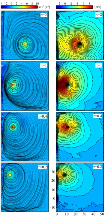
Figure 12 (left) details the vorticity map along with the 2D streamlines for the 10◦ incidence at four clearances. Each part of the figure represents an area of 50 × 50 mm surrounding the vortex. Outside the vortex core, the flow is irrotational except for the wall boundary-layer region. For
the τ = 1 case, the leakage vortex induces flow separation on the test section wall, as visible on the upper left of the figure. The wall boundary-layer with its counter-rotating vorticity is indeed entrained by the nearby TLV, as also reported by Miorini et al. (2012). As the gap is reduced, the TLV feels the neighboring wall and starts to migrate upward. The squeezing of the streamlines between the vor-tex center and the wall suggests a higher flow rate in this region. The inclination angle between the vortex axis and the measurement plane results in an apparent vortex asym-metry, as illustrated in Fig. 12 (right) with the isocontours of the circumferential velocity around the TLV axis. The contours depict a crescent-shaped region with a bump of high circumferential velocity between the wall and the TLV center, particularly visible in the τ = 1 case where the incli-nation angle is ~10°. As a consequence, the location of the maximum vorticity does not correspond exactly to the vor-tex swirl center of rotation. On the contrary, the algorithm of Graftieaux for the identification of the vortex center (c.f. Sect. 3.2) is nearly unaffected by the inclination of the TLV with respect to the measurement plane.
4.4 Axial flow evolution in TLV
Figure 13 shows the ratio of the axial flow in the vortex center to the inlet velocity as a function of τ. Values smaller than one correspond to a wake-like profile, while values greater than one correspond to a jet-like behavior. The core axial flow evolution follows the vortex intensity evolution, with an increase in the first stage of the clearance reduc-tion followed by an abrupt decline in the velocity magni-tude in highly confined situations. For instance, the 7◦ inci-dence features a small axial velocity deficit at τ = 2 which turns into a jet-like profile at τ = 0.7 before resuming a wake-like profile at τ = 0.3. As previously explained in the Sect. 4.2, the vortex core axial flow is the resulting bal-ance between an inviscid flow effect that tends to accelerate
τ=0.4 τ=1 τ=0.2 -4 -2 0 2 4 6 8 10 x103[s-1] -2 0 2 4 6 8 [m/s] τ=2 0 10 20 30 40 50 -10 0 10 20 30 τ=2 τ=1 τ=0.4 τ=0.2
Fig. 12 Left 2D streamlines of the TLV for various gap widths with the norm of the streamwise vorticity. Right isocontours of circumfer-ential velocity for various gap widths. Flow conditions: W∞= 10 m/s, incidence = 10◦, z/c = 1, rough hydrofoil
τ[-] w [-] 0.2 0.4 0.6 1 1.2 1.4 0.8 W∞ α=3° α=5° α=7° α=10° =5m/s W∞ W =10m/s∞ W =15m/s∞ W∞=20m/s 0.2 0 0.4 0.6 0.8 1 1.2 1.4 1.6 1.8 2
Fig. 13 Evolution of the vortex core axial velocity, normalized by the inlet velocity, with the normalized clearance, τ. The dashed lines are the mean values for each incidence angle
the core flow, and the momentum deficit in the boundary-layer that rolls up into the vortex core, see Eq. (7). It is thus natural that the evolution of the axial velocity follows the change of vortex intensity with confinement. Figure 14
depicts the isocontours of the axial velocity for the 10◦ incidence and illustrates the velocity evolution as the gap is reduced. The test section wall boundary-layer is clearly visible on the left-hand side at x = 0 mm. With large clear-ance values, the TLV is surrounded by the foil wake that rolls up around the vortex axis. The velocity in the vor-tex center is a jet-like profile with a peak velocity 20 % higher than the inlet velocity. The vortex strength increases slightly as the clearance is reduced to τ = 1 and the region in the TLV center with a velocity excess broadens while the foil wake is squeezed between the wall boundary-layer and the vortex center. At τ = 0.4, the vortex starts to interact with the wall boundary-layer and a region of lower than the free-stream velocity completely surrounds the TLV. The vortex still keeps a small region of high axial velocity at its center. At τ = 0.2, the vortex intensity becomes very low and the momentum defects in the boundary-layer overcome the core flow acceleration predicted by inviscid flow theory. As a consequence, a large wake-like region is present in the vortex core.
4.5 TLV position and wandering
Figure 15 (top) depicts the vortex center position with the corresponding gap width. xc represents the spanwise dis-tance between the lateral wall and the vortex center, while yc is the distance in the upward direction between the
vortex center and the hydrofoil pitching axis, cf. Fig. 1. As the clearance is reduced, the vortex naturally moves closer to the test section wall. However, a sudden increase in xc is observed around the clearance corresponding to the maximum vortex intensity—i.e., τ = 0.3, 0.4, 0.5, 0.7 for the incidence angles of 3◦, 5◦, 7◦ and 10◦—before the vor-tex center resumes its migration toward the wall. A clear physical explanation of this phenomenon is still lacking. It is assumed that the position of the vortices merging along the chord, as described in the Sect. 4.1, plays a key role in the TLV’s final strength and position.
The wall proximity also affects the vortex vertical posi-tion, as depicted in Fig. 15. At large clearances, the vortex position is independent of the operating conditions (i.e., the incidence angle and inlet velocity). As the confinement increases, the vortex migrates upward. This displacement, which is more pronounced for high incidence angles, is characteristic of a vortex–wall interaction, modeled by an image vortex. The velocity induced by the image vor-tex depends both on the vorvor-tex strength and the proximity to the wall. Since the vortex strength diminishes at small clearances, this upward migration reaches a plateau, the value of which is linked to the foil incidence angle.
The wandering amplitude in the x- and y-directions rela-tively to the gap width is depicted in Fig. 15 (bottom) with the standard deviation of the mean vortex center location. The wandering amplitude remains fairly constant for all the clearance values, except in the most confined situations
τ=2 τ=1 τ=0.4 τ=0.2 0 10 20 30 40 50 -10 0 10 20 30 [m/s] 4 6 8 10 12
Fig. 14 Isocontours of the axial velocity for different gap widths. Flow conditions: W∞= 10 m/s, incidence = 10◦, z/c = 1, rough
hydrofoil 0 0.5 1 1.5 [-] h yc 0 0.5 1 1.5 2 2.5 [-] 0 0.5 1 1.5 2 3 h xc 0 0.5 1 1.5 2 0 0.1 0 0.5 1 1.5 2 0.2 0.3 0.4 σx h[-] σhy[-] α=3° α=5° α=7° α=10° =5 m/s W∞ =15 m/s W∞ =20 m/s W∞ =10 m/s W∞ 2 τ [-] τ [-] τ [-] τ [-]
Fig. 15 Evolution of the vortex center position (top) and wandering amplitude (bottom) with the normalized clearance τ. The dashed lines are the mean values for each incidence angle. The x-direction is rep-resented on the left-hand side, while the y-direction is on the right-hand side
where it becomes very large (especially in the y-direc-tion). No significant variation of the vortex core size was observed with the confinement.
5 Conclusion
Experiments are carried out on the influence of the clear-ance size on the TLV structure in a simplified case study. A NACA0009 hydrofoil is used as a generic blade in a water tunnel while the clearance between the blade tip and the wall is varied. The 3D velocity fields are measured using SPIV for different values of the upstream velocity, the inci-dence angle and a large number of tip clearances. The wan-dering of the vortex is filtered out in the averaging process of the velocity field to obtain accurate vortex properties. A total of 1,170 distinct flow configurations are tested, yield-ing an extensive experimental database.
High-speed flow visualizations, with cavitation used as a tracer, have shown qualitatively that both the vortex tra-jectory and intensity are strongly influenced by the wall proximity. It also highlighted the clearance flow alteration, turning into a wall jet as the tip clearance is reduced. SPIV measurements confirmed that the smaller the clearance, the more the vortex is pulled away from the hydrofoil. Moreo-ver, it was observed that neither the vortex trajectory nor the wandering amplitude is altered by the TLV cavita-tion. Finally, the wake-like or jet-like nature of the axial flow profile in the vortex core is determined by the TLV intensity.
For each hydrofoil incidence angle, the systematic measurements clearly reveal the existence of a specific tip clearance for which the vortex intensity is maximum. By introducing a new dimensionless coefficient τ/Γ∗
∞, we show that the TLV circulation reaches a peak intensity for τ/Γ∗
∞≈ 0.2, which is 20–60 % higher than the unconfined case, regardless of the operating conditions. Such situations should be avoided in hydraulic axial turbomachinery, as they are the most prone to generating cavitation and lead to severe blade erosion.
Acknowledgments The present study was performed within the framework of the HydroNet project (hydronet.epfl.ch). The authors would like to thank the Competence Center of Energy and Mobility (CCEM) and swisselectric research for their financial support.
References
Arndt RE (2002) Cavitation in vortical flows. Annu Rev Fluid Mech 34(1):143–175
Ausoni P, Zobeiri A, Avellan F, Farhat M (2012) The effects of a tripped turbulent boundary layer on vortex shedding from a blunt trailing edge hydrofoil. J Fluids Eng 134(5):051207–051207. doi:10.1115/1.4006700
Batchelor GK (1964) Axial flow in trailing line vortices. J Fluid Mech 20:645–658. doi:10.1017/S0022112064001446
Bhagwat MJ, Leishman JG (2002) Generalized viscous vortex model for application to free-vortex wake and aeroacoustic calculations. In: Annual forum proceedings-American Helicopter Society. American Helicopter Society, Inc, vol 58, pp 2042–2057
Bhagwat MJ, Ramasamy M (2012) Effect of tip vortex aperiodicity on measurement uncertainty. Exp Fluids 53(5):1191–1202 Bouillot P, Brina O, Ouared R, Lovblad K, Pereira VM, Farhat M
(2014) Multi-time-lag PIV analysis of steady and pulsatile flows in a sidewall aneurysm. Exp Fluids 55(6):1–11
Boulon O, Callenaere M, Franc JP, Michel JM (1999) An experimen-tal insight into the effect of confinement on tip vortex cavitation of an elliptical hydrofoil. J Fluid Mech 390:1–23
Chang NA, Yakushiji R, Dowling DR, Ceccio SL (2007) Cavita-tion visualizaCavita-tion of vorticity bridging during the merger of co-rotating line vortices. Phys Fluids (1994-present) 19(5):058106. doi:10.1063/1.2732264
Chen G, Marble F, Greitzer E, Tan C (1991) Similarity analysis of com-pressor tip clearance flow structure. J Turbomach 113(2):260–269 Del Pino C, Parras L, Felli M, Fernandez-Feria R (2011) Structure of
trailing vortices: comparison between particle image velocimetry measurements and theoretical models. Phys Fluids 23(013):602 Devenport WJ, Rife MC, Liapis SI, Follin GJ (1996) The structure
and development of a wing-tip vortex. J Fluid Mech 312:67–106. doi:10.1017/S0022112096001929
Doligalski T, Smith C, Walker J (1994) Vortex interactions with walls. Annu Rev Fluid Mech 26(1):573–616
Fabre D, Fontane J, Brancher P, Le Dizes S, Roy C, Leweke T, Fernan-dez-Feria R, Parras L, del Pino C (2008) Synthesis on vortex mean-dering. Technical report, STREP project no. AST4-CT-2005-012238 Farrell K, Billet M (1994) A correlation of leakage vortex cavitation
in axial-flow pumps. J Fluids Eng 116(3):551–557
Gopalan S, Katz J, Liu HL (2002) Effect of gap size on tip leakage cavitation inception, associated noise and flow structure. J Fluids Eng 124(4):994–1004
Graftieaux L, Michard M, Grosjean N (2001) Combining PIV, POD and vortex identification algorithms for the study of unsteady turbulent swirling flows. Meas Sci Technol 12:1422–1429. doi:10.1088/0957-0233/12/9/307
Green SI (1995) Fluid vortices: fluid mechanics and its applications, vol 30. Springer, Berlin
Iungo G, Skinner P, Buresti G (2009) Correction of wandering smoothing effects on static measurements of a wing-tip vortex. Exp Fluids 46(3):435–452. doi:10.1007/s00348-008-0569-2 Laborde R, Mory M, Chantrel P (1997) Tip clearance and tip vortex
cavitation in an axial flow pump. J Fluids Eng 119(3):680–685 Le Guen A, Viot X, Billard JY, Fruman D (1997) Fluctuations des
vitesses et biais spatial dans le tourbillon marginal. Sixièmes Journées de l’Hydrodynamique 317–328
Lee T, Pereira J (2010) Nature of wakelike and jetlike axial tip vortex flows. J Aircr 47(6):1946–1954
McCormick B (1962) On cavitation produced by a vortex trailing from a lifting surface. J Fluids Eng 84(3):369–378
Miorini RL, Wu H, Katz J (2012) The internal structure of the tip leakage vortex within the rotor of an axial waterjet pump. J Tur-bomach 134(3):031,018
Moore DW, Saffman PG (1973) Axial flow in laminar trailing vorti-ces. Proc R Soc Lond Ser A Math Phys Sci 333(1595):491–508 Müller A, Dreyer M, Andreini N, Avellan F (2013) Draft tube
dis-charge fluctuation during self-sustained pressure surge: fluores-cent particle image velocimetry in two-phase flow. Exp Fluids 54(4):1–11. doi:10.1007/s00348-013-1514-6
Pasche S, Gallaire F, Dreyer M, Farhat M (2014) Obstacle-induced spiral vortex breakdown. Exp Fluids 55(8):1–11. doi:10.1007/ s00348-014-1784-7
Prasad AK (2000) Stereoscopic particle image velocimetry. Exp Flu-ids 29(2):103–116. doi:10.1007/s003480000143
Roussopoulos K, Monkewitz PA (2000) Measurements of tip vortex characteristics and the effect of an anti-cavitation lip on a model Kaplan turbine blade. Flow Turbul Combust 64(2):119–144 Spalart PR (1998) Airplane trailing vortices. Annu Rev Fluid Mech
30(1):107–138
Vatistas GH, Kozel V, Mih W (1991) A simpler model for concen-trated vortices. Exp Fluids 11(1):73–76
van der Wall BG, Richard H (2006) Analysis methodology for 3C-PIV data of rotary wing vortices. Exp Fluids 40:798–812. doi:10.1007/s00348-006-0117-x
Wang Y, Devenport WJ (2004) Wake of a compressor cascade with tip gap, part 2: effects of endwall motion. AIAA J 42(11):2332–2340 Westerweel J (2000) Theoretical analysis of the measurement preci-sion in particle image velocimetry. Exp Fluids 29(1):S003–S012. doi:10.1007/s003480070002
Wu H, Tan D, Miorini RL, Katz J (2011) Three-dimensional flow structures and associated turbulence in the tip region of a water-jet pump rotor blade. Exp Fluids 51(6):1721–1737. doi:10.1007/ s00348-011-1189-9