MIT Joint Program on the
Science and Policy of Global Change
Carbon Emissions and The Kyoto Commitment
in the European Union
Laurent L. Viguier, Mustafa H. Babiker and John M. Reilly
Report No. 70
The MIT Joint Program on the Science and Policy of Global Change is an organization for research, independent policy analysis, and public education in global environmental change. It seeks to provide leadership in understanding scientific, economic, and ecological aspects of this difficult issue, and combining them into policy assessments that serve the needs of ongoing national and international discussions. To this end, the Program brings together an interdisciplinary group from two established research centers at MIT: the Center for Global Change Science (CGCS) and the Center for Energy and Environmental Policy Research (CEEPR). These two centers bridge many key areas of the needed intellectual work, and additional essential areas are covered by other MIT departments, by collaboration with the Ecosystems Center of the Marine Biology Laboratory (MBL) at Woods Hole, and by short- and long-term visitors to the Program. The Program involves sponsorship and active participation by industry, government, and non-profit organizations.
To inform processes of policy development and implementation, climate change research needs to focus on improving the prediction of those variables that are most relevant to economic, social, and environmental effects. In turn, the greenhouse gas and atmospheric aerosol assumptions underlying climate analysis need to be related to the economic, technological, and political forces that drive emissions, and to the results of international agreements and mitigation. Further, assessments of possible societal and ecosystem impacts, and analysis of mitigation strategies, need to be based on realistic evaluation of the uncertainties of climate science.
This report is one of a series intended to communicate research results and improve public understanding of climate issues, thereby contributing to informed debate about the climate issue, the uncertainties, and the economic and social implications of policy alternatives. Titles in the Report Series to date are listed on the inside back cover.
Henry D. Jacoby and Ronald G. Prinn,
Program Co-Directors
For more information, please contact the Joint Program Office
Postal Address: Joint Program on the Science and Policy of Global Change 77 Massachusetts Avenue
MIT E40-271
Cambridge MA 02139-4307 (USA) Location: One Amherst Street, Cambridge
Building E40, Room 271
Massachusetts Institute of Technology Access: Phone: (617) 253-7492
Fax: (617) 253-9845
E-mail: g l o b a l c h a n g e @ m i t . e d u
Web site: h t t p : / / M I T . E D U / g l o b a l c h a n g e /
Carbon Emissions and The Kyoto Commitment
in the European Union
Laurent L. Viguier*†, Mustafa H. Babiker*, and John M. Reilly*
Abstract
We estimate reference CO2 emission projections in the European Union, and quantify the economic impacts of the Kyoto commitment on Member States. We consider the case where each EU member individually meets a CO2 emissions target, applying a country-wide cap and trade system to meet the target but without trade among countries. We use a version of the MIT Emissions Prediction and Policy Analysis (EPPA) model, here disaggregated to separately include 9 European Community countries and commercial and household transportation sectors. We compare our results with that of four energy-economic models that have provided detailed analyses of European climate change policy. In the absence of specific additional climate policy measures, the EPPA reference projections of carbon emissions increase by 14% from 1990 levels. The EU-wide target under the Kyoto Protocol to the Framework Convention on Climate Change is a reduction in emissions to 8% below 1990 levels. EPPA emissions projections are similar to other recent modeling results but there are underlying differences in energy and carbon intensities among the projections. If EU countries were to individually meet the EU allocation of the Community-wide carbon cap specified in the Kyoto Protocol, we find using EPPA that carbon prices vary from $91 in the United Kingdom to $385 in Denmark; welfare costs range from 0.6 to 5%.
Keyword(s): Global change; CO2 emissions; Abatement costs; Kyoto Protocol; European Union; Computable general equilibrium model.
Contents
1. INTRODUCTION... 2
2. THE EPPA-EU MODEL... 3
2.1. EU Disaggregation... 3
2.2. Transportation Sector Disaggregation ... 5
3. OTHER ECONOMIC MODELS ... 6
4. THE REFERENCE CASE FOR EUROPE ... 8
4.1. Assumptions and Reference Projections of EPPA-EU ... 8
4.2. Reference Projections for CO2 Emissions in EPPA-EU ... 10
4.3. Comparison of CO2 Projections... 12
4.4. Decomposition of Emissions Intensities of GDP... 15
5. EMISSIONS ABATEMENT COST AND CLIMATE POLICIES... 20
5.1. Reference Emissions Projections and Burden sharing Agreement ... 20
5.2. Emissions Abatement Costs in Europe ... 22
5.3. Welfare Costs and Competitiveness Effects ... 27
6. CONCLUSION ... 28
7. ACKNOWLEDGEMENTS ... 29
8. REFERENCES... 30
* Joint Program on the Science and Policy of Global Change, Massachusetts Institute of Technology, MA. † Institute of Energy Policy and Economics, CNRS, Grenoble.
1. INTRODUCTION
At the Third Conference of the Parties (COP-3) to the United Nations Framework Convention on Climate Change (UNFCCC), Annex B1 Parties committed to reducing, either individually or jointly, their total emissions of six greenhouse gases (GHGs) by at least 5 percent within the period 2008 to 2012, relative to these gases’ 1990 levels.
The European Union (EU) is a full Party to the UNFCCC and a signatory of the Kyoto Protocol, and has accepted a quantitative absolute reduction of 8 percent of its GHG emissions. Article 4 of the Protocol allows the EU to allocate its target among the Member States. A political agreement on that redistribution was reached at the environmental Council meeting on June 1998, and is referred to as the “Burden Sharing” Agreement (BSA).
The Kyoto Protocol allows Annex B Parties to meet their commitments by three “flexible mechanisms” (emission trading, clean development mechanism, and Joint Implementation) in order to reduce the economic cost of emissions reductions. Flexible mechanisms could be implemented at the European level: in March 2000, the European Commission prepared a “Green Paper on greenhouse gas emissions trading within the European Union” that proposes to introduce in 2005 an EU trading system that would be integrated into the international trading system in 2008 (Viguier, 2000). They could also be implemented at national level: e.g., emissions trading systems are in the process of being established in Norway, the United Kingdom, and Denmark; and other countries, namely, Sweden, France, and most recently
Germany, have advanced proposals or announced intentions to include emissions trading systems as part of their plans for implementation of the Kyoto Protocol (Ellerman, 2000).
The primary objective of this paper is to develop a version of the MIT Emissions Prediction and Policy Analysis (EPPA) model and a reference emissions projection to study the economic impacts of restricting CO2 emissions in the European Union. As reference emissions growth is an
important factor in estimating the costs of meeting an emissions target, we make a detailed comparison of trends in energy intensities, economic growth, emissions profiles, and abatement costs curves in EPPA with those resulting from other models that are popular in the climate change policy discussions in Europe. The other models we consider in this paper are POLES-IEPE, PRIMES-NTUA, WEPS-EIA, and GTEM-ABARE. Such a comparison is important for understanding the differences in the economic impacts of Kyoto on Annex B regions produced by these models. In section 2, we provide a brief description of the new version of the EPPA model developed for this analysis (EPPA-EU) including 9 EU countries and the addition of a transportation sector in households and in industry for each of these countries. We also briefly describe the other models chosen for the comparison. In section 3, we present the emission reference projected for European countries in the EPPA model, and compare it with reference cases in the other models. In section 4, we consider the economic impact for European countries of implementing the Kyoto target, and the Burden Sharing Agreement, without flexibility mechanisms. Marginal abatement cost curves and domestic carbon price estimates are compared
in this section with the other economic models. Finally, section 5 draws conclusions from our findings.
2. THE EPPA-EU MODEL
The Emissions Prediction and Policy Analysis (EPPA) model is a recursive dynamic multi-regional general equilibrium model of the world economy that has been developed for analysis of climate change policy (Babiker et al., 2000a, Babiker et al., 2000b, Babiker et al., 2000c,
Ellerman and Wing, 2000, Babiker and Eckaus, 2000, and Babiker and Jacoby, 1999). Previous versions of the model have been used extensively for this purpose (e.g., Jacoby et al., 1997; Ellerman and Decaux, 1998; Jacoby and Sue Wing, 1999; and Reilly et al., 1999).
The current version of EPPA is built on a comprehensive energy-economy data set (GTAP4-E2) that accommodates a consistent representation of energy markets in physical units as well as detailed accounts of regional production and bilateral trade flows. The base year for the model is 1995 and it is solved recursively at 5-year intervals. A full documentation of the current version of EPPA is provided in Babiker et al., 2000d.
2.1. EU Disaggregation
EPPA-EU extended the current version of EPPA by bringing in a detailed breakdown of the EU and incorporating an industry and a household transport sectors for each region. The
regional, sectoral, and factors aggregation shown in Table 1, together with the substitution elasticities in Table 2 completely specify the benchmark equilibrium.
The European Union is disaggregated into 9 countries and 1 region representing the Rest of Europe (ROE). Four out of the 9 EU countries (France, Spain, Italy, and the Netherlands) were aggregated together with ROE in the GTAP4-E database.
We disaggregated this region using data from the GTAP-5 Pre-release that provides a complete disaggregation of the EU.3 To accomplish this task we developed an optimization algorithm that uses the economic structure of these 4 countries in GTAP-5 Pre-release while imposing the output, demand, and trade balances for their corresponding aggregate region in GTAP4-E. This allowed us to leave unchanged all other regions of the standard EPPA based on GTAP4-E.
2 For description of the GTAP database see Hertel, 1997.
3 Though GTAP-5 Pre-release has all 9 of these countries broken out we chose to focus on disaggregating only the 4 largest of these countries.
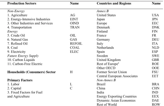
Table 1. Dimensions of the EPPA-EU model
Production Sectors Name Countries and Regions Name
Non-Energy Annex B
1. Agriculture AG United States USA
2. Energy-Intensive Industries EINT Japan JPN
3. Other Industries and Services OIND Europe EEC
4. Transportation TRAN Denmark DNK
Energy Finland FIN
5. Crude Oil OIL France FR
6. Natural Gas GAS Germany DEU
7. Refined Oil REFOIL Italy ITA
8. Coal COAL Netherlands NLD
9. Electricity ELEC Spain ESP
Future Energy Supply Sweden SWE
10. Carbon Liquids United Kingdom GBR
11. Carbon-Free Electric Rest of Europea ROE
Other OECD OOE
Households (Consumers) Sector H Former Soviet Union FSU
Central European Associates EET
Primary Factors Non-Annex B
1. Labor L Brazil BRA
2. Capital C China CHN
3. Fixed Factors for Fuel India IND
and Agriculture Energy Exporting Countries EEX
Dynamic Asian Economies DAE
Rest of World ROW
Notes: a Includes Austria, Belgium, Greece, Ireland, Luxemburg, and Portugal.
Table 2. EPPA-EU Model Default Parameters
Parameter Description Value Comments
σERVA Elasticity of substitution between energy
resource composite and value-added 0.6 Agriculture only
σER Substitution between land and
energy-material bundle
0.6 Agriculture
σAE Substitution between energy and material
composite 0.3 Agriculture
σVA Substitution between labor & capital 1 All sectors except nuclear in which is 0.5
σENOE Substitution between electric and non
electric energy
0.5 All sectors
σEN Substitution among non-electric energy 1 All sectors except for electricity where coal and oil generation substitute
at 0.3 among themselves and at 1 with gas
σGR Substitution between fixed factor and the
rest of inputs
0.6 All sectors that have fixed resource, except nuclear generation where it is
calibrated to match exogenous supply elasticity
σEVA Substitution between energy and value
added composite
0.4 For all sectors except energy intensive and other industry where it is 0.5
σDM Armington substitution between domestic
and imports 3 All goods except Electricity where it is 0.3
σMM Armington substitution across imports 5.0
4.0
Non-energy goods
Energy goods, except refined oil (6) and electricity (0.5)
σCS Temporal substitution between
consumption and saving 1 Final demand sector
σC Substitution across consumption goods Varies across countries and is updated with income recursively to reflect
income elasticities based on an econometrically estimated equation
G0 Labor supply annual growth rate in
efficiency units
2% 2.5-6%
For developed countries and converges to 1 by 2100 For developing countries and converges to 1.5% by 2100
2.2. Transportation Sector Disaggregation
The other change in this version of the model is the disaggregation of the transportation sector. With transportation disaggregated, there are now nine output sectors for each of the 22 regions in EPPA-EU, as shown in the left-hand column of table 1. The EPPA model also includes future or “backstop” sources of fuels and electricity, but they do not play a significant role in this analysis which looks only out to 2020. Eight of the production sectors follow the standard EPPA definitions. The ninth, transportation (denoted TRAN), has been added by this study. The GTAP database does not include a separate transportation sector within industry, nor does it contain a separate category for private automobile services in the household sector. We followed the methodology developed by Babiker et al., 2000c for the United States to break out transportation from EPPA’s OTHERIND sector and to create a household supplied
transportation sector (i.e. private automobiles) in the EU.
The basic approach for the TRANS sectors is to use GTAP’s trade and transport sector that combines transport with trade margins in combination with data from Input-Output tables produced by the European statistical office (Eurostat). These tables provide the data to
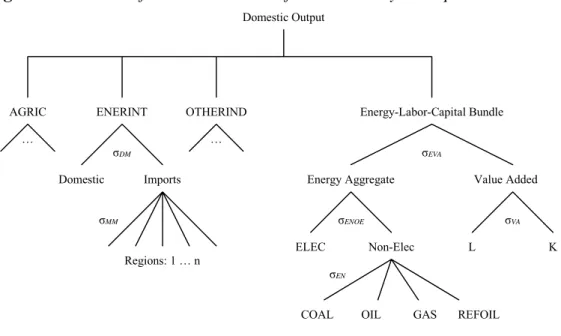
disaggregate trade margins from transportation for each European country. For the other regions in the model, we used the US input-output coefficients from Babiker et al., 2000c study. The TRANS industry supplies transportation services (both passenger and freight) to other sectors and to households. The structure of the transportation industry sector is depicted in Figure 1.
Figure 1. Structure of Production Sector for the Industry Transportation Sector
Domestic Output
AGRIC ENERINT OTHERIND Energy-Labor-Capital Bundle
Domestic Imports Energy Aggregate Value Added
ELEC Non-Elec L K Regions: 1 … n
COAL OIL GAS REFOIL
σDM σEVA σVA σENOE σEN σMM … …
We have also made adjustments directly to the Household (H) sector to represent own-supplied transportation services, primarily that provided by personal automobiles. Households produce transportation services for their own consumption using inputs from the Other Industry
Products (OIND) and Refined Oil sectors. Consumption expenditure of private households reported by Eurostat (1999) and energy statistics from the International Energy Agency (IEA, 1998a; IEA, 1998b; IEA, 2000) along with the coefficients reported in the Babiker et al., 2000c study were used to separate the household purchases that are part of household production of transportation from other household purchases.
The new breakout yields a sector of own-supplied personal transportation (private automobiles) separate from other household activities, and a separate transportation sector in industry that supplies transport services to both industry (i.e., freight transportation and any passenger transportation purchased by business) and households (purchased transportation service, mainly passenger transportation services such as air and rail service). Services from private automobiles involve inputs from OIND that include the automobile itself, repairs, insurance, parking, and vehicle fuel from the REFOIL sector. The procedure involves allocating OIND and REFOIL output between direct uses in the household. The structure of personal transportation services within the household sector is illustrated in Figure 2.
Figure 2. Structure of Household Sector with Transportation
Consumer Utility Aggregate Consumption Savings Consumption IND, 1-6* OTHER IND, H REFOIL, H TRANSPORT, H PRIVATE AUTOS TRANSPORT OTHER IND, PA REFOIL, PA σCS σ = 1 σC σDM σ = 0 σ = 0.5
* AG, EINT, OIL, GAS, COAL, ELEC
Regions: 1 … n
σMM
Domestic Imports
3. OTHER ECONOMIC MODELS
We compare the EPPA-MIT reference for Europe with reference projections of 4 other models: POLES-IEPE, PRIMES-NTUA, WEPS-EIA, and GTEM-ABARE.
The POLES model, developed at IEPE (Institut d’Economie et de Politique de l’Energie-CNRS), is a global partial equilibrium model of the world energy system with 30 regions. POLES can produce detailed world energy and CO emission projections by region through the
year 2030. POLES combines some features of “top-down” models in that prices play a key role in the adjustment of most variables in the model but retains detail in the treatment of
technologies characteristic of “bottom-up” models. The dynamics of the model is given by a recursive simulation process that simulates energy demand, supply and prices adjustments (Criqui et al. 1996). Marginal abatement cost curves for CO2 emissions reductions are assessed
by the introduction of a carbon tax in all areas of fossil fuel energy use. This carbon tax leads to adjustments in the final energy demand within the model, through technological changes or implicit behavioral changes, and through replacements in energy conversion systems for which the technologies are explicitly defined in the model. The POLES’ model has been already used to analyze economic impacts of climate change policies and the consequences of implementing flexibility mechanisms (e.g., Blanchard et al., 2000; Criqui et al., 1999; Criqui and Viguier, 2000a; Criqui and Viguier, 2000b, Criqui et al., 2000).
The PRIMES (version 2) model is a partial equilibrium model of the European energy system and market developed by the Institute of Communication and Computer Systems of National Technical University of Athens (Capros and Mantzos, 1999). The model simulates the overall market equilibrium of the energy sector according to the mixed-complementary
methodology, which roughly correspond to the Kuhn-Tucker conditions of a mathematical programming problem. The current version of the model (version 2) formulated as a non-linear mixed complementarity (MCP) problem and solved under GAMS/CPLEX/PATH is calibrated on 1995 data set for all European Union Member States. It computes the prices of energy products that lead to the balancing of demand and supply of each energy product in a period of time (five year period). The model computes a static equilibrium each period, driven by
exogenous assumptions about economic and population growth between periods. The imposition of carbon emissions constraint gives rise to a shadow price of carbon. The mechanism through which the energy system responds to the imposition of carbon constraints is that of changes in relative energy prices. These changes reflect the carbon content of each fuel and provide
incentives to the economic agents to reduce their “consumption” of carbon. This model has been used to analyze macro-economic and sectoral effects of alternative climate policies for Europe (e.g., Capros et al., 2000; Capros and Mantzos, 2000).
The World Energy Projection System (WEPS) is a partial equilibrium model of the world energy system developed by the US Energy Information Administration to provide a consistent, integrated, economic, and flexible accounting framework for analyzing and projecting trends in world energy markets (EIA, 1997). WEPS provides historical data and 2020 projections of energy consumption across the range of primary energy sources for major countries and regions worldwide (EIA, 2000). The WEPS accounting framework incorporates projections from independently documented models and assumptions about the future energy intensity of economic activity (ratios of total energy consumption divided by gross domestic product), and about the rate of incremental energy requirements met by natural gas, coal, and renewable energy sources (hydroelectricity, geothermal, solar, wind, biomass, and other renewable resources). Two independently documented models, the International Energy Module (IEM)—a module of the National Energy Modeling System (NEMS)—and the International Nuclear Model, PC Version (PC-INM) provide projections of oil and nuclear power consumption, respectively, which are incorporated into the WEPS model.
The GTEM model is a recursive dynamic general equilibrium model of the world economy developed by the Australian Bureau of Agricultural and Resources Economics (ABARE, 1996). Built on the GTAP database version 4.0e, GTEM includes 50 industries in 45 countries and regions. The regional coverage includes detail only for 5 EU countries: Denmark, Finland, Germany, Sweden, and the United Kingdom. Unlike the other models consider in this study, the greenhouse gas coverage in GTEM is not limited to carbon dioxide – it include methane and nitrous oxide – and include removals by forest sinks. The GTEM model has been used to analyze the economic impacts of the Kyoto Protocol on different regions, such as developing countries and European countries (Brown et al., 1999; Polidano et al., 2000; Jotzo et al., 2000).
4. THE REFERENCE CASE FOR EUROPE
4.1. Assumptions and Reference Projections of EPPA-EU
Costs estimates of climate change policies depend crucially on reference assumptions for economic growth, energy prices, the evolution of the electricity sector, and the resulting CO2
emissions without any change in energy and environmental regulations.
Technological growth in EPPA-EU is labor-augmented. The productivity parameter in EPPA-EU is adjusted such that the GDP growth rates during 1995-2000 approximate those estimated by IMF (2000). Table 2 displays our reference economic growth projections and IMF estimates of growth for 1995-2000. Real GDP growth rates are projected to be in the range of 2.5%-2.9% through 2020 in Europe. These growth rates are lower than in the United States, but higher than in Japan. Economic growth is projected to be higher in Southern Europe (Spain, Portugal, and Greece) than in Northern Europe, except for Finland, Netherlands, and Sweden.
Table 2. Real GDP Growth Rates, Reference scenario (%) IMF 1995 -2000 1995 -2010 2010 -2020 DEU 1.7 2.4 2.5 DNK 2.4 3.0 3.1 ESP 3.6 3.8 4.0 FIN 4.9 4.1 4.3 FR 2.5 2.6 2.6 GBR 2.8 2.8 2.8 ITA 1.8 2.2 2.3 NLD 3.6 3.5 3.4 SWE 2.8 3.2 3.5 ROE 3.5 3.6 3.5 EEC 2.6 2.8 2.9 USA 4.3 3.4 3.4 JPN 1.1 1.9 2.3
Sources: IMF (2000), and EPPA-EU.
Table 3 shows the main assumptions for energy prices in the European Union. Energy
prices are projected to rise gradually over the period. In EPPA, energy prices through 2010 are exogenously set in the reference case and then allowed to vary from this reference in response to climate policy. After 2010, prices in the reference and policy cases are endogenously determined by a long run resource model. Given the 5-year time step of the EPPA model, there is no attempt to represent processes that give rise to large short-run variability in energy prices. Coal prices increase at higher rates in Europe than in the United States or in Japan. On average, the increase of coal prices is projected to be lower than the increase of natural gas and oil prices between 1995 and 2020 (except in Germany where the demand for coal remains very high). The increase of oil prices is higher than coal and natural gas prices during the whole period.
Table 3. Reference Projections on Energy Prices
(Average % Change Per Year) 1995 -2010 2010 -2020 1995 -2010 2010 -2020 1995 -2010 2010 -2020 DEU 3.2 2.4 2.4 2.0 3.7 3.0 DNK 1.3 1.0 2.7 3.0 3.7 3.0 ESP 3.0 2.3 2.8 2.8 3.7 3.0 FIN 2.1 1.5 3.0 2.3 3.7 3.0 FR 2.0 1.3 2.8 2.5 3.7 3.0 GBR 2.9 2.1 2.7 3.0 3.7 3.0 ITA 3.0 2.1 2.9 2.7 3.7 3.0 NLD 1.6 1.2 2.7 3.0 3.7 3.0 SWE 1.6 1.2 2.8 2.3 3.7 3.0 ROE 2.3 1.6 3.2 2.7 3.7 3.0 USA 1.5 1.0 2.7 2.0 3.7 3.0 JPN 1.1 0.8 2.7 2.0 3.7 3.0
Coal Gas Oil
The share of various technologies in electricity generation is projected to remain largely unchanged from the 1995 base year through to 2020. For the EU as a whole, coal accounts for about 60 percent of fossil use used in electricity generation with gas and oil each accounting for approximately 20 percent. Among countries these shares vary but for each country shares through 2020 are not projected to change substantially in the reference. For example, coal accounts for nearly 80 percent of fossil fuel used in electricity in Germany and Denmark and between 65 and 70 percent in Spain and Great Britain and these shares are not projected to change substantially. Among EU countries, Italy was least dependent on coal (less than 10 percent) in 1995 and most dependent on oil for electricity (greater than 60 percent), with little change in these shares through 2020. Gas as a share of fossil fuels used in the electric sector ranged from under 10 percent in Spain to over 25 percent in Great Britain and Italy in 1995, again with little change in these shares projected through 2020. Most other countries are not far from the EU average. Capital asset fixity and small changes in the relative prices of oil, gas, and, coal combine to give this result.
Nuclear power generation is a separate sector in EPPA that includes a fixed factor input that can be used to limit expansion or force a contraction of the sector to reflect policy decisions
(Babiker, Reilly, Ellerman, 2000). The fixed factor growth was set to approximate the change in nuclear power production as in the EC projections shown in Table 4 (EC, 1999). The EC
projections assume that it will be possible to extend the technical lifetime of old nuclear plants up to 40 years. It also assumed that EU countries without installed nuclear capacity in 1995 would not invest in nuclear energy over the outlook period. This reference EC projection also takes into account the decommissioning schedules for nuclear power that have been recently decided at national level for Germany, Sweden, Netherlands, and Spain. The EC projections assumed that the agreement signed in Germany to retire 19 nuclear reactors by 2021 is progressively implemented from 2005. This set of projections differs from those of GTEM (Jotzo, 2000) that assumes that the share of nuclear power in electric generation is projected to be unchanged before 2020.
Table 4. Forecasts for Nuclear Production,
Reference Scenario (Average % Change Per Year) 1995 -2000 2000 -2005 2005 -2010 2010 -2015 2015 -2020 DEU 1.94 0.00 -0.23 -3.10 -6.62 DNK - - - - -ESP 0.83 0.00 0.00 -0.41 -1.26 FIN 1.17 1.82 0.00 0.00 -0.35 FR 1.73 0.79 0.21 0.79 0.20 GBR 2.41 0.69 -0.61 -4.57 -1.93 ITA - - - - -NLD 1.92 -3.93 -100 - -SWE 0.22 -0.22 0.00 -3.45 -7.01 ROE 2.58 0.34 -0.34 0.00 -1.23
Source: European Commission, 1999
4.2. Reference Projections for CO2 Emissions in EPPA-EU
In the EPPA-EU model, CO2 emissions in EU countries are projected to reach 3.8 GtCO2 in 2010
and 4.1 GtCO2 in 2020 in the reference case. On average, projected growth rates of emissions for
Europe are lower than in the United States, but higher than in Japan (Table 5). Emissions are projected to increase by 1.07 per year between 1995 and 2010, slowing to 0.64 per year between 2010 and 2020.Table 5 also shows significant differences among EU countries. Future emissions growth is slowest in the United Kingdom and Germany. Emissions growth rates in France are projected to be very closed to average growth rates in the European Union for the whole period. In contrast, reference emissions growth is projected to be very high in Spain, Finland and Sweden
Table 5. Projected CO2 Emissions Growth by Country, Reference Scenario (Average % Change Per Year)
1995 -2010 2010 -2020 DEU 0.59 0.03 DNK 1.36 0.81 ESP 2.56 1.62 FIN 2.35 1.74 FR 1.17 0.67 GBR 0.54 0.11 ITA 0.45 0.61 NLD 1.65 0.58 SWE 2.44 1.40 ROE 1.58 1.34 EEC 1.07 0.64 USA 1.58 1.02 JPN 0.96 0.90
The EPPA projections show relatively rapid growth in transportation and household emissions and slow growth in electric sector and industry emissions (Figure 1). As a result, households and transportation are projected to account for more than one-half of emissions in 2020 in the EPPA reference case, up from 37 percent in 1995. The electric sector was the largest emitter in 1995 with 28 percent of total emissions and the transportation sector was the second largest accounting for 19 percent. The transportation sector remains the second largest emitting sector of the European economy in 2020 with 24 percent of total emissions. However, the
household sector is the largest emitting sector in 2020 with 27 percent. The electricity sector falls to the third largest emitting sector. These trends are observed in all EU countries (except in Sweden where the share of transportation in national emissions decreases) although the specific sector shares in each country differ.
Figure 1. CO2 Emissions by Sector in Europe, Reference Scenario (% of Total Emissions)
0 5 10 15 20 25 30 35 40 1995 2010 2020 1995 2010 2020 1995 2010 2020 1995 2010 2020 1995 2010 2020 1995 2010 2020
Agriculture Electricity Transports Energy intensive
Other industries
Households
4.3. Comparison of CO2 Projections
Figures 2-7 show CO2 emissions trends from 1960 to 1995, and emissions projected by
economic models to 2020. Estimations for CO2 emissions are based on OECD energy balances
published by the International Energy Agency, and using the methodology of the International Panel on Climate Change (IPCC). To be able to compare emissions projections from different economic models, we apply projected emissions growth rates from our estimate of 1995 emissions levels.
The historical data show rapid growth of CO2 emissions in Japan compared to the United
States and the European Union. Japan’s emissions quadrupled from 1960 to 1995 whereas the increase was 88 percent in the US and 56 percent in the EU. Historical trends also show the higher impact of the two oil shocks on the EU compared to Japan and the US.
Emissions projections for the United States and Japan to 2010 and 2020 are similar in EPPA-EU, GTEM and the WEPS model of the DOE. POLES projects lower emissions growth rates compared to these models for the United States. For Europe, emissions growth rates are projected to be higher in EPPA-EU than in other models during the whole period. EPPA-EU combines both relatively high GDP growth and rapid reductions in energy use per dollar of GDP compared with the other models. Higher emissions in EPPA are thus due primarily to higher GDP growth rates for this region (the average GDP growth rate for Europe in EPPA-EU is 3.6 percent between 1995 and 2010, 2.5 percent in POLES and PRIMES, and 2.7 percent in GTEM and WEPS).
Figures 2-7 show greater differences among the models for individual EU countries than for
the EU as a whole. There are substantial differences for Germany with little increase for GTEM and PRIMES while in POLES emissions are expected to decrease between 1995 and 2000, and to increase rapidly after this date. In EPPA-EU, emissions in Germany increase more rapidly in
early years and stabilize after 2005. These differences mean that emissions are 100 MtCO2 lower
in POLES and PRIMES than in WEPS and EPPA-EU in 2010. Emission projections are
comparable for 2010 in the United Kingdom, except in the WEPS model where the projection is surprisingly high. For France, emissions projections are similar in the different models
considered in this study, especially for 2010
Figures 2-7. CO2 Emissions, 1960-2020 (in MtCO2) United States 0 1000 2000 3000 4000 5000 6000 7000 8000 1960 1965 1970 1975 1980 1985 1990 1995 2000 2005 2010 2015 2020 MtC O 2 Observed EPPA WEPS GTEM POLES 1995 Japan 0 200 400 600 800 1000 1200 1400 1600 1960 1965 1970 1975 1980 1985 1990 1995 2000 2005 2010 2015 2020 MtC O 2 Observed EPPA WEPS GTEM POLES 1995
European Union 0 500 1000 1500 2000 2500 3000 3500 4000 4500 1960 1965 1970 1975 1980 1985 1990 1995 2000 2005 2010 2015 2020 Mr CO 2 Observed EPPA GTEM POLES PRIMES 1995 France 0 100 200 300 400 500 600 700 1960 1965 1970 1975 1980 1985 1990 1995 2000 2005 2010 2015 2020 MtC O 2 Observed EPPA WEPS POLES PRIMES 1995 Germany 0 200 400 600 800 1000 1200 1960 1965 1970 1975 1980 1985 1990 1995 2000 2005 2010 2015 2020 Mt C O 2 Observed EPPA WEPS GTEM POLES PRIMES 1995
United Kingdom 0 100 200 300 400 500 600 700 800 900 1960 1965 1970 1975 1980 1985 1990 1995 2000 2005 2010 2015 2020 Mt C O 2 Obs erved EPPA WEPS GTEM POLES PRIMES 1995
4.4. Decomposition of Emissions Intensities of GDP
Comparable emission projections across economic models can result from different and offsetting assumptions. As noted above, EPPA-EU projects only slightly higher emissions despite GDP growth rates a percentage point higher than other models. To understand this result, a useful comparison is the carbon intensity of GDP, measuring the quantity of carbon emissions associated with one dollar of GDP. It can be decomposed in two effects: 1) the change in emissions intensity of energy consumption and 2) the evolution of energy intensity of GDP. These summary measures of an economy’s carbon emissions intensity can be constructed from readily available historical data or model output. Such a decomposition of emissions intensity of GDP provides a good basis to understand the relationship between emissions and economic growth in different economies, and to make inter-model comparisons. Carbon intensity of energy changes with the evolution of the fuel mix (e.g. coal to gas substitution), and with the structure of energy consumption in the economy. The origin of temporal and spatial disparities of energy intensity of GDP can vary due to the evolution of the economic system, the structure and the efficiency of the energy system, the GDP structure, technology and varied socio-economic behaviors.
To make this comparison, we use a graphic approach already used in Viguier (1999). We convert GDP for all countries into 1990 US dollars using the 1990 exchange rates.4 Projections from all the models are normalized to actual 1995 data to preserve the forecasted trends. In
Figures 8-12, the x-axis is the energy intensity of GDP and the y-axis is the emission intensity of
energy. Light curves are isoquants for a given (constant) carbon intensity of GDP. Each point on one of these curves gives a combination of emission intensity of energy and energy intensity of GDP that results in the same level of emission intensity of GDP; i.e. an economy can achieve a
4Comparisons across countries in the absolute levels of emissions intensity and energy intensity per unit of GDP
depend on the conversion of GDP from home currency to a common currency. Exchange rate variations can be fairly large (e.g. the recent decline of the EURO) and thus the base year exchange rate chosen can have a significant effect. The time path is not affected by exchange rate variation.
given level of emissions per dollar of GDP with a high level of energy efficiency using a
relatively carbon intensive mix of fuels or with a lower level of energy efficiency combined with mix of fuels with a relatively low carbon intensity. These graphs include a decomposition of emission intensities observed between 1960 and 1995, and a decomposition of emission intensities projected in the different economic models until 2020.
We show in Figures 8-12 the isoquants of carbon intensity of GDP corresponding to the Kyoto commitment if we assume GDP growth in the EPPA-EU reference (see Table 2). These curves apply only to 2010 and to the other models only if GDP growth was that found in EPPA and that rate of growth of GDP applied to these models did not affect emissions intensity. In reality, if higher GDP growth were actually imposed in these models, one would expect higher energy prices and as a result somewhat greater energy-efficiency and a shift in fuel mix. Further economic growth beyond 2010 would require further reduction in energy intensity in all of the projections if the Kyoto target emissions levels were to be maintained.
Figure 8 shows that the reduction of the carbon intensity of US GDP has been mostly due to
the reduction of energy intensity. The data, based on 1990 exchange rates, show the carbon intensity of GDP for the US economy to have been around fifty percent higher than in Europe at the beginning of the sixties, and the gap has increased from 1960 to 1995. Most of the gain in emissions intensity of GDP in the US has been due to energy efficiency gains with little change in the carbon intensity of fuels. This tendency is projected to continue in the EPPA-EU model until 2020. In POLES and WEPS, the reduction of energy intensity is projected to be more limited, and the carbon intensity of energy consumption is projected to increase in the future, the consequence of rising coal consumption. In Europe, both the decline of energy intensity and the positive evolution of the fuel mix are responsible for a falling emissions intensity of GDP for the 1960 to 1995 period. EPPA-EU projects a slight reduction of carbon intensity of GDP in Europe due mainly to the decrease of energy intensity. Projections are similar across economic models for 2010, although PRIMES and POLES project a larger reduction of carbon intensity of energy. Based on EPPA-EU growth rate assumptions, the European Union is closer to the level of carbon intensity that would meet the Kyoto target in 2010 than is the United States.
In Japan, the historical trend in carbon intensity of GDP has three distinct periods (Figure
9). From 1960 to 1974, carbon intensity of GDP rises because the increase of energy intensity
outweighs the decline of carbon intensity of energy consumption. From 1974 to 1989, both emissions intensity of energy and energy intensity of the economy contribute to a decline in the carbon intensity of GDP. After 1989, the emission intensity of GDP of the Japanese economy rose. From 1990 to 1992 the increase is due to a fuel mix effect and from 1991 to 1995 a growth of energy intensity also contributes to the rise in emissions intensity of GDP. The EPPA-EU model projects a larger reduction of carbon intensity than the other models between 1995 and 2020 due to a higher decrease of energy intensity in this country. As in the United States, the reduction of carbon intensity in 2010 in the reference case plotted here only one-half that needed to meet the Kyoto commitment.
We also plot separately the three largest EU economies, showing that the pattern over time is not uniform across the EU. France’s aggressive nuclear program explains most of its decline of carbon intensity of GDP observed in the past (Figure 10). An important part of this trend is the
and used widely. As a result, the level of carbon intensity reached in 1995 is one of the lowest among developed economies but France shows little improvement in energy efficiency. Nuclear power is not expected to increase substantially in the future under any of the model forecasts. All show a pattern of energy efficiency improvements rather than fuel mix changes that is similar to the evolution projected for other economies. Emissions projections for France through 2010 are comparable in EPPA-EU, WEPS, and PRIMES.
In Germany, carbon intensity of GDP has decreased substantially between 1960 and 1995 due to the combined effect of the fuel mix and energy efficiency (Figure 11). The trend is expected to continue in this country in the different economic models. The decline of carbon intensity of fuels is more important in the sectoral models (POLES and PRIMES) than in EPPA-EU and WEPS. Contrary to most of other Annex B countries, Germany is projected to nearly achieve a level of carbon intensity of GDP in 2010 that would allow it to meet the Kyoto target under the reference projection even assuming the rapid GDP growth assumptions of EPPA-EU.
In the United Kingdom, carbon intensity has declined since 1974 mainly in consequence of energy efficiency improvements (Figure 12). The carbon intensity of GDP declined at an
average rate of 2% per year between 1974 and 1995. The EPPA-EU model projections are for an average decline in this ratio of 2.4% per year between 1995 and 2020, considerably more rapid than in other models. The other three models project a greater decline in the carbon intensity of energy consumption through 2010.
All projections for each of these countries show a decline of emissions intensity of GDP continuing through 2020. Historically a decline in the carbon intensity of fuels has been an important contributor to the decline in carbon intensity of GDP for the EU. None of the
projections expect a decline in carbon intensity of fuels similar to the historical rate to continue through 2020. The EPPA-EU projections show little further reduction in emissions intensity of fuels after 1995. The other model project some decline through 2010 but then increasing emissions intensity of fuels. The EPPA-EU projections are somewhat more optimistic than the other models about the capacity of the EU countries, Japan, and the US to improve energy efficiency in the business-as-usual scenario.
Figures 8-12. Decomposition of Emissions Intensities of GDP, 1960-2020 1960 1995 1960 1995 1.5 1.7 1.9 2.1 2.3 2.5 2.7 2.9 3.1 3.3 3.5 0.1 0.15 0.2 0.25 0.3 0.35 0.4 0.45 0.5
Energy intensity of output (toe/ 1000 US$90)
E m is s ion s i n te n s it y of ene rg y ( tC O 2/ t o e) UNITED STATES EUROPEAN UNION EPPA EPPA PRIMES POLES POLES WEPS 1 kg CO2/ USD 0.8 kg CO2/ USD 0.6 kg CO2/ USD 0.4 kg CO2/ USD 1.2 kg CO2/ USD 0.2 kg CO2/ USD 2010 2010
Kyoto target (EU) Kyoto target (USA)
1960 1995 1.5 1.7 1.9 2.1 2.3 2.5 2.7 2.9 3.1 3.3 3.5 0.1 0.12 0.14 0.16 0.18 0.2 0.22 0.24
Energy intensity of output (toe/ 1000 US$90)
E m is s ions i n tens it y o f e ner gy ( tCO 2/ t o e) JAPAN EPPA POLES WEPS 0.8 kg CO2/ USD 0.6 kg CO2/ USD 0.4 kg CO2/ USD 0.2 kg CO2/ USD 2010 Kyoto target
1960 1995 1 1.5 2 2.5 3 3.5 4 0.1 0.12 0.14 0.16 0.18 0.2 0.22 0.24
Energy intensity of output (toe/ 1000 US$90)
E m is s io n s i n tens it y o f e ner gy ( tC O 2 / t o e) FRANCE EPPA POLES PRIMES WEPS 0.4 kg CO2/ USD 0.6 kg CO2/ USD 0.8 kg CO2/ USD 0.2 kg CO2/ USD Kyoto target 2010 1960 1995 2 2.2 2.4 2.6 2.8 3 3.2 3.4 3.6 3.8 4 0.05 0.1 0.15 0.2 0.25 0.3 0.35
Energy intensity of output (toe/ 1000 US$90)
E m is s ions i n te ns it y of e ner gy ( tC O 2 / to e) GERMANY EPPA PRIMES WEPS
0.4 kg CO2/ USD 0.6 kg CO2/ USD
0.8 kg CO2/ USD 1 kg CO2/ USD POLES 0.2 kg CO2/ USD Kyoto target 2010
1960 1995 2.5 2.7 2.9 3.1 3.3 3.5 3.7 3.9 0.1 0.15 0.2 0.25 0.3 0.35
Energy intensity of output (toe/ 1000 US$90)
E m is s ion s i n te ns it y o f e n e rgy ( tC O 2/ t oe) UNITED KINGDOM POLES PRIMES WEPS
0.4 kg CO2/ USD 0.6 kg CO2/ USD 0.8 kg CO2/ USD 1 kg CO2/ USD
EPPA
2010
Kyoto target
5. EMISSIONS ABATEMENT COST AND CLIMATE POLICIES 5.1. Reference Emissions Projections and Burden sharing Agreement
The EU has developed differentiated targets for each member country in order to share “equitably” the economic burden of climate protection. Differentiated obligations in the climate policy area were designed to reflect opportunities and constraints that vary from one country to another. Under the Kyoto Protocol the European Union agreed to a target reduction in GHG emissions of 8 percent below 1990 levels for the 2008-2012 period. While targets were specified for each EU country in the protocol, it allowed the development of an alternative burden-sharing scheme to be developed by the EU as long as the aggregate 8 percent target was met.
Table 6 shows the Burden Sharing Agreement adopted at the environmental Council
meeting by Member States, on June 1998. This agreement evolved from previous targets based on earlier climate policy negotiations and those leading up to the Kyoto protocol. In the earliest proposed reductions (column one of Table 6) there was a common understanding among
Member States that lesser burdens should fall on “cohesion countries” (Greece, Ireland, Portugal, and Spain) relative to other Member States to take into account their need for economic
development (Ringius, 1997). Two alternative sets of targets were developed soon after. A differentiation scheme designed by the EC under the Dutch Presidency was largely based on a sectoral allocation scheme, known as the “Triptique” approach, developed by Dutch experts. It is shown in column two of Table 6 (Blok and Phylipsen, 1996). A 15 percent overall reduction, it was slightly less aggressive than the 17 percent reduction originally proposed by the Dutch experts in January 1997. It had the principal effect of further easing the burden for the cohesion countries. During this same period, a meeting of the EC Ad Hoc Group on Climate generated a set of pledged reductions from each member state. The basic burden-sharing pattern was similar
to that in the Dutch proposal except that many countries were unable to pledge to cuts as deep as those envisioned in the Dutch proposal. The pledged reductions resulted in an EC target for 2010 of approximately 10 percent rather than 15 percent (column 3 of Table 6). The post-Kyoto agreement allowed a further relaxation of the burden for several countries.
Table 6. Comparison Between the “Triptique” Approach, the Dutch Proposal,
Member States’ Informal Targets, and the Burden Sharing Agreement for 2010 (1990 = 100)
The Triptique Approach, Variant IIA (16-17 Jan 1997) Dutch Presidency Proposal (27 Jan 1997) Informal Pledge from Member States at Ad Hoc Group meeting (Feb 1997) Burden Sharing Agreement (June 1998) AU 75 75 75 87.0 BEL 85 85 90 92.5 DEU 70 70 75 79.0 DNK 75 75 75 79.0 ESP 106 115 115 115.0 FIN 93 90 95 100.0 FR 88 95 95 100.0 GBR 80 80 90 87.5 GR 98 105 110 125.0 IR 95 105 110 113.0 ITA 91 90 95 93.5 LUX 80 60 70 72.0 NLD 91 90 90 94.0 PO 116 125 125 127.0 SWE 105 105 105 104.0 EEC 83 85 90 92.0
Sources: Blok et al ., 1997; Ringius, 1997.
Table 7 compares the proposed reduction with actual changes in emissions through 1998
and EPPA projections through 2010. For the EU as a whole there was a slight increase in emissions from 1990 through 1998. The EPPA-EU reference forecast is for a further increase through 2010 with an increase to 14% above 1990 levels instead of a reduction of 8%.
Emission trends in Member States vary widely from average figures. Emissions in Germany and the UK were lower in 1998 than in 1990 by a substantial amount. In Germany, the
unification process, eliminating many inefficient fossil fuel using industrial plants, is credited with the reduction. In the UK, the switch from coal to gas in the electricity sector has led to emissions reductions in the first half of the 1990s. Other EU countries suffered economic recessions in the early 1990’s (Sweden, Finland, Netherlands) and as a result showed very little emissions growth through 1998. EPPA forecasts for these regions show much more rapid increases through 2010 because GDP is projected to grow rapidly. Most other Member States have found that by 1998 emissions increased substantially from 1990 levels. EPPA forecasts a similar rate of increase through 2010.
Table 7 also shows that the “effort rate” imposed by the Kyoto protocol, in terms of
emission reductions from the reference projection, would be close to 20% for the European Community. However, effort rates vary greatly from one member States to another given the burden sharing agreement. According to the EPPA-EU reference case, Denmark, Netherlands,
and Finland would make the highest effort. At the opposite, the burden imposed on the UK, Italy, and Germany would be rather limited.
Table 7. CO2 Emission Reference and Kyoto Targets
Emissions between 1990-1998a Emission baseline 1990-2010 Kyoto target in 2010 Reduction from the baseline % % % of 1990 % of 2010 DEU -12.7% -3.9% -21.0% 17.8 DNK 12.8% 39.7% -21.0% 43.4 ESP 19.4% 57.9% 15.0% 27.2 FIN 6.5% 45.9% 0.0% 31.5 FR 8.0% 19.1% 0.0% 16.0 GBR -6.2% 0.8% -12.5% 12.7 ITA 8.0% 8.0% -6.5% 13.0 NLD 11.2% 40.6% -6.0% 33.1 SWE 2.7% 50.7% 4.0% 31.0 ROE 13.6% 32.9% 5.0% 21.0 EEC 0.4% 14.3% -8.0% 19.7 USA 10.8% 34.4% -7.0% 30.8 JPN 16.7% 39.3% -6.0% 32.5
Sources: aUNFCCC, 2000; EPPA model
5.2. Emissions Abatement Costs in Europe
A useful way to characterize the response of a model to emissions controls is to plot marginal abatement curves. Such curves are derived by setting progressively tighter abatement levels and recording the resulting shadow price of carbon or by introducing progressively higher carbon taxes and recording the quantity of abated emissions. The EPPA relationship between the carbon shadow price and abated emissions is a model output that is most directly comparable to the POLES and PRIMES sector models. We generate a marginal abatement cost (MAC) curve for each Member State using the EPPA-EU model in this section and compare these to marginal abatement curves from the PRIMES and POLES models. We use the emissions targets from the EU burden sharing agreement to show graphically the differences in carbon prices estimates for different models. Two parameters explain differences: 1) 2010 emissions in the reference scenario which, together with the emissions target, determines the required abatement level, and 2) differences in MAC curves slopes.
As explained by Ellerman & Decaux (1998), a computable general equilibrium (CGE) model can produce a “shadow price” for any constraint on carbon emissions for a given region R at time T. A MAC curve plots the shadow prices corresponding to different level of emissions reduction. MAC curves are upward-sloping curve: the shadow price of emissions reduction rise as an increasing function of emissions reduction.
In a CGE model it is convenient to place a quantity constraint on emissions and solve for the shadow price of the constraint. The shadow price is the marginal value of the constraint,
are distributed in a lump sum. In a partial equilibrium model (e.g. POLES and PRIMES), the constraint is set by the introduction of a carbon tax, and emissions reductions are the output of the model (Criqui et al., 1999). Abatement costs in the general equilibrium model explicitly take into account macroeconomic feedbacks and effects of climate change policies such as changes in income or trade that are not explicitly included in the PRIMES and POLES models.
Figure 13. Marginal Abatement Curves for the United States, European Union, and Japan
0 50 100 150 200 250 300 350 400 0% 5% 10% 15% 20% 25% 30% 35% 40%
Carbon emissions reductions (in %)
C a rbon v a lu e i n U S $95 / t C USA EU JPN
Figure 13 shows MAC curves for the United States, Japan, and the European Union5
estimated in EPPA-EU. They have been plotted as a function of the percentages of carbon emission reduction below 2010 reference emissions in order to make regions comparable. We suppose that all Annex B countries have the same emission target in percentage of reduction from emissions levels in 1990, and that non-Annex B regions do not implement emissions reduction policies.
We can see that the marginal cost of reducing carbon emissions by a given percentage is lower in the United States than in Europe and Japan. For example, the shadow price
corresponding to 20% abatement below reference emissions in 2010 is 140 dollars in the US, 160 in the European Union, and 200 in Japan. Compared to the European Union and Japan, the United States have a great potential of low cost reductions linked to fuel switching in electricity generation, changes in processes in energy-intensive industries, and emission control in the transportation sector.
Figure 14. Marginal Abatement Cost Curves from EPPA-EU, The European Union 0 50 100 150 200 250 300 350 400 0% 10% 20% 30% 40%
Carbon emissions reductions (in %)
C a rb on v a lu e i n U S $9 5/ t C DEU UK ESP ROE FR ITA NLD FIN DNK SWE
In Figure 14, we can see the dispersion of MAC curves across European countries in the EPPA model. On one side, Spain and Finland are expected to have a large potential of low cost abatements, compared for example to France and the United Kingdom. Germany has low abatement costs as long as emission reductions are below 20% of the reference emissions projections in 2010. In this country, emissions reduction can still be made at low cost in the electricity sector heavily relied on coal. On the other side, the slope of Italy’s MAC curve is expected to be very high due to the structure of the economy – the weight of electricity generation and energy-intensive industries in total emissions is already very low.
Figure 15. Marginal Abatement Curves for the United States, European Union, and Japan
0 50 100 150 200 250 300 0% 10% 20% 30% 40%
Carbon emissions reductions (in %)
C a rb on v a lu e i n U S $9 5 / t C $229 $159 $201 $237 $177 $135 $188 USA-MIT EU-MIT JPN-MIT JPN-POLES EU-POLES USA-POLES EU-PRIMES
Figure 15 shows the MAC curves for the EU, USA, and Japan for the EPPA-EU and for the
POLES and PRIMES models. PRIMES is a model of only Europe. We also show the required abatement and resulting carbon price for each region given the reference emissions projection from each model and the Kyoto target assuming no emissions trading among these regions. Marginal abatement cost of meeting the Kyoto target in major Annex B regions without trading differ across economic models because of variations in 1) reference emission projections, and 2) MAC curves estimations6. For example, the shadow price of Kyoto is expected to be higher in EPPA-EU than in POLES for the United States not because of emission references, but because the MAC curve is higher. The MAC of Kyoto in Japan also differs between EPPA-EU and POLES as a result of MAC curve slopes. Finally, MAC curves are very similar in POLES and PRIMES for the European Union. However, the emission reference is higher in POLES than in PRIMES so that the carbon price for this region is greater in POLES. The European MAC curve is lower in EPPA-EU than in other models, but emissions are higher in the reference scenario. As a result, the EU carbon price in EPPA-EU falls between that in the two sector models.
Figure 16. Marginal Abatement Curves for Germany
0 50 100 150 200 250 300 350 400 0% 10% 20% 30% 40% 50%
Carbon emissions reductions (in %)
C a rb on v a lu e ( U S $95 / t C ) POLES EPPA $119 $107 PRIMES $88
6 Originally, MAC curves are expressed in dollars of 1995 in EPPA, in dollars of 1990 in POLES and in EURO of 1990 in PRIMES. We use exchange rates given by the IMF to convert abatement costs in 1995USD.
Figure 17. Marginal Abatement Curves for France 0 50 100 150 200 250 300 350 400 0% 10% 20% 30% 40% 50%
Carbon em iss ions reductions (in %)
C a rb on v a lue ( U S$95/ t C ) POLES EPPA $136 $220 PRIMES $144
Figure 18. Marginal Abatement Curves for the United Kingdom
0 50 100 150 200 250 300 350 400 0% 10% 20% 30% 40% 50%
Carbon emis sions reductions (in %)
C a rb o n v a lue ( U S $95/ t C ) POLES EPPA $133 PRIMES $123 $91
In Figures 16, 17, and 18, we can see that, in general, MAC curves are lower in EPPA-EU than in partial equilibrium models of the energy system. One source of difference is that EPPA is a general equilibrium model taking into account trade and income effects is one source of this difference. POLES and PRIMES, as sectoral models, consider only the adjustments achieved in the energy system. This effect EPPA-EU tends to lower the carbon price required to meet the Kyoto target compared with POLES and PRIMES. Offsetting this effect is the fact that reference emissions in EPPA-EU are projected to be higher in 2010 than in POLES and PRIMES, mainly as a result of assumptions on GDP growth rate during this period. As a result, shadow prices estimations vary across economic models from one European country to another depending on the importance of these two opposite effects.
Table 8. Domestic carbon Prices, no trade case
EPPA GTEM POLES PRIMES
US$95/ tC US$95/ tC US$95/ tC US$95/ tC
GBR 91 113 133 123 DEU 119 177 107 88 FR 136 - 220 144 ITA 147 - 352 173 ROE 160 - - 221 ESP 184 - - 134 FIN 217 289 - 150 NLD 293 - - 536 SWE 310 358 - 219 DNK 385 400 - 189 EEC 159 155 188 135 USA 229 - 177 -JPN 201 - 238
-Table 8 compares the estimations of domestic carbon prices in EPPA-EU, GTEM, POLES,
and PRIMES. The estimated carbon price for the European Union as a whole is quite similar in the two CGE models and is between the estimates for POLES and PRIMES. All models show quite wide difference in carbon prices across EU countries given the burden sharing agreement.
In EPPA-EU and GTEM, the United Kingdom and Germany are expected to have the lowest carbon prices while Scandinavian countries are projected to have the highest marginal abatement cost. Contrary to CGE models, PRIMES and POLES expect shadow prices to be lower in
Germany than in the United Kingdom. The 2010 reference emissions forecasts for Germany vary greatly across economic models.
5.3. Welfare Costs and Competitiveness Effects
In EPPA-EU, the total cost of Kyoto commitment is measured in terms of welfare costs measured in equivalent variation. Welfare cost is a popular measure of costs for economists because it measures the amount of extra income consumers would need to compensate them for the losses caused by the policy change. As shown by Babiker and Jacoby (1999), welfare losses for the OECD countries are generally less than GNP losses. One factor that contributes to this is the favorable movement in their terms of trade. These countries import energy, whose price declines thus improving their terms of trade.
Table 9 shows the decomposition of the economic effects of meeting Kyoto without
international emissions trading, expressed as percentage changes for year 2010 compared to the reference scenario. We see that, in EPPA-EU, Kyoto targets are projected to yield welfare losses across European countries in the range of 0.6 to 5%. Terms of trade improve for most EU
countries, the exceptions being the UK and Denmark. The United Kingdom is projected to have a deterioration of its terms of trade because it is an oil exporter. In Denmark, the adverse effect
of the emissions constraint on terms of trade is explained by the very low share of fuels and energy-intensive goods in total imports (one-half the EU average).
There is a general correspondence between measures of carbon price, loss of welfare, and loss of GNP for these regions, i.e. those countries projected to have low carbon prices also have small welfare and small GNP effects. This correspondence is, however, not exact. France’s carbon price is moderately higher than Germany and the UK but it welfare and GNP losses are among the lowest. Similarly, the US and Japan have high carbon prices but low welfare and GNP effects. Emissions intensity of GDP, the terms of trade effect, and the shape of the abatement curve (i.e. substitution possibilities) all contribute to these differences.
Table 9. Decomposition of the Economic
Effects of Meeting Kyoto Without Trading (% change)
Welfare GNP Terms of trade DEU -0.63 -1.17 1.10 FR -0.67 -1.11 1.11 UK -0.96 -1.14 -0.77 ITA -1.01 -1.47 1.54 ROE -1.23 -2.12 1.07 FIN -1.90 -2.73 1.67 ESP -2.83 -4.76 2.06 SWE -3.47 -5.11 1.18 DNK -3.97 -5.72 -0.74 NLD -4.92 -7.19 0.55 USA -0.49 -1.01 2.39 JPN -0.22 -0.49 2.70 6. CONCLUSION
Our analysis confirms that carbon emissions would increase in European countries if no new policy were implemented. In this new version of the EPPA-EU model, European emissions are expected to rise by 14% in 2010 compared to the 1990 level, instead of decrease by the 8% required to meet the Kyoto protocol target. The share of electricity generation in total emission is projected to decline over time in Europe at the expense of the transportation sector and the households sector. These results make clear that additional climate policies will need to be implemented in Europe to reach the Kyoto commitment. According to projected emissions growth in the reference scenario, the task would be difficult for Northern European countries such as Denmark, Netherlands, Finland and Sweden. At the opposite, Germany, the United Kingdom, and Italy could reach more easily their emissions targets. Based on EPPA-EU forecasts and those of other models, the Burden Sharing Agreement designed in part to differentiate among countries based on prospective emissions growth, leaves still large
differences in the require effort of EU countries. This is true whether effort is measured in terms of the percentage reduction in emissions from reference, the carbon price needed to meet the reduction, or the impact on GDP or welfare.
In our comparison among models, our analysis shows that similar emissions projections across economic models can result from various assumptions about the evolution of carbon intensity of the economy. In the reference scenario, carbon intensity of GDP is expected to decline over time due to the reduction of carbon emissions of energy and to the decrease of energy intensity resulting from technological change and structural change in the economy. Our inter-model comparison shows in reference projections that, in general, EPPA-EU shows greater improvements in energy efficiency than the sectoral models (POLES and PRIMES) but more limited reductions in carbon emissions due to changes in the composition of energy
consumption.
We also find differences across countries in marginal abatement cost curves that are due to the differences in the structure of the economies, particularly reflecting differences in the
electricity sector. These differences contribute to differences in estimates of the domestic carbon prices needed to meet the Kyoto protocol. In general, emissions reductions required to achieve the targets set out in the protocol are higher in EPPA-EU than in POLES and PRIMES, but MAC curves are lower. In EPPA-EU, just as in other models, Germany is expected to have more flexibility to reduce its emissions than, for example, France or Italy. The widely varying
abatement costs are indicative of the potential for emissions trading within the EU to reduce the costs of meeting the Kyoto commitment.
Welfare cost of meeting the Kyoto target without trading was projected to vary across European countries from 0.6 to 5%. This change in welfare from the reference scenario is the result of GNP losses and terms of trade movements. In most of EU countries, the adverse effect of the emission constraint on GNP is reduced by a favorable effect on international
competitiveness. However, this positive impact of climate policy on comparative advantage can differ substantially from one European country to another depending on the structure of
international trade, and particularly on the weight of fuels and energy-intensive goods in total imports. Terms of trade are expected to increase significantly in Finland and Spain, but to deteriorate in the United Kingdom and in Denmark.
7. ACKNOWLEDGEMENTS
The work reported here was supported by the Institut Français de l’Energie. We would like to thank Patrick Criqui, Denny Ellerman, Dominique Finon, Henry Jacoby, and Gilbert Metcalf for helpful comments. The views expressed herein, including any remaining errors, are solely the responsibility of the authors.
8. REFERENCES
ABARE (1996). The Megabare Model: Interim Documentation, Canberra, Australia.
Babiker, M., J. Reilly, and A.D. Ellerman (2000a). Japanese Nuclear Power and the Kyoto Agreement,
Journal of the Japanese and International Economies 14, 169-188.
Babiker, M. and H. Jacoby (1999). Developing Country Effects of Kyoto-Type Emissions Restrictions, MIT Joint Program on the Science and Policy of Global Change, Report 53, Cambridge, MA. Babiker, M., J. Reilly, and H. Jacoby (2000b). The Kyoto Protocol and Developing Countries, Energy
Policy 28, 525-536.
Babiker, M., M. Bautista, H. Jacoby, and J. Reilly (2000c). Effects of Differentiating Climate Policy by Sector: A United States Example, MIT Joint Program on the Science and Policy of Global Change, report no. 61.
Babiker, M., J. Reilly, R. S. Eckaus, and I. Sue Wing (2000d). The MIT Emissions Prediction and Policy Analysis (EPPA) Model: Revisions, Sensitivities, and Comparisons of Results, MIT Joint Program on the Science and Policy of Global Change, Mimeo, Cambridge, MA.
Babiker, M., and R. Eckaus (2000). Rethinking the Kyoto Emissions Targets, MIT Joint Program on the Science and Policy of Global Change, report no. 65.
Blanchard, O., Criqui P., Trommetter M., and L. Viguier (2000). Au-delà de Kyoto : enjeux d'équité et d'efficacité dans la négociation sur le changement climatique, Economie et Prévision, Forthcoming. Blok, K. and G. J. M. Phylipsen (1996). National Circumstances of EU Member States Related to
Greenhouse Gas Emission Limitation and Reduction, Department of Science, Technology and Society, Utrecht, Netherlands.
Brown, S., D. Kennedy, C. Polidano, K. Woffenden, G. Jakeman, B. Graham, F. Jotzo, and B. S. Fisher (1999). Economic Impacts of the Kyoto Protocol – Accounting for the Three Major Greenhouse Gases, ABARE Research, Report 99.6, Canberra, Australia.
Capros P. and L. Mantzos (1999). Analysis for EU Sectors and Member-States by Using the PRIMES Ver.2 Energy System Model, NTUA, Athens, Greece.
Capros P. and L. Mantzos (2000). The Economic Effects of EU-Wide Industry-Level Emission Trading to Reduce Greenhouse Gases: Results form PRIMES Energy Systems Model, NTUA for the European Commission, Athens, Greece.
Capros P., L. Mantzos, C. Sedee, and B. Strengers (2000). European Environmental Priorities: An
Environmental and Economic Assessment, NTUA for the European Commission, Directorate General Environment, Athens, Greece.
Criqui P. et al. (1996). POLES 2.2., JOULE II Programme, European Commission DG XVII – Science Research Development, Bruxelles, December.
Criqui P., S. Mima, and L. Viguier (1999). Marginal Abatement Costs of CO2 Emission Reductions, Geographical Flexibility and Concrete Ceilings: an Assessment Using the POLES Model, Energy
Policy, 27, 585-601.
Criqui P., S. Mima, and L. Viguier (1999). Les permis d'émission négociables : enjeux et perspectives dans le cadre de la négociation sur le climat, Futuribles, 255, 25-48.
Criqui P. and L. Viguier (2000). Trading Rules for CO2 Emission Permits Systems: a Proposal for Ceilings on Quantities and Prices, Working Paper 18, IEPE, Grenoble, France.
Criqui P. and L. Viguier (2000b). Kyoto and Technology at World Level: Costs of CO2 Reduction under Flexibility Mechanisms and Technical Progress, International Journal of Global Energy Issues, 14, 155-168.
Ellerman, A. D. (2000). Tradable Permits for Greenhouse Gas Emissions: A Primer with Particular Reference to Europe. MIT Joint Program on the Science and Policy of Global Change, Report 69, Cambridge, MA.
Ellerman, A. D. and A. Decaux (1998). Analysis of Post-Kyoto CO2 Emissions Trading Using Marginal Abatement Curves, MIT Joint Program on the Science and Policy of Global Change, Report 40, Cambridge, MA.
Ellerman, A.D. and I. Sue Wing (2000). Supplementarity: An Invitation for Monopsony?, MIT Joint Program on the Science and Policy of Global Change, Report 59, Cambridge, MA.
European Commission (1999). European Energy Outlook to 2020: The Shared Analysis Project, Directorate General for Energy, Brussels, Belgium.
European Commission (2000). EU policies and measures to reduce greenhouse gas emissions: Towards a European Climate Change Programme (ECCP), Communication from the Commission to the Council and the Parliament, Brussels, Belgium.
Eurostat (1999). Consumption Expenditures of Private Households in the European Union, Luxemburg. Energy Information Administration (1997). World Energy Projection System: Model Documentation,
Office of Integrated Analysis and Forecasting, U.S. Department of Energy, Washington, DC, DOE/EIA-M050(97).
EIA (2000). International Energy Outlook 2000, U.S. Department of Energy, Washington, DC, DOE/EIA-0484(2000).
Hertel, T. W. (1997). Global Trade Analysis: Modeling and Applications, Cambridge University Press, Cambridge.
International Energy Agency (1998a). Energy Statistics of OECD Countries 1995-1996, Paris, France. IEA (1998b). Energy Balances of OECD Countries 1995-1996, Paris, France.
IEA (2000). Energy Prices and Taxes, third quarter 1999, Paris, France.
International Monetary Fund (2000). World Economic Outlook, Washington D.C., available at <http://www.imf.org/external/pubs/ft/weo/2000/02/index.htm>
Jacoby, H., R. Eckaus, A. Ellerman, R. Prinn, D. Reiner, and Z. Yang (1997). CO2 Emissions Limits: Economic Adjustments and the Distribution of Burdens, MIT Joint Program on the Science and Policy of Global Change, Report 9, Cambridge, MA.
Jacoby, H.D. and I. Sue Wing (1999). Adjustment Time, Capital Malleability and Policy Cost, The
Energy Journal Special Issue: The Costs of the Kyoto Protocol: A Multi-Model Evaluation. J.P.
Weyant (ed.), International Association for Energy Economics, Cleveland, pp. 73-92.
Jotzo F., C. Polidano, E. Heyhoe, G. Jakeman,V. Tupulpé, and K. Woffenden (2000). Climate Change Policy and the European Union: Emission Reduction Strategies and International Policy Options, ABARE Research, Report 2000.12, Canberra, Australia.