HAL Id: hal-02065544
https://hal-normandie-univ.archives-ouvertes.fr/hal-02065544
Submitted on 19 Mar 2019
HAL is a multi-disciplinary open access
archive for the deposit and dissemination of
sci-entific research documents, whether they are
pub-lished or not. The documents may come from
teaching and research institutions in France or
abroad, or from public or private research centers.
L’archive ouverte pluridisciplinaire HAL, est
destinée au dépôt et à la diffusion de documents
scientifiques de niveau recherche, publiés ou non,
émanant des établissements d’enseignement et de
recherche français ou étrangers, des laboratoires
publics ou privés.
Velocity profile variability at a tidal-stream energy site
(Alderney Race, France): From short (second) to yearly
time scales
Lucille Furgerot, Pascal Bailly Du Bois, Yann Méar, Medhi Morillon,
Emmanuel Poizot, Anne-Claire Bennis
To cite this version:
Lucille Furgerot, Pascal Bailly Du Bois, Yann Méar, Medhi Morillon, Emmanuel Poizot, et al.. Velocity
profile variability at a tidal-stream energy site (Alderney Race, France): From short (second) to yearly
time scales. OCEANS 2018 and MTS/IEEE Kobe Techno-Oceans (OTO 2018), May 2018, Kobe,
Japan. pp.2779-2789, �10.1109/OCEANSKOBE.2018.8559326�. �hal-02065544�
Velocity profile variability at a tidal-stream energy
site (Alderney Race, France): from short (second)
to yearly time scales.
Lucille FurgerotLUSAC
University of Caen Normandy
Cherbourg, France lucille.furgerot@unicaen.fr Mehdi Morillon IRSN-LRC Cherbourg, France mehdi.morillon@irsn.fr
Pascal Bailly du Bois
IRSN-LRC Cherbourg, France pascal.bailly-du-bois@irsn.fr Emmanuel Poizot CNAM, Intechmer Cherbourg, France emmanuel.poizot@lecnam.net Yann Méar CNAM, Intechmer Cherbourg, France yann.mear@lecnam.net Anne-Claire Bennis M2C
University of Caen Normandy
Caen, France ac.bennis@unicaen.fr
Abstract— This paper deals with in situ measurements of waves
and currents in Alderney Race. This site is one of the most energetic tidal site in Western Europe with current values up to 5 m.s-1. However, this area is facing open sea to the west and thus
strong wind can generate significant wave height interplaying with the tidal currents, which is a critical point for the dimensioning of the tidal turbines. We present our field measurements and our original database. Then, we discuss the preliminary results about the interactions between tidal currents and ocean waves.
Keywords— Wave-current interactions, Alderney Race, ADCP measurements, Velocity vertical profiles
I. INTRODUCTION
The Alderney Race (French Raz Blanchard) current occurring between Normandy (France) and the Channel Sea Islands (UK) is one of the most powerful current in Europe (5 m.s-1 during
spring tide). This current, give opportunity to extract energy from the tide with installation of tidal turbines [1]. However, as the Alderney Race area is facing open sea to the west, strong wind can generate significant wave height (Hs) interplaying with the tidal currents. The HYD2M project aims to improve the tidal energy estimation by combining an original dataset of in-situ measurements with the development of 3D numerical model including wind and waves effects. We have carried out 5 campaigns in the Alderney Race with water level, current, waves and wind measurements (from April 2017 to July 2018). The high temporal resolution of our dataset (up to 2 Hz, for most of the campaigns and devices) allows the study of the interplay between waves and tidal currents. Since measurements are still in progress, this paper focuses on preliminary results, including i) a description of meteorological and dominant waves
conditions, ii) a description of the tidal currents dynamic, iii) a study of averaged vertical profiles variability, iv) a preliminary discussion concerning the influence of the waves on the vertical profiles, mainly dominated by tidal currents.
II. STUDY SITE:ALDERNEY RACE
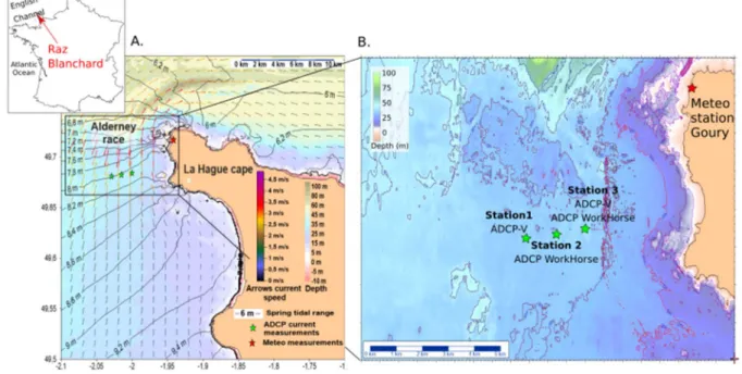
The Alderney Race tidal current is located in the northern part of the Normandy-Brittany Gulf (France) between the Alderney Island and the La Hague Cape (Fig. 1A). Currents are related to the tidal wave coming from the Atlantic Ocean. The tidal wave amplitude increases when it crosses the continental shelf (500 km westward) and subsequently when this wave is reflected by the Cotentin Peninsula, acting as a barrier. This creates a significant tidal range (more than 14 m near the Mont Saint Michel bay) in the Normandy-Brittany Gulf causing strong tidal currents. The maximum tidal range varies from 6 m to 11 m, from North to South of the La Hague Cape (5 km apart). This leads to a significant slope of the water (black contours – Fig. 1A) that generates the strong currents. In addition, the shallow depth (< 50 m, colors Fig. 1A&B) and the presence of the island creates a funnel effect, increasing the flow (arrows on the Fig. 1A). Previous studies mainly focus on numerical models [2] [3] [4]), validated by local and punctual measurements using in situ current meters. They have identified an area with maximum currents velocities [5], located between the La Hague Cape and the Alderney Island (red arrows Fig. 1). In this area, the current magnitude (Umag) can reach 5 m.s-1
during the high spring tides. The tide is commonly described as an asymmetric tide, dominated by a NNE-directed flow current, estimated to be 3 % stronger than the SSW-directed ebb current [6] that are located a bit more to the north. The current direction
is relatively homogeneous in the areas dominated by NNE and SSW directed currents. The current inversion during the transition between tides is relatively fast, around 15 minutes. Because of strong in situ technical constrains for
instrumentation (strong currents, short time window with relatively low currents during the inversion, etc) only few studies have been carried out over long periods.
Fig. 1: A. Location map with simulated tidal amplitude (spring tide), direction of maximum currents, as well as current-measurement locations; B. Zoom on the measurement area showing the location of 3 ADCP stations and the meteorological station.
III. MATERIALS AND METHODS
Since the 21th April, 2017, we have carried out 5 campaigns on the Thalia and Côtes de la Manche research vessel (CNRS-INSU, France) that allowed the measurement of water level and currents along vertical profiles, at three different stations (Fig. 1). These stations are located along an E-W profile and are named respectively stations 1, 2 and 3 (from West to East). They are located south of the strongest current zone for technical constraints, particularly the difficulty to find plane areas (rocks with one meter mean size). We deployed on the bottom (made of boulders and blocks) one structure for each station, where ADCP (Accoustic Doppler Current Profiler) have been fixed. These structures have been designed specifically to resist to strong currents and to protect the sensors from possible impacts of pebbles or other particles, moving close to the bottom (bottom mainly consists of sand and pebble [7]. The maximum immersion depth was around 40 m. Technical problems occurred related to the recovery of the structures with an automatized remote buoy and the huge amount of data recorded (up to 107 days of data corresponding to ~20 million entries in the database). Since the last campaign took place from mid-October 2017 to February 2018, these last data are still in processing. We have also collected meteorological (Goury semaphore, Météo France) and wave parameters (French buoy network Candhis) in open access sources in order to complete our database.
A. Tidal currents and elevation
Pressure sensors from the ADCP allow the measurement of the surface variations above each offshore structure.
Measurements of currents along vertical profiles using ADCP have been carried out simultaneously for the three structures in the three locations (Fig. 1). During a typical campaign at sea, we have recovered the structures, collected the data and re-immersed the structures. During each data recovery, we checked if the ADCPs were still operating. The measurement cells size is 1 m high and the first cell is located from 1.5 to 2 m above the sea floor.
We used two different types of ADCP models from RDI®: i) an ADCP-V 500 kHz and ii) an ADCP Workhorse 600 kHz. The model of ADCP deployed in each station and their acquisition frequency varies through time because of one accidental lost and adjustment of the acquisition frequency according to the batteries and memory capacity (Table 1). The station 1 has been equipped with an ADCP-V. In station 2, an ADCP Workhorse has been used. In station 3, an ADCP-V has been initially installed from April to June 2017. This sensor has been lost and replaced from September to October 2017 by an ADCP Workhorse.
TABLE 1:ADCP CONFIGURATIONS FOR THE THREE MEASUREMENTS STATION DURING THE YEAR 2017(STATION LOCATED IN FIG.1)
The ADCP-V (station 1) were configured to take two measurements per second (2 Hz) during 20 minutes every hour for wave analysis, and one measurement per second (1 Hz) during one minute every five minutes (Table 1). During the first acquisition period from April to June 2017, the ADCP Workhorse in the station 2 have first been configured to calculate the average current over periods of five minutes with one measurement per second (Table 1). During the second acquisition period from September to October 2017, the both ADCP Workhorse have been configured to take one measurement per second (station 2 and 3). Because of the lost in station 3 during the first period, in this paper, we present only the data from stations 1 and 2.
Each ADCP measures the current velocity along three axes, directed north-south (V, positive values northward), east-west (U, positive values eastward) and vertically (W, positive values upward) for each point, along vertical profiles. The two main velocity components (U and V) allow the calculation of the velocity vectors (Umag). The direction ranges from 0 to 360°,
with 0° northward. The data were averaged over a period of 5 minutes (ܷതതതതതതത) to allow easy viewing and to study the velocity
evolution during tidal cycles (Fig. 3, Fig. 4 and Fig. 5). The high-frequency raw data (1 Hz and 2 Hz) are presented at the end of this paper (Fig. 6).
The current asymmetry has been also studied using the asymmetry coefficient according to the following equation [8]:
ܽ ൌಹƲ
ಽƲ (1)
with UHT, the mean Umag during the high tide phase defined on
the Fig. 3C and ULT, the mean of Umag on the low tide phase. On
the same phases, the direction asymmetry has been also calculated with [9]:
οߠ ൌ ȁߠு்െ ߠ்െ ͳͺͲιȁ (2)
with ߠு் the mean direction during the high tide phase and ߠ்
the mean direction during the low tide phase.
After this general analysis, the vertical velocity profiles have been compared for eight cases of Umag averaged on the water
column to study the variability of profiles [10]. This analysis of profile shape has been made by using the equation:
ܸሺݖሻ ൌ ܸቀ௭ௗቁ ଵ ఈΤ
(3)
which allows to analyzed the variability of the Į coefficient and where V0 corresponds to the surface velocity, d represent the
depth of the water column and z the distance from the bottom for each point. The use of this method could be discussed, as the higher measuring cell of the ADCPs is located at 3 m above
the surface. The Į coefficient have been tested for a range of values from 1 to 15, for each intervals of 0,1 and the best coefficient have been estimated from linear regression fit of LogLog representation of velocity. This analysis takes into account the velocity variations in the boundary layer accurately for important depths. According to [8] and [11], the boundary layer may extend over tens of meters in high hydrodynamic conditions.
B. Waves data
For the wave analyses, we have collected open source data from the buoy located 20 km North of Bréhat (Candhis network). The ADCP-V (initially station 1 and 3 and then only station 1 – Fig. 1), allowed the calculation of the main waves parameters, using different methods: Hs (significant height), Ts (significant period) and Dp (main peak direction). We chose the orbital velocities method. According [12], this method is assumed to be reliable, especially when the free surface spectral analyses cannot be done, which is the case in the present paper, due to pressure sensor problems.
C. Wind intensity and direction
The wind data used in this study are provided by the Météo-France semaphore in Goury (Fig. 1). Each data corresponds to an average over a period of 6 minutes, at an altitude of 10 m. The wind direction has been measured with a resolution of 10°.
I. PRELIMINARY RESULTS
A. General meteorological and waves climates during campaigns
One main wave regime has been identified from both Bréhat and our data set (Fig. 2A&B.), with waves coming from the West (N280°-N290°).
A secondary wave regime has been found in the Bréhat data (Fig. 2A), from the north and on our data (Fig. 2B) coming from the northeast but is negligible compared to the main regime. The dominant wind comes from the southwest (from N180° to N270°) and less frequently from the east (Fig. 2C). The waves from the principal regime come from the Atlantic Ocean where the fetch length is very large. In the other directions, the fetch length is not enough important to generate a significant waves. The directions show a more important dispersion from the southwest to northwest compared with Bréhat. This could be due to wave refraction on the islands or due to shallower depth. During the acquisition campaigns, five neap/spring tide cycles have been recorded. The tidal range fluctuated between 1.8 m to 7.8 m (Fig. 3A), the averaged speed wind reached 16 m.s-1
and the maximum Hs was 4.3 m at Bréhat and 3.5 m at our study area (Fig. 3A).
A. Current evolution during a typical tide cycle
The evolution of current velocities in the Alderney Race area follows a progressive tidal wave regime. The maximum velocities are recorded during the high and low tide and not during the flood and ebb, (Fig. 3B.). One typical tidal cycle is showed in Fig. 3C.
Fig. 2: Waves and wind climates during the field works: A. Waves origin according to the significant height (Hs) for the Bréhat station (~110 km Southwest of Alderney Race) and B. station 1 (location Fig.1); C. Wind origin from the Météo-France measurements in Goury semaphore.
Fig. 3: A. Times series of the conditions evolution during the field work: top, water level evolution; middle, significant wave height (Hs, Bréhat station and ADCP-V data; station 1) and bottom, wind intensity. B. Spatial-temporal diagrams of the Umag (top) and direction (bottom) during the first neap/spring tide
A first current velocity peak is registred during the high tide with an averaged direction toward the NNE (~N20°) for the three stations Subsequently, the velocity decreases during the first half of the ebb until it reaches a value close to 0.1 m.s-1
(Fig. 3B). Current velocities increase again progressively in the opposite direction, toward the SSW (N190°) until the low tide, when a second velocity peak is recorded. Then the current velocities decrease until the half flood and a new tidal cycle start. The current inversions in the tide cycle is characterized by quasi-instantaneous clock-wise current rotation. The maximal mean Umag recorded are correlated with the tidal range
(Fig. 3B.). In the area, the highest measured of mean Umag over
the water column reaches 3 m.s-1 during the high tide with the
higher tidal range of 7.8 m (data averaged for 5 minutes). In neap tide conditions (tidal range < 1.8 m), the velocities during the high tide are relatively lower, around 1.8 m.s-1. As shown in
Fig. 1, the measurement site is located to the south of the maximal current zone of Alderney Race. However, during the acquisition period, and for all winds, waves and tides conditions, Umag during high and low tide is always higher than
1 m.s-1.
B. Tide asymmetry
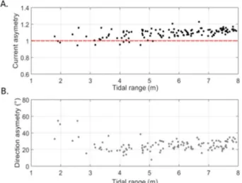
The spatial-temporal diagram Fig. 3B and the graph Fig. 5A, clearly show an asymmetric tide, with higher velocities during the high tide compared with the velocities during low tide. The asymmetry coefficient a defined by (1) ranges from 0.9 to 1.2, between high and low tide phases (Fig. 4A). When this coefficient is lower than 1, the mean intensity of Umag is higher
during low tide relatively to the high tide. In opposite, when this coefficient is higher than 1, the intensity of Umag is higher
during high tide relatively to the low tide. In some cases, for tide range less than 5 m, the intensity of Umag is higher during
low tide relatively to the high tide.
Fig. 4: A. Current asymmetry coefficient (with red line a = 1); B. Direction asymmetry
In most of the other cases and for tidal ranges higher than 5 m, the high tide mean velocity is higher than for the low tide, as shown by the asymmetry. For higher tidal ranges, the asymmetry increases as the tidal range increase.
Concerning the direction (asymmetry defined by (3)), the flow is not bidirectional and the result shows a significant angle between the high and low tides current directions (Fig. 4B). The mean deviation equals 25° but it may increase to 50° for low tidal ranges (below 3 m).
C. Vertical profile variations during different tide phases
Firstly, the Į coefficient have been calculated, using five minutes averaged data windows. However, when Umag is lower
than 0,5 m.s-1 for all the water column, the associated profiles
are relatively linear and this induces high values for the Į coefficient (for 0.2 m.s-1 the Į coefficient is up to 15, Fig. 5).
Therefore, we removed all the profiles when Umag is lower than
0,5 m.s-1 for the calculation of the average of the Į coefficient.
This gives an average value equals to 6.6 ranging from 4 to 12, as in the study of [9].
In a second step, we have studied the relationships between the shape of the vertical profiles and the averaged velocity in the water column. We chose eight different cases for eight different averaged velocities (0.2; 0.5; 1; 1.3; 1.5; 2; 2.5 and 3 m.s-1,
Fig. 5). The selection criteria in Fig. 5 where the Umag averaged
equal to the defined velocity at more and less 3 % (gray envelop). Then, all the profiles have been merged and the Į coefficient have been calculated (table Fig. 5). The graph in Fig. 5 shows that for a given averaged velocity, all the profiles display a relatively similar shape, but the variability of Į is too important to infer a correlation. In addition, there is no direct apparent relationship between the Į coefficient and the increase of Umag (Fig. 5).
During a third step, we calculated the average for the Į coefficient only in windows of 15 minutes during the different tide phases and specially around the velocity peak during high and low tide. This gives a value of 7.4 for the coefficient during high tides and value of 8.3 for the low tides. This difference between the Į values indicates a more bended profile and a more developed boundary layer for high tides compared with low tides. Such tendency is corroborated by the analyses of the velocity gradients between the sea bed and the surface, showing stronger gradient during high tide and more generally, when the velocity increases.
Fig. 5: In gray, all profiles from the database for eight mean velocity (values indicated in table). In black: averaged vertical profiles for these different Umag. In
table, the different cases and the Į coefficient corresponding
D. Preliminary observations on the waves/current interaction
During the acquisition period of September to October 2017, our data from the ADCP configured to 1 Hz frequency for acquisition, allows the visualization of the waves influence in the water column (Fig. 6). Two cases are presented here: the 27th and 30th September cases showing a tidal range of 3.4 m
and 2.6 m (see Table 2 and Fig. 3).
TABLE 2:CHARACTERIZATION OF EVENTS DESCRIBED AND PRESENTED FIG.6
During the first case, the significant wave heights reaches only 0.5 m, while Hs reaches 1.5 m, during the second event (Table 2). For these events, waves are coming from the northwest (N290°). For each case, we have selected two periods of 5 minutes showing two different current velocity situations, with averaged velocities ܷതതതതതതതof 1.3 m.s -1 and 0.2 m.s-1. This
selection of four events allows the comparison of different wave heights (0.5 m and 1.5 m) for the same current situation (for 1.3 m.s-1 or for 0.2 m.s-1) and the comparison of different
current velocities (1.3 m.s-1 and 0.2 m.s-1) for the same wave
height (for 0.5 m and for 1.5 m) (Table 2). Three chosen events correspond to low tide phases with a main current direction toward the SSW and one event to high tide phase with a main current direction toward the NNE (case 30/09 with ܷതതതതതതത of
0.2 m.s-1).
Fig. 6 summarizes the Umag and direction evolutions using
spatial-temporal diagrams (during 5 minutes) for the four selected events. The velocity distribution using histograms at four selected depth (33 m, 23 m, 13 m and 3 m above the sea floor) is also represented for each event, the red and blue histograms correspond to high (1.5 m) and low (0.5 m) Hs, respectively. Different color scale for current velocities are used
for the event with a low ܷതതതതതതത(0.2 m.s-1) and for the event with
a high ܷതതതതതതത (1.3 m.s -1).
For the low current velocity events (ܷതതതതതതത = 0.2 m.s-1), the mean
velocity profiles (Fig. 5) shows that ܷതതതതതതത only slightly varies
in the water column. However, in details, the wave effect is clearly highlighted by Umag variations in the upper part of the
water column (Fig. 6A) for the event with relatively high Hs (1.5 m). In this case, Umag recorded between two profiles at 1 Hz
vary from 0 to 0.8 m.s-1. Increasing Umag (> 0.5 m.s-1) in the
upper water column corresponds to the wave propagation. The direction variations (Fig. 6A) are very significant for this case with an angle up to 100° between two profiles separated by few seconds. The flow direction is mainly striking toward the SSW but some local and brutal changes related with the waves occur, toward the SSE. A period of 8.5 s can be calculated and the structures related with the waves are well defined. In these environmental conditions, waves have an important impact on the current. For the event with small Hs (0.5 m), the Umag
variation is lower with recorded variations of about 0.5 m.s-1
between two profiles (in a few seconds). However, oscillation structures are still visible in the spatial-temporal diagram, meaning that the impact of waves in the water column for significant height of 0.5 m is not negligible when the mean tidal current is low (0.2 m.s-1). These observations are confirmed by
the distribution of current velocity on the histogram (Fig. 6). The histogram distribution near surface at 23 and 33 m above the bottom is wider for the event with high Hs compared with low Hs. This spreading decreases with depth and the distribution becomes more focused on the mean velocity. This mean velocity is centered on 0.1 m.s-1, while it is expected to be
centered on 0.2 m.s-1. It may be explained by the fact that the
mean velocity calculated at 0.2 m.s-1 take account the low
acceleration for waves propagation [13].
For the high current velocities events (Fig. 6B), the upper water column displays several structures related with rapid variations of current velocities. These structures are well defined when Hs is high (1.5 m case) and less defined when Hs is low (0.5 m case). For these events, Umag recorded between two profiles at
1 Hz vary from 0 to 0.9 m.s-1 occurring in few seconds. For the
high current velocity event with low Hs (ܷതതതതതതത = 1.3 m.s-1and
compared with the events with low current velocities (0.2 m.s-1
events), with only a direction variation of 30° (N180 – N210, toward the SSW). This means that the current directions mainly reflect the tidal influence and not the wave effects, as the tidal currents during the low tide are focused toward the SSW. In the case of high Hs (1.5 m), homogeneous oscillations appear and affect the entire water column up to the deepest ADCP measuring cell. The period of these oscillations has been calculated and equals 6.6 s. At surface, Umag recorded between
two profiles at 1 Hz vary from 0.7 to 2.1 m.s-1. In both cases,
with low (0.5 m) and high (1.5 m) Hs, the histogram distribution are centered on mean velocity values that decrease with depth, following a power law, as shown in Fig. 5. The histogram distribution of the upper measuring ADCP cell, near the surface
is relatively wider (red curve) when Hs is high compared with the case of low Hs. This shows that waves with a height of 1.5 m are able to affected the upper water column, even when the tidal current are relatively high (1.3 m.s-1).
Other structures are found at depth (arrow on the Fig. 6B) and probably initiated on the sea floor and thus may be assumed as turbulent structures associated with the bottom roughness. The clearer example of turbulent structures is found the 27th
September for high ܷതതതതതതത (1.3 m.s-1), during the first minute of
acquisition (arrows on the Fig. 6B). This structure may be up to 20 m in width, with an irregular shape and possibly affects up to 30 % of the lower water column.
Fig. 6: Data for the four studied cases: two events with different current velocity situations are selected during 5 minutes: A. ܷതതതതതതത = 0.2 and B. 1.3 m.s -1. For each
case, two moderates waves climate (Hs = 0.5 m and Hs = 1.5 m) are presented. The spatio-temporal diagrams on the top of Fig. 6A&B are the Umag and the
II. CONCLUSION AND PERSPECTIVES
Three ADCP have been deployed in the Alderney Race area during fives neap/spring tide cycles. These data, which cover a long-time period allow the study of the current evolution at 1 Hz for several cycles of neap/spring tides. This paper describes preliminary results concerning:
i) The evolution of the asymmetry coefficient according to the tidal range and an inverse asymmetry during specific events. ii) A significant deviation of current directions occurs between the high and low tides phases (up to 60° during low tidal range) at our measurement site. According to [13], a current deviation between 10 to 30° can affect the efficiency of tidal turbines. iii) An estimation of the Į coefficient of 6.6 for all periods of measurement with a difference between the high and low tide phases. This value is close to the Į coefficient recommended in the literature [14].
iv) An important variability for the average velocity along vertical profiles (variations of Umag from 0.7 to 2.1 m.s-1 in few
seconds) that may be attributed to the tidal range, to the stage of tide, to the roughness of the sea floor, to the wind or the waves.
v) A preliminary description of four events showing two different types of structures: an oscillation of the water particles linked with the waves in the upper part of the water column (but sometimes reaching the bottom) and turbulent structures probably linked with the roughness of the sea floor.
In a future work, we will quantify the influence of the waves on the tidal currents and the influence of the tidal currents on the orbital velocity of waves mainly in the cases of high currents and high waves. The important database collected allows us to study these processes for many events that will be presented in the future. In addition, the influence of the wind intensity and direction on the current characteristics will be also developed in future studies.
ACKNOWLEDGMENT
Authors are supported by the HYD2M project (ANR-10-IEED-0006-07) funded by the program called “Investissements d’avenir” for the building of France Energies Marines. Authors acknowledge the crews of the ocean research vessels the CNRS vessels “Thalia” and “Côtes de la Manche”.
REFERENCES
[1] Bahaj A.S., Myers L.E., “Analytical estimates of the energy yield potential from the Alderney Race (Channel Islands), using marine current energy converters”, Renewable Energy, vol. 29, pp 1931-1945, 2004. [2] Bailly du Bois P., Dumas F., “Fast hydrodynamic model for medium- and
long-term dispersion in seawater in the English Channel and southern North Sea, qualitative and quantitative validation by radionuclide tracers”, Ocean Modelling, vol.9, pp 169-210, 2005.
[3] Neill S.P., Jordan J.R., Couch S.J., “Impact of tidal stream turbines on sand bank dynamics”, World Renewable Energy Congress, Linköping, Sweden, pp2238-2245, 2011.
[4] Coles D.S., Blunden L.S., Bahaj A.S., “Assessment of the energy extraction potential at tidal sites around the Channel Islands”, Energy, vol. 124, pp. 171-186, 2017.
[5] Bailly du Bois P., Dumas F., Solier L., Voiseux C., “In-situ database toolbox for short-term dispersion model validation in macro-tidal seas,
application for 2D-model”, Continental Shelf Research, vol. 36, pp. 63-82, 2012.
[6] Thieb
[7] Foveau, A., Haquin S., Dauvin J., “Using underwater imagery as a complementary tool for benthos sampling in an area with high-energy hydrodynamic conditions”, Journal of Marine Biology Oceanography, vol. 6, pp. 1–7, 2017.
[8] Thièbault, M. and A. Sentchev, “Asymmetry of tidal currents off w. brittany coast and assessment of tidal energy resource around Ushant island”, Renewable Energy, vol. 105, pp. 735–747, 2017.
[9] Gooch S., Thomson J., Polagye B., Meggitt D., “Site characterization for tidal power”, OCEANS 2009, MTS/IEEE Biloxi-Marine Technology for Our Future: Global and Local Challenges, 2009.
[10] Lewis, M., S. Neill, P. Robins, M. Hashemi, and S. Ward, “Characteristics of the velocity profile at tidal-stream energy sites”, Renewable Energy, vol. 114, pp. 258–272, 2017.
[11] Soulsby R.L., “Similarity scaling of turbulence spectra in marine and atmospheric boundary layers”, Journal of Physical Oceanography, vol. 7(6), pp. 934-937, 1977.
[12] Wiberg P.L., Sherwood, C.R., “Calculating wave-generated bottom orbital velocities from surface wave parameters”, Computers & Geosciences, vol. 34(10), pp. 1243-1262, 2008.
[13] Groeneweg, J., and G. Klopman, “Changes of the mean velocity profiles in the combined wave–current motion described in a GLM formulation”, Journal of Fluid Mechanics, vol. 370, pp. 271-296, 1998
[14] Frost C., Evans P.S., Morris C.E., Mason-Jones A., O’Doherty T., O’Doherty D., “The effect of axial flow misalignment on tidal turbine performance”, In Proceedings of 1st international conference on renewable energies offshore, 2014.
[15] Batten W.M.J., Bahaj A.S., Molland A.F., Chaplin J.R., “The prediction of the hydrodynamic performance of marine current turbines”, Renewable Energy, vol.33, pp. 1085-1096, 2008.