Productivity in Construction

READ THESE TERMS AND CONDITIONS CAREFULLY BEFORE USING THIS WEBSITE. https://nrc-publications.canada.ca/eng/copyright

Vous avez des questions? Nous pouvons vous aider. Pour communiquer directement avec un auteur, consultez la première page de la revue dans laquelle son article a été publié afin de trouver ses coordonnées. Si vous n’arrivez pas à les repérer, communiquez avec nous à [email protected].

Questions? Contact the NRC Publications Archive team at

[email protected]. If you wish to email the authors directly, please see the first page of the publication for their contact information.

NRC Publications Archive

Archives des publications du CNRC

This publication could be one of several versions: author’s original, accepted manuscript or the publisher’s version. / La version de cette publication peut être l’une des suivantes : la version prépublication de l’auteur, la version acceptée du manuscrit ou la version de l’éditeur.

Access and use of this website and the material on it are subject to the Terms and Conditions set forth at

Productivity in Construction

Dozzi, S. P.; AbouRizk, S. M.

https://publications-cnrc.canada.ca/fra/droits

L’accès à ce site Web et l’utilisation de son contenu sont assujettis aux conditions présentées dans le site LISEZ CES CONDITIONS ATTENTIVEMENT AVANT D’UTILISER CE SITE WEB.

NRC Publications Record / Notice d'Archives des publications de CNRC:

https://nrc-publications.canada.ca/eng/view/object/?id=52dc96d5-4ba0-40e6-98d2-8d388cba30cd https://publications-cnrc.canada.ca/fra/voir/objet/?id=52dc96d5-4ba0-40e6-98d2-8d388cba30cd

Productivity in Construction

Dozzi, S.P.; AbouRizk, S.M.

NRCC-37001

The material in this document is covered by the provisions of the Copyright Act, by Canadian laws, policies, regulations and international agreements. Such provisions serve to identify the information source and, in specific instances, to prohibit reproduction of materials without

written permission. For more information visit http://laws.justice.gc.ca/en/showtdm/cs/C-42

Les renseignements dans ce document sont protégés par la Loi sur le droit d’auteur, par les lois, les politiques et les règlements du Canada et des accords internationaux. Ces dispositions permettent d’identifier la source de l’information et, dans certains cas, d’interdire la

Productivity in

Construction

S.P. Dozzi, P.Eng. and S.M. AbouRizk, Ph.D., P.Eng. Construction Engineering and Management

Civil Engineering Department University of Alberta

Institute for Research in Construction National Research Council

IRC-P-3547 NRCC 37001 NR16-2411993E ISBN 0-662-21134-0 Ottawa, December 1993

Preface

NRC' Institute for Research in Con-struction i · delighted to be instrumental in bringing thi important gujdebook to the

con-truction profe ional of Canada. Thi CSCE-NRC project i a good example of lhe kind o.f alliance that i increa ingly important in up-port of lhe Canadian construction indu try as it strives to find internationally competitive ways to do bu. ine . The pairing of the counlry ' leading ource for construction technol.ogie with the enior national profe ional

a

ocia-tion in civil engineering ha produced

a

defini-tive . tatement on the ubject of productivity, which I commend to all reader .

G. Seaden, Director General

Foreword

Contractors have often been heard to say, "As long as we are as aggressive and effi-cient as our usual competitors, we will always get our share of work." But in today's market-place, being as efficient as one's neighbour does not suffice. Competition is no longer lim-ited to contractors working in well defined geo-graphical areas. The available work is being sought by firms from other parts of the country or even of the globe.

Canadian competitiveness, or rather the lack of it, has been in the headlines now for several years. For example, a report in the 25 June 1991 issue of The Economist, entitled "A Survey of Canada," claims that:

"In general, the growth of Canadian

produc-tivity is declining; yet

if

Canada is to remain

a wage economy, it has to be a high-productivity one. Annual high-productivity growth, which has been 2.3 % in 1946-73,fell to 0.9% in 1973-90. And the growth of Cana-dian manufacturing productivity has slowed relative to all other members of the Group of Seven rich countries. Cost competitiveness relative to the United States has declined particularly sharply .. .. "

There are also signs of slowed produc-tivity in Canada relative to Japan. Between 1986 and 1990, the productivity of construction labour in Japan increased by 6.6% a year, while Canadian construction productivity rose by only 1.6% .

In response to this dilemma, the Con-struction Division of the Canadian Society for Civil Engineering (CSCE) developed and im-plemented a program with a view to improving productivity. CSCE, with the assistance of the National Research Council, formed an alliance with the Construction Technology Centre At-lantic Inc. (CTCA), according to which CSCE would produce a manual about ways to im-prove productivity and CTCA would organize seminars. Such seminars on productivity im-provement have taken place across Canada since September 1990, usually in collaboration with the local construction association.

The Institute for Research in Con-struction has now decided to draw on the expe-rience gained from the preparation of the manual and presentations, and publish this doc-ument, "Productivity in Construction." I hope that it receives the attention it deserves and that every supervisor of construction projects refers to it frequently for guidance.

Stephen G. Revay, F.EIC, F.CSCE Past President ( 1989-90) CSCE

1

1.1 1.2 1.3 1.4

2

2.1 2.2 2.2.1 2.2.2 2.2.3 2.3 2.3.1 2.3.2 2.4 2.5 2.6 2.6.1 2.6.2 2.6.3 2.6.4

3

3.1 3.2 3.2.1 3.2.2 3.2.3 3.2.4 3.2.5 3.3 3.3.1 3.3.2 3.3.3

ｾ＠

Table of

Contents

Introduction

Productivity: More Achievement

per Resource ... .... 1

What is Productivity? ... 1

Framework for Productivity Improvement in Construction ... 2

Organization of this Publication ... 2

Techniques for

Measur-ing and ImprovMeasur-ing

Productivity at

Construction Sites

Introduction .. ... ... ... .... ... ... .. 5

Measuring and Interpreting Work and Crew Effectiveness ... 5

Field rating ... ... 5

W ark sampling ... 5

Five-minute rating ... 7

Field Surveys ... .. ... ... ... .... 7

Foreman delay survey ... .. ... .. ... 8

Craftsman questionnaire ... ... .. .. . 8

The Method Productivity Delay Model ... ... ... ... 9

Charting Techniques: Crew-Balance Charts ... .12

Simulation Modelling and Analysis ... l2 The basic phases of construction process simulation ... 12

Building a CYCLONE model... ... 12

Experimenting, analyzing, and simulating ... 14

Simulation and productivity ... 15

Human Factors and

Productivity Improve·

ment

Introduction ... ... .. ... .. ... ... 17

Motivation ... ... 17

Motivation and the construction industry ... ... ... ... ... ... 17

Factors affecting motivation ... l8 Motivators ... 19

Demotivators ... ... ... 19

Absenteeism and turnover ... .. 2 1 Human Factors Related to Productivity ... ... 21

The individual as a factor affecting productivity ... .... 21

Physical limitations .. ... ... 22

The learning curve ... ... . 22

3.3.4 3.3.5 3.3.6 3.4 3.4.1 3.4.2 3.4.3 3.4.4 3.4.6 3.5 3.5.1 3.5.2

4

4.1 4.2 4.3 4.3.1 4.3.2 4.3.3 4.3.4 4.4

5

5.1 5.2 5.3 5.3.1 5.3.2 5.3.3 5.3.4 5.3.5 5.3.6 5.3.7 5.4 5.4.1 5.4.2 5.5

6

6.1 6.2 Crews and teamwork .... ... ... 23

Environmental factors ... .. ... .. ... .. 23

Workspace ... 24

Job Site Planning ... ... ... 24

Job site planning considerations ... 24

Temporary electrical service ... .. 24

Temporary heating and hoarding .... .. . 25

Miscellaneous systems ... 25

Offices, lunchrooms, and sanitary facilities ... .. ... ... ... ... 25

Safety Issues ... . 25

Economic impact of accidents ... 25

Safety and productivity ... 25

Measuring Productivity

from the Cost-Reporting

System

Introduction ... .. ... 27

Data Collection and Processing ... 27

Tracking Person-hours instead of Costs in the Cost-reporting System ... 30

Estimated 'percent complete' ... 30

Physical measurement ... ... .. 31

Earned value ... 31

Performance factors ... 31

Cost Reporting and Analysis Using Project Management Software ... 32

Management Issues

Introduction ... ... ... 35

Quality of Supervision ... 35

Material Management. ... 35

Material management steps ... 36

Responsibilities ... 36

Interfaces and their implications for productivity ... 37 Preplanning ... ... ... ... ... . 38 Material control ... ... ... 38 Procurement. ... ... . 39 Material handling ... .... ... ... 39 Constructability ... ... ... .40 A traditional problem ... .41 Constructability concepts ... .41 Change Management ... ... .... .... ..4 J

Conclusion

Macro- Versus Micro-Productivity . .43 Miscellaneous Ideas for Improving Productivity in Construction ... .43

1 Introduction

1.1

Productivity: More

Achievement per

Resource

Economists have been saying it, so have constructors, organized labour- every-body: to remain competitive, we have to produce more for each dollar spent on con-struction. And "we" is everybody - every worker at a job site can contribute to improved productivity.

Productivity issues can be divided into and micro-level. At the macro-level, one deals with contracting methods, labour legislation, and labour organization; at the micro-level, with the management and op-eration of a project, mainly at the job site.

To improve productivity, we must be able to measure it. And we must be able to measure the effect of changes adopted on methods, effort, and systems. The measured values of productivity can then be compared either to those used to compile the estimate or to some production standards. Although no formal industry standards exist in North Amer-ica, many sources of published productivity data, as well as the databases of various com-panies, can serve as production standards.

A number of complex and interdepen-dent factors can influence productivity on a con-Table 1.1 factors seriously impairing construction productivity

Category

Project Conditions Market Conditions

Design and Procurement Construction Management

Labour

Government Policy Education and Training

Factors

Weather variability Material shortages

Lack of experienced design and project management personnel

Large number of changes Ineffective communications Inadequate planning and scheduling Lack of sufficient supervisory training Restrictive union rules

Slow approvals and issue of permits

Lack of management training for super-vision, project management

struction site. A Construction Industry Develop-ment Council task force developed a question-naire of factors impairing construction productivity (CIDC, 1984). It lists seven cate-gories and 95 factors. Table 1.1 lists the most se-rious factors within each of the seven categories. Research findings by social scientists and construction researchers can be con-tentious, due to the difficulty in accounting for the many interdependencies. The impact of such factors as morale and satisfaction may be debatable, but that should not keep us from thinking seriously about improvements in pro-ductivity. (The idea of improved productivity is too important to be allowed to stumble over academic arguments.) Although we may not know the precise effects of many of these fac-tors, we can observe the effects of combina-tions of them.

1.2

What is Productivity?

Many terms are used to describe pro-ductivity in the construction industry: perfor-mance factor, production rate, unit person-hour (p-h) rate and others. Traditionally, productivi-ty has been defined as the ratio of input/output, i.e., the ratio of the input of an associated re-source (usually, but not necessarily, expressed in p-hs) to real output (in creating economic value). To restate this definition for use in the construction industry: labour productivity is the physical progress achieved per p-h, e.g., p-hs per linear metre of conduit laid or p-hs per cubic metre of concrete poured.

The two most important measures of labour productivity are:

• the effectiveness with which labour is used in the construction process;

• the relative efficiency of labour doing what it is required to do at a given time and place.

Examples of the first measure are the labour dollars required to produce a square metre or square foot of living area, or the labour cost of providing one bed in a hospital. Another example is the labour content required, per barrel of output, to build an oil refinery. In these cases, technological innovations or design improvements have the most significant impact because it is the effectiveness with which labour is used in the building process that is being measured.

Contractors and organized labour are, however, more interested in the second mea-sure, the relative efficiency of labour. Exam-ples include the number of square metres of formwork or linear metres of conduit that can be installed per p-h at a given time and place. Labour efficiency is the basis of most tender estimates, as well as the yardstick by which performance is measured and monitored.

For example, it was reported that 837.4 p-hs were required to construct a house in 1930. By 1965, the requirement was re-duced to 283 .2 person-hours. The reduction in p-hs is equal to an impressive average annual growth rate of 3.2%.

It is not surprising that some analysts have tried to explain this as the result of steadi-ly improving labour efficiency. The real im-provement, however, had little to do with improved efficiency but was due to such tech-nological changes as improved construction ex-cavating equipment and the introduction of drywall to replace wet plaster.

When relative growth in labour pro-ductivity was equated with real improvement in labour efficiency, the construction industry was led to believe that no problem in declining pro-ductivity existed. Apparently lack of motiva-tion is not seen as a problem, and the ever frequent financial losses were blamed either on poor estimating or on the impact of accelerated schedule performance. Construction supervi-sors eventually had to face up to reality and admit that labour efficiency has been steadily declining for some time. By accepting the real-ity and trying to understand both the magnitude Figure 1.1 Framework for productivity improvement

Control Data Collection Planning Management Practices \ _System Construction Project \ Labour Motivation Take Feedback/Control Corrective Action/Improve Procurement Scheduling Compare Actual to Estimated Unit

of and the causes behind this decline, the con-struction industry is making strides toward im-proving productivity.

1.3

Framework for

Produc-tivity Improvement in

Construction

Productivity improvement in construc-tion is best understood when the construcconstruc-tion process is visualized as a complete system as shown in Figure 1.1. The system is made up of the construction project to which material, per-sonnel, equipment, management, and money are inputs. They are consumed by the system in the process of producing the construction unit. Control of the system is achieved by col-lecting and processing information about the rates at which production is attained.

To measure input/output, the parame-ter defined as productivity, two types of input to the system are used: the person-hour/unit and the cost/unit. The first focuses only on labour and is used for labour-intensive operations. The second, cost/unit, combines all effects. The productivity of an operation is measured and compared to the values in the estimate or budget.

If the actual productivity does not compare favourably with the estimated values, the input categories affecting productivity in the system- namely material timeliness, labour effectiveness, and management practices-need to be examined.

To improve labour effectiveness, vari-ous factors can be addressed, including motiva-tion, job safety, environmental factors, and physical limitations. Management practices in-clude scheduling, planning, data collection, job analysis, and control. Material timeliness is en-sured by proper procurement scheduling, site layout, and other issues.

1.4

Organization of this

Publication

The purpose of this publication is to introduce the subject of productivity in con-struction. Each topic can be expanded and dealt with in more detail at every level of the construction process. The reader can pursue the topics further by referring to the books and papers listed at the end of each chapter. Some of these documents are cited in the text.

The subject matter, aimed at such con-struction practitioners as project engineers, su-perintendents or foremen, is presented in a format that can be easily read and understood. It gives practitioners the insights needed to gain an appreciation of productivity in

struction. The publication, although an overview of the subject, covers each topic ade-quately and comprehensively.

Acknowledgment

The authors have drawn freely from written contributions to a seminar series jointly sponsored by the Canadian Society for Civil Engineering and the Construction Technology Centre Atlantic Inc. The seminars were enti-tled "Productivity on Canadian Construction Sites: An Overview. What Supervisors Should Know and Do."

The contributors were C. Fear, R. French, J. Gibson, G. Jergeas, K. Lemon, S. Perfect, K. Pressnail, S. Revay, A. Russel, L. Tardif, C. Trembley, L. Waugh, and S.P. Dozzi, who also served as the editor.

Additional Readings

Adrian, J.J. 1987. Construction Productivity

Improvement. New York: Elsevier Science

Publishing Company.

Alfeld, L.E. 1988. Construction Productivity,

On-Site Measurement and Management. New

York: McGraw Hill.

CIDC, 1984. Canada Construction Industry De-velopment Council, 235 Queen Street, Ottawa, Ontario K1A OH5.

Halpin, D.W. 1985. Financial and Cost

Con-trol Concepts for Construction Management.

New York: John Wiley and Sons.

Oglesby, C.H., H.W. Parker, and G.A. Howel. 1989. Productivity Improvement in

Construc-tion. New York: McGraw Hill.

Warren, R.H. 1989. Motivation and

Productivi-ty in the Construction Industry. New York: Van

..

2 Techniques for Measuring

and Improving Productivity

at Construction Sites

2.1

Introduction

The management of site-related issues in construction projects is often complex and difficult. The main problem is the quantifica-tion of all factors involved on site. The most accurate measure of productivity in construc-tion is the number of units produced per per-son-hour (p-h) consumed, or its reciprocal, the number of p-hs consumed per unit produced. The productivity of a process can be measured indirectly by observing the level of activity of its resources.

Work studies and surveys may have a demotivating effect on the workforce. Special precautions must be taken to avoid the percep-tion that the company is spying on its workers. Education and information sessions are recom-mended to create a team approach to productiv-ity improvement. At a micro-level, workers are a valuable source of information concerning their performance or efficiency. Participation by the tradesmen 1 _{or supervisors can be} expect-ed only if requestexpect-ed.

This chapter deals first with proven techniques that are more widely used to mea-sure the effectiveness (and, indirectly, the pro-ductivity) of construction workers and crews. Also discussed is the use of the data collected to improve the productivity of a construction process. A discussion on a method for measur-ing both effectiveness and productivity at the same time, the Method Productivity Delay Model, (Adrian and Boyer, 1976) follows . The second part of this chapter deals with more ad-vanced methods to study and improve the pro-ductivity of a given construction process. With the increased use of computers, simulation is one of the more advanced techniques that could improve productivity. The idea of using sys-tems simulation in planning and analyzing con-struction processes is introduced. To make this as practical as possible, the discussion is limit-ed to the CYCLONE methodology (Halpin and Riggs, 1992) that has been developed specifi-cally for construction operations analysis.

1_{The words, foreman, craftsman, and tradesman, are meant in a gender-neutral sense;}

likewise the word, workmanship.

2.2

Measuring and

Inter-preting Work and Crew

Effectiveness

2.2.1 Field rating

Field rating can be used to estimate crudely the level of activity of a construction operation. The method simply categorizes the observed worker as either "working" or "non-working" and uses the ""non-working" fraction as a measure of effectiveness. To collect a random sample, an observer on site observes the work-ers. Once a sample has been collected, the field rating is calculated as total observations in the "working" category divided by the total num-ber of observations, plus 10% to account for foreman and supervisory activity as follows: Field rating

=

total observations of working/

total number of observations+ 10% The number should be roughly over 60% for a job to be satisfactory. For example, if a foreman made 100 observations of workers and only 40 were classified as working at the time, then the field rating would be 50%, i.e., 40/100 + l 0. The job would, therefore, be con-sidered unsatisfactory. The method does not tell the analyzer anything about the sources of problems or inefficiencies. It merely suggests that there is something wrong.

2.2.2 Work sampling

Work sampling is based on statistical sampling theory and is a slightly more sophisti-cated method than field rating. The basic ob-jective is to observe an operation for a limited time and from the observations infer how pro-ductive the operation is. Statistical sampling theory is applied because the amount of time spent collecting data has to be limited. In addi-tion, the number of workers observed is nor-mally a small sample taken from the entire population of possible observations (every glance at the worker is considered an observa-tion and therefore, every work sample can re-sult in a multitude of observations). Instead of dealing with the whole population, the proce-dure is to collect a sample, analyze it, and build a confidence limit around it.

Work sampling estimates the percent-age of time a labourer is productive relative to

the total time the person is involved in the oper-ation. To accomplish this, the following ap-proach can be adopted:

1. Classify the worker's activity as one of three modes of activity: productive, semi-produc-tive (involved in supporting the main activi-ty), and non-productive.

Note: There are a number of possible varia-tions for this classification and readers can develop their own, once familiar with the concept. Flexibility can be enhanced by ma-nipulating the semi-productive classifica-tion. One can easily define various modes of semi-productive activity, as shown in Table 2.1. For example, support work can be of the form "material handling," "instruc-tion and decision making," "equipment maintenance," and others. However, more than a handful of classifications can make it difficult to collect data on site.

2. Develop a data collection form that will fa-cilitate tallying the observations on site, as shown in Figure 2.1, for example.

3. Take random observations of workers in-volved in a given operation in the field. The observation should indicate the workers' ac-tivity mode, i.e., productive, non-productive, or semi-productive. Random, for all practi-cal purposes, means without any bias as to who is being observed and that each worker will have the same chance of being observed as any other worker.

4. Record all observations on the form. Enter a checkmark under the appropriate mode of activity observed.

5. Add up all the checkmarks under each mode and calculate the percentage of activity. In the example (Figure 2.1 ), the 'percent pro-ductive' is calculated as 4/9 (= 45%), the 'percent non-productive' is 3/9 (= 33%), and the balance of 22%, semi-productive.

Table 2.1 Examples of activity classification

Classification Productive Semi-Productive Non-Productive (equivalent (Direct Work) {Indirect Work) (Delay) classification) (Working) (Support Work) (Non-Working) Description Using trade tools Supporting the Not contributing to

main activity the activity Examples mason laying brick, tradesman getting personal breaks,

labourer mixing material, travelling waiting for equip-mortar, electrician to work location, men! to be fixed, pulling wire, welder taking instructions waiting for more

welding pipe instructions, late

start or early departure

Research indicates that the productive work category should normally be over 30%. Results of different work sampling studies vary from the low of 9.4% at Isle of Grain to a high of 64.4% measured by the National Association of Home Builders Research Foundation in

1973. Other representative samples reported are:

• 32% by the Civil Engineering magazine in 1977, measured at various nuclear power sites

• 34.7% by S.B. Palmater, measured at 13 nu-clear power sites

• 46.5% measured by the University of Texas at random sites.

Improving the productivity of the process involves identifying the current activity rating and the sources of non-productive or semi-productive modes. This can be subjec-tively analyzed and depends heavily on the level of detail of the classification scheme adopted and the project being analyzed. A sample set of recommendations is given in Table 2.2.

Figure 2.1 Sample work sampling

data

collection form

Work Sampling Sheet Project:

Date: Observer:

Notes:

Observation Productive Semi-Productive Non-Productive No. (Direct work) (Support work) (Delay)

1

.J

2

.J

3

.J

4

.J

5

.,[

6

.J

7

.J

8

.J

9

.J

Total 4 2 3 Percentage 45% 22% 33% PRODUCTIVITY IN CONSTRUCTION

--Table 2.2 Sample causes of delay and recommended remedial actions

Causes of Delay

(Excessive percentage of time spent on this factor)

Waiting for instruction Finding material Getting material Personal breaks

Suggested remedial action

(Each of these actions will require a detailed analysis)

Pre-plan and pre-assign work duties. Improve site layout.

Examine material handling and site layout.

Examine human resource management and discipline.

Waiting for equipment repair Use stand-by equipment where possible, pre-plan to reassign crews to other activ-ities, schedule equipment maintenance to keep it in good working condition. Waiting or queuing for service Resolve resource allocation problems,

possibly by balancing the resources. Material handling difficulties

2_{Aithough this seems to be}

a large number, in actual applications, every glance at the work in progress is an observation. Therefore, 384 observations is not excessive.

Improve site layout and address safety concerns.

For work sampling to be effective, the observer must make a large number of observa-tions, a number that must be determined from statistical sampling theory. The minimum number generally accepted is 3842 observa-tions. This number is derived from a sampling error of 5% and a level of confidence of 95%. Tables, nomographs, and computer programs can be used to calculate the required number of observations for different sets of error limit or confidence levels.

Work sampling only attempts to indi-rectly measure productivity. It is difficult to determine the productivity of a carpenter, for example, by observing how many hammer blows it takes to drive a nail.

In decision-making, the results should be viewed with caution and used with discre-tion. They cannot be used to measure real labour efficiency, yet they are extremely useful to gain a better insight into motivation, and at the same time help explain the reasons behind drastic variations in production rates.

2.2.3 Five-minute rating

The five-minute rating technique, un-like work sampling, is not based on statistical sampling theory. The method relies on simply observing an operation for a short time. The observation does not result in a large enough sample to support work sampling. The method does, however, provide some insight as to the effectiveness of the crew and can identify areas where more observation is required.

The following procedure can be used to implement the 5-minute rating technique:

1. Identify the members of the crew to be ob-served and structure a form similar to that shown in Table 2.3, with the crew to be ob-served noted in the column headings and the time of observation listed in the rows of the first column.

2. Observe the crews as they are working. For the observation interval (in Table 2.3 the in-terval equals 5 minutes), determine whether the crew member has been active for over half the interval. If so, mark the observation cell with an "x"; if not, leave the cell empty. 3. Add the "x" observations for the entire table

and divide the sum by the total number of observations. In the example of Table 2.3, 22 observations were positive out of a total of 32; therefore, the effectiveness is 22/32 or 68%.

Table 2.3 Sample five-minute rating data collection form

Time Spreader Screeder Grader Bull-Floater

9:50 X X X 9:55 X X X 10:00 X 10:05 X X X X 10:10 X X 10:15 X X X 10:20 X X X X 10:25 X X Effective observations 6 6 5 5

Total observations= 32 Effectiveness = 22/32 Observed effective = 22 5-Minute Rating = 68%

2.3

Field Surveys

The work sampling methods covered in Section 2.2 measure efficiencies in the site operation, but do not go far enough in identify-ing the leadidentify-ing cause for the inefficiency. For example, work sampling might indicate that a craftsman spent 25% of the time being delayed because the required material was not available. The method cannot, however, pinpoint the real cause of the delay or what can be done to re-duce it.

Field surveys and questionnaires are organized ways of involving the foreman or craftsman in the site evaluation and productivi-ty improvement process. Craftsmen are proba-bly the persons most familiar with their work activity. They can easily identify sources of delay and obstacles in their progress. Likewise, a foreman is the person most familiar with the crew and the problems that restrict improve-ment in their productivity.

---Figure 2.2 Typical FDS form 2.3.1 Foreman delay survey

Problem Causing Area Person-Hours Lost

No. of No. of Total Hours Lost Workers Person- Hours

Foreman Delay Survey (FDS) relies on a questionnaire which is to be filled out by the job foreman at the end of a working day ac-cording to a particular survey schedule, e.g., one work week in each month. The question-naire is primarily meant to identify the number of hours of a day lost due to delays. Most FDSs are divided into rework and delay categories. Once a form has been filled out, the informa-tion is extracted in the form of percentages and action taken to ensure that sources of delays are properly dealt with. A typical FDS form is given in Figure 2.2.

Redoing work (design error or change) Redoing work (prefabrication error) Redoing work (field error or damage) Waiting for materials (warehouse) Waiting for materials (vendor furnished) Waiting for tools

Waiting for construction equipment Construction equipment breakdown Waiting for information

Waiting for other crews Waiting for fellow crew members Unexplained or unnecessary move Other:

Comments:

Made by: Date:

Table 2.4 Sample FDS results Problem-Causing Area

Redoing work (design error or change) Redoing work (prefabrication error) Redoing work (field error or damage) Waiting for materials (warehouse) Waiting for materials (vendor furnished) Waiting for tools

Waiting for construction equipment Construction equipment breakdown Waiting for information

Waiting for other crews

Waiting for fellow crew members Unexplained or unnecessary move Other

Total

Total work in person-hours

P-hs Lost 122 24 52 33 22 12 56 15 12 14 10 20 70 462 5 210 Percentage 2.3 0.5 1.0 0.6 0.4 0.2 1.1 0.3 0.2 0.3 0.2 0.4 1.3 8.9

The results of the survey are converted from p-hs into equivalent percentages andre-ported on a form as shown in Table 2.4. The information on the report sheet will identify concerns that the foremen have with the opera-tion. The example in Table 2.4 reveals that too much time is being spent on redoing work due to design error - 2.3% of the time - and waiting for construction equipment - 1.1% of the time.

The FDS is a relatively low-cost method for analyzing the sources of delay dur-ing construction. It can be easily stylized and implemented. For further details regarding im-plementation of FDS in construction, refer to Tucker et al., 1982.

2.3.2 Craftsman questionnaire

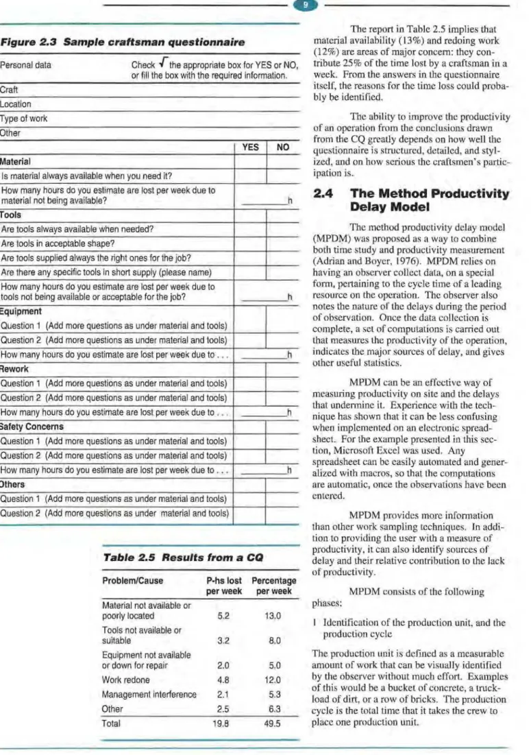
Craftsman questionnaire (CQ) is a questionnaire-oriented technique attempting to address issues and concerns that relate to a craftsman's productivity and motivation. The basic idea is to distribute a simple question-naire, similar to the one shown in Figure 2.3, to craftsmen on a job site to complete. The aim is to identify major factors that inhibit the produc-tivity of craftsmen and estimate the p-hs lost per craftsman per week due to specific causes.

The questionnaire can comprise 50 short questions addressing such areas of con-cern as material availability and site layout, equipment and tool availability, rework items and causes of rework, management interference and inspection, and suggestions for improving the process. In addition, the questionnaire asks for the hours lost per week per craftsman on each area of concern listed. This is often sup-plemented with personal interviews with some of the craftsmen to validate the responses and test the level of seriousness.

Once the questionnaires have been collected, results are compiled and statistics re-ported to all concerned in a form similar to Table 2.5.

---Figure 2.3 Sample craftsman questionnaire

Personal data Check ..[the appropriate box for YES or NO, or fill the box with the required information. Craft Location Type of work Other YES NO Material

Is material always available when you need it?

How many hours do you estimate are lost per week due to

material not being available? h

Tools

Are tools always available when needed? Are tools in acceptable shape?

Are tools supplied always the right ones for the job? Are there any specific tools in short supply (please name) How many hours do you estimate are lost per week due to

tools not being available or acceptable for the job? h

Equipment

Question 1 (Add more questions as under material and tools) Question 2 (Add more questions as under material and tools)

How many hours do you estimate are lost per week due to . . . h Rework

Question 1 (Add more questions as under material and tools) Question 2 (Add more questions as under material and tools)

How many hours do you estimate are lost per week due to ... h

Safety Concerns

Question 1 (Add more questions as under material and tools) Question 2 (Add more questions as under material and tools)

How many hours do you estimate are lost per week due to .. . h

Others

Question 1 (Add more questions as under material and tools) Question 2 (Add more questions as under material and tools)

Table 2.5 Results from a CQ Problem/Cause P-hs lost Percentage

per week per week

Material not available or

poorly located 5.2 13.0

Tools not available or

suitable 3.2 8.0

Equipment not available

or down for repair 2.0 5.0

Work redone 4.8 12.0

Management interference 2.1 5.3

Other 2.5 6.3

Total 19.8 49.5

The report in Table 2.5 implies that material availability (13%) and redoing work (12%) are areas of major concern: they con-tribute 25 % of the time lost by a craftsman in a week. From the answers in the questionnaire itself, the reasons for the time loss could proba-bly be identified.

The ability to improve the productivity of an operation from the conclusions drawn from the CQ greatly depends on how well the questionnaire is structured, detailed, and styl-ized, and on how serious the craftsmen's partic-ipation is.

2.4

The Method Productivity

Delay Model

The method productivity delay model (MPDM) was proposed as a way to combine both time study and productivity measurement (Adrian and Boyer, 1976). MPDM relies on having an observer collect data, on a special form, pertaining to the cycle time of a leading resource on the operation. The observer also notes the nature of the delays during the period of observation. Once the data collection is complete, a set of computations is carried out that measures the productivity of the operation, indicates the major sources of delay, and gives other useful statistics.

MPDM can be an effective way of measuring productivity on site and the delays that undermine it. Experience with the tech-nique has shown that it can be less confusing when implemented on an electronic spread-sheet. For the example presented in this sec-tion, Microsoft Excel was used. Any

spreadsheet can be easily automated and gener-alized with macros, so that the computations are automatic, once the observations have been entered.

MPDM provides more information than other work sampling techniques. In addi-tion to providing the user with a measure of productivity, it can also identify sources of delay and their relative contribution to the lack of productivity.

MPDM consists of the following phases:

1 Identification of the production unit, and the production cycle

The production unit is defined as a measurable amount of work that can be visually identified by the observer without much effort. Examples of this would be a bucket of concrete, a truck-load of dirt, or a row of bricks. The production cycle is the total time that it takes the crew to place one production unit.

ＭＭＭＭＭＭＭＭＭＭＭＭＭＭＭＭＭＭＭＭ

ＭＭ

ｾ＠

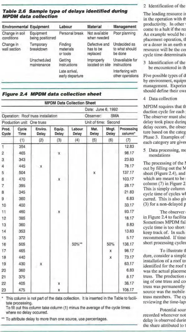
Table 2.6 Sample type of delays identified during

MPDM data collection

Environmental Equipment Labour Material Management

Change in soil Equipment Personal break Not available Poor planning conditions being positioned when needed

Change in Temporary Finding Defective and Undecided as wall section breakdown materials has to be to what should

or tools replaced be done Unscheduled Getting Improperly Unavailable for maintenance instructions located on site instructions

Late arrival, Interfering with early departure other operations

Figure 2.4 MPDM data collection sheet MPDM Data Collection Sheet

Date: June 6, 1992 Operation: Roof truss installation Observer: SMA Production unit: One truss Unit of time: Second

Prod. Cycle Enviro. Equip. Labour Mat. Mngt. Processing Cycle Time Delay Delay Delay Delay Delay column*

(1) (2) (3) (4) (5) (6) (7) 1 354 12.83 2 465 X 98.17 3 343 23.83 4 445 X 78.17 5 504 X 137.17 6 470 X 103.17 7 395 28.17 8 345 21.83 9 360 6.83 10 400 33.17 11 460 X 93.17 12 385 18.17 13 360 6.83 14 353 13.83 15 372 5.17 16 505 50%** 50% 138.17 17 465 X 98.17 18 440 X 73.17 19 430 X 63.17 20 360 6.83 21 375 8.17 22 405 X 38.17 23 475 X 108.17

* This column is not part of the data collection. It is inserted in the Table to facili-tate processing.

To fill out this column take column (1) minus the average of the cycle times where no delay occurred.

** To attribute delay to more than one source, use percentages.

2 Identification of the leading resource The leading resource is that resource involved in the operation with the most impact on the productivity. In other words, the operation will come to a halt if the resource stops producing. An example would be a crane in a concrete placement operation, the mason in brick-laying, or a dozer in an earth moving operation. This resource will be the centre of observation and cycle time determination.

3 Identification of the types of delay that can be encountered in the process

Five possible types of delay include those caused by environment, equipment, labour, material and management. Experience shows that users should define their own types of delay. 4 Data collection

MPDM requires that the observer time the pro-duction cycle for each propro-duction unit placed. The observer must also determine whether a delay took place during a given cycle. If a delay occurs, the observer must indicate its na-ture based on the categories of delays given in Phase 3. Examples of the types of delay under each category are given in Table 2.6.

5 Data processing, model analysis and recom-mendations

The processing of the MPDM data is carried out by filling out the MPDM data collection sheet (Figure 2.4), and Tables 2.7 and 2.8, which are meant to be self-explanatory. First, column (7) in Figure 2.4 has to be completed. This is simply column (1) minus the average cycle time of cycles where no delay has oc-curred. This is also given in Table 2.7, column (3) for a non-delayed production cycle.

The observer can use the form given in Figure 2.4 to facilitate the data collection. Sometimes MPDM fails to work because the cycle time is too short to observe, or too long to keep track of. In such cases, the method is not recommended. If time-lapse film is available, short processing cycles can be captured.

To illustrate the data collection proce-dure, consider a simple process involving the installation of a roof truss. The production unit identified for the roof truss process (Figure 2.4) was the actual placement of a wooden roof truss. The production cycle began with the lift-ing of one truss and concluded when that same truss was permanently braced. The leading re-source was the mobile crane used to place the truss members. The cycle times were timed by reviewing the time-lapse film of the operation.

Potential sources of delay were also recorded whenever noticed. If more than one delay is observed during the same cycle, then the share attributed to the delay should be noted

__________

..

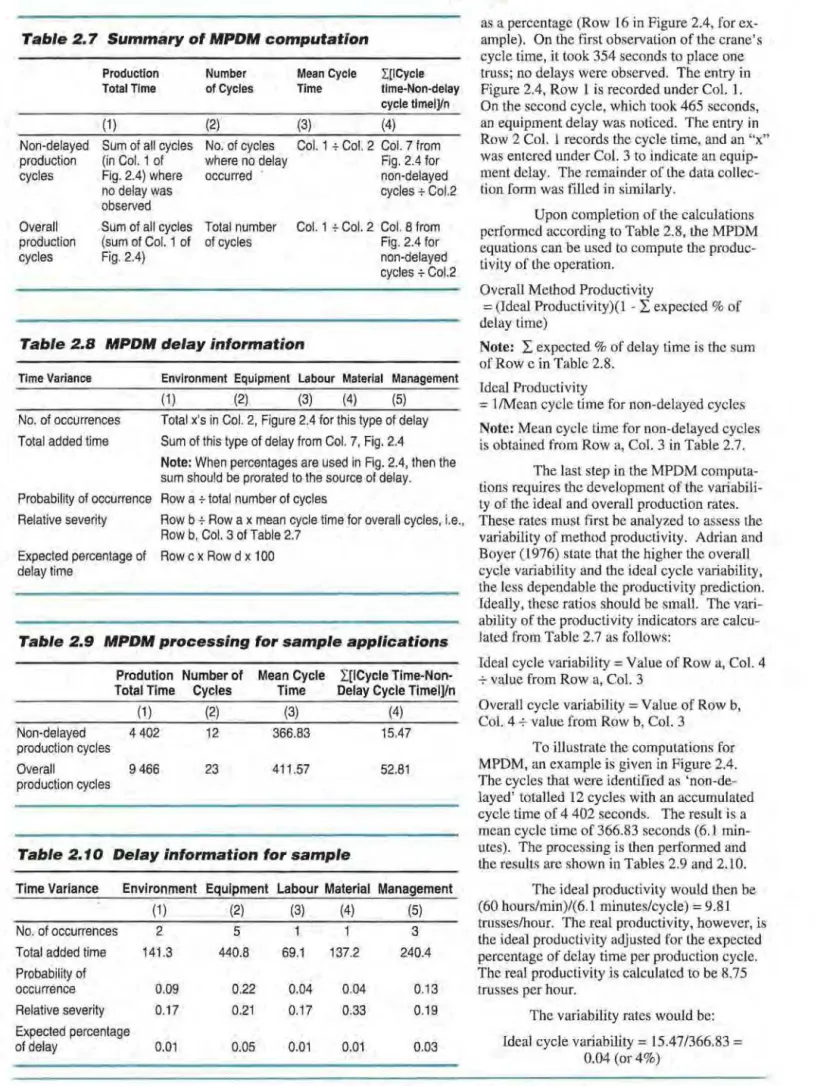
Table 2. 7 Summary of MPDM computation

Production Number Mean Cycle I[ICycle

Total Time of Cycles Time time-Non-delay

cycle timel]/n

(1) (2) (3) (4)

Non-delayed Sum of all cycles No. of cycles Col. 1 + Col. 2 Col. 7 from production (in Col. 1 of where no delay Fig. 2.4 for cycles Fig. 2.4) where occurred · non-delayed

no delay was cycles .;. Col.2

observed

Overall Sum of all cycles Total number Col. 1 .;. Col. 2 Col. 8 from production (sum of Col. 1 of of cycles Fig. 2.4 for

cycles Fig. 2.4) non-delayed

cycles + Col.2

Table 2.8 MPDM delay information

Time Variance Environment Equipment Labour Material Management

No. of occurrences Total added time

(1) (2) (3) (4) (5)

Total x's in Col. 2, Figure 2.4 for this type of delay Sum of this type of delay from Col. 7, Fig. 2.4

Note: When percentages are used in Fig. 2.4, then the

sum should be prorated to the source of delay. Probability of occurrence Row a +total number of cycles

Relative severity Row b + Row ax mean cycle time for overall cycles, i.e., Row b, Col. 3 of Table 2.7

Expected percentage of Row c x Row d x 100 delay time

Table 2.9 MPDM processing for sample applications Prodution Number of Mean Cycle I.[ICycle Time-Non-Total Time Cycles Time Delay Cycle Timel]/n

(1) (2) (3) (4)

Non-delayed 4 402 12 366.83 15.47

production cycles

Overall 9 466 23 411.57 52.81

production cycles

Table 2.10 Delay information for sample

Time Variance Environment Equipment Labour Material Management

(1) (2) (3) (4) (5)

No. of occurrences 2 5 3

Total added time 141 .3 440.8 69.1 137.2 240.4 Probability of

occurrence 0.09 0.22 0.04 0.04 0.13

Relative severity 0.17 0.21 0.17 0.33 0.19 Expected percentage

of delay 0.01 0.05 0.01 0.01 0.03

as a percentage (Row 16 in Figure 2.4, for ex-ample). On the first observation of the crane's cycle time, it took 354 seconds to place one truss; no delays were observed. The entry in Figure 2.4, Row 1 is recorded under Col. 1. On the second cycle, which took 465 seconds, an equipment delay was noticed. The entry in Row 2 Col. 1 records the cycle time, and an "x" was entered under Col. 3 to indicate an equip-ment delay. The remainder of the data collec-tion form was filled in similarly.

Upon completion of the calculations performed according to Table 2.8, the MPDM equations can be used to compute the produc-tivity of the operation.

Overall Method Productivity

=(Ideal Productivity)(l -

2:

expected % of delay time)

Note:

2:

expected % of delay time is the sum

of Row e in Table 2.8. Ideal Productivity

=

1/Mean cycle time for non-delayed cycles

Note: Mean cycle time for non-delayed cycles

is obtained from Row a, Col. 3 in Table 2.7. The last step in the MPDM computa-tions requires the development of the variabili-ty of the ideal and overall production rates. These rates must first be analyzed to assess the variability of method productivity. Adrian and Boyer (1976) state that the higher the overall cycle variability and the ideal cycle variability, the less dependable the productivity prediction. Ideally, these ratios should be small. The vari-ability of the productivity indicators are calcu-lated from Table 2.7 as follows:

Ideal cycle variability = Value of Row a, Col. 4 -;- value from Row a, Col. 3

Overall cycle variability= Value of Row b, Col. 4 -;- value from Row b, Col. 3

To illustrate the computations for MPDM, an example is given in Figure 2.4. The cycles that were identified as 'non-de-layed' totalled 12 cycles with an accumulated cycle time of 4 402 seconds. The result is a mean cycle time of 366.83 seconds (6.1 min-utes). The processing is then performed and the results are shown in Tables 2.9 and 2.10. The ideal productivity would then be (60 hours/min)/(6.1 minutes/cycle)= 9.81 trusses/hour. The real productivity, however, is the ideal productivity adjusted for the expected percentage of delay time per production cycle. The real productivity is calculated to be 8.75 trusses per hour.

The variability rates would be: Ideal cycle variability= 15.47/366.83 =

---

Overall cycle variability= 65.281/411.57 = 0.13 (or 13%)

Such variability is considered to be relatively minor and would indicate that the productivity rates obtained are realistic values.

The results of the analysis can be used to determine what the productivity rate is and what can be done to improve the productivity. Table 2.10 indicates that the most expected delay can occur from equipment (5%), but the most severe (lengthiest) delay has occurred from material. The 22% probability of an equipment delay indicates that management should concentrate on solving the problems as-sociated with equipment.

2.5

Charting Techniques:

Crew-Balance Charts

Crew balance charts are a method of comparing interrelationships among various crew members and equipment required to can)' out a task. This method is applicable to such cyclical tasks as placing concrete.

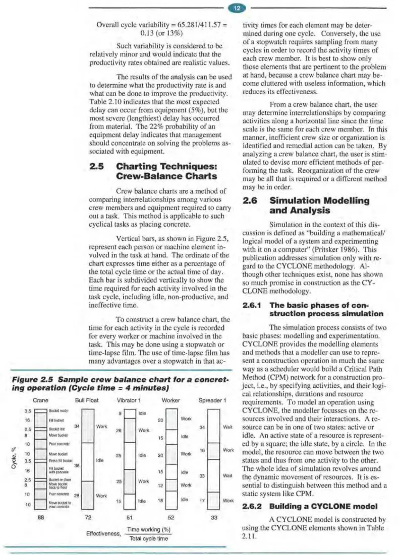
Vertical bars, as shown in Figure 2.5, represent each person or machine element in-volved in the task at hand. The ordinate of the chart expresses time either as a percentage of the total cycle time or the actual time of day. Each bar is subdivided vertically to show the time required for each activity involved in the task cycle, including idle, non-productive, and ineffective time.

To construct a crew balance chart, the time for each activity in the cycle is recorded for every worker or machine involved in the task. This may be done using a stopwatch or time-lapse film. The use of time-lapse film has many advantages over a stopwatch in that

ac-tivity times for each element may be deter-mined during one cycle. Conversely, the use of a stopwatch requires sampling from many cycles in order to record the activity times of each crew member. It is best to show only those elements that are pertinent to the problem at hand, because a crew balance chart may be-come cluttered with useless information, which reduces its effectiveness.

From a crew balance chart, the user may detetmine interrelationships by comparing activities along a horizontal line since the time scale is the same for each crew member. In this manner, inefficient crew size or organization is identified and remedial action can be taken. By analyzing a crew balance chart, the user is stim-ulated to devise more efficient methods of per-forming the task. Reorganization of the crew may be all that is required or a different method may be in order.

2.6

Simulation Modelling

and Analysis

Simulation in the context of this dis-cussion is defined as "building a mathematical/ logical model of a system and experimenting with it on a computer" (Pritsker 1986). This publication addresses simulation only with re-gard to the CYCLONE methodology. Al-though other techniques exist, none has shown so much promise in construction as the CY-CLONE methodology.

2.6.1 The basic phases of con-struction process simulation

Figure 2.5 Sample crew balance chart for

a

concret·

The simulation process consists of two basic phases: modelling and experimentation. CYCLONE provides the modelling elements and methods that a modeller can use to repre-sent a construction operation in much the same way as a scheduler would build a Critical Path Method (CPM) network for a construction pro-ject, i.e., by specifying activities, and their logi-cal relationships, durations and resource requirements. To model an operation using CYCLONE, the modeller focusses on there-sources involved and their interactions. Are-source can be in one of two states: active or idle. An active state of a resource is represent-ed by a square; the idle state, by a circle. In the model, the resource can move between the two states and thus from one activity to the other. The whole idea of simulation revolves around the dynamic movement of resources. It is es-sential to distinguish between this method and a static system like CPM.

ing operation (Cycle time = 4 minutes} Crane 3.5 Bucket ready 16 Fill bucket 2.5 Bucket idle 8 Move bucket 10 Pour concrete 'if< a) 10 Move bucket u _>- 3.5 u ₁₆ Fill bucket with concrete 2.5 Bucket on lloor 8 Move bucket back to floor 10 Pourcoocrete

10 Move bucket to _{pour concrete}

88

Bull Float Vibrator 1 Worker Spreader 1

9 Idle 20 Work 26 Work 15 25 Idle 20 Idle 15 25 Work 12 28 Work 15 Idle 18 72 51 52

Effectiveness, Time working (%)

Total cycle time

Work 34 Idle Work 16 Idle 33 Work Idle ₁₇ Wait Work Wail Work 33

2.6.2 Building a CYCLONE model

A CYCLONE model is constructed by using the CYCLONE elements shown in Table 2.11.

- - -

--The rules for structuring CYCLONE network models using these elements are sum-marized in Table 2.11.

The CYCLONE modelling procedure uses the following steps:

1. Identify all resources involved in the opera-tion to be modelled.

2. Define the tasks (active states of a resource) composing the process to be modelled. Rep-resent them with CYCLONE square elements (a task that is constrained by the availability of more than one resource is represented by a COMBination element and a non-constrained task by a NORMAL element).

3. Define the resource requirement in the tasks and decide where they should wait when a constrained task is not available for service, i.e., it is waiting for other resources before it can proceed. This defines circle elements known as QUEue nodes in CYCLONE ter-minology.

4. Establish the logical relationships between these tasks (i.e., precedence and sequencing of the tasks) by connecting the COMB I, NORMAL, and QUEue nodes with direc-tional flow arrows indicating where the re-source would be moving from and to upon completion of a task. This makes up the CYCLONE network.

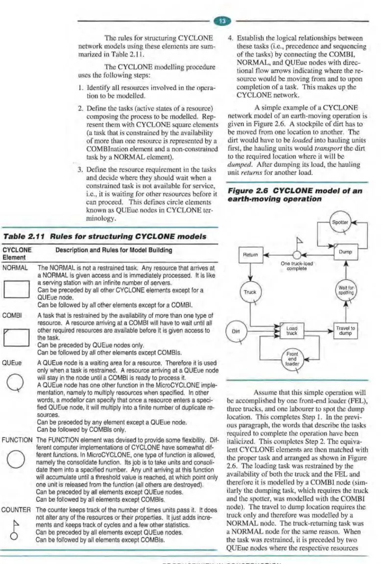
A simple example of a CYCLONE network model of an earth-moving operation is given in Figure 2.6. A stockpile of dirt has to be moved from one location to another. The dirt would have to be loaded into hauling units first, the hauling units would transport the dirt to the required location where it will be

dumped. After dumping its load, the hauling

unit returns for another load.

Figure 2.6 CYCLONE model of an earth-moving operation

Table 2.11 Rules for structuring CYCLONE models CYCLONE Element NORMAL

D

COMB I

D

QUEue

0

FUNCTION

0

COUNTER

Description and Rules for Model Building

The NORMAL is not a restrained task. Any resource that arrives at a NORMAL is given access and is immediately processed. It is like a serving station with an infinite number of servers.

Can be preceded by all other CYCLONE elements except for a QUEue node.

Can be followed by all other elements except for a COMBI. A task that is restrained by the availability of more than one type of resource. A resource arriving at a COMBI will have to wait until all other required resources are available before it is given access to the task.

Can be preceded by QUEue nodes only.

Can be followed by all other elements except COMB Is.

A QUEue node is a waiting area for a resource. Therefore it is used only when a task is restrained. A resource arriving at a QUEue node will stay in the node until a COMB I is ready to process it.

A QUEue node has one other function in the MicroCYCLONE imple-mentation, namely to multiply resources when specified. In other words, a modellor can specify that once a resource enters a speci-fied QUEue node, it will multiply into a finite number of duplicate re-sources.

Can be preceded by any element except a QUEue node. Can be followed by COMBis only.

The FUNCTION element was devised to provide some flexibility. Dif-ferent computer implementations of CYCLONE have somewhat dif-ferent functions. In MicroCYCLONE, one type of function is allowed, namely the consolidate function. Its job is to take units and consoli-date them into a specified number. Any unit arriving at this function will accumulate until a threshold value is reached, at which point only one unit is released from the function (all others are destroyed). Can be preceded by all elements except QUEue nodes. Can be followed by all elements except COMBis.

The counter keeps track of the number of times units pass it. It does not alter any of the resources or their properties. It just adds incre-ments and keeps track of cycles and a few other statistics. Can be preceded by all elements except QUEue nodes. Can be followed by all elements except COMB Is.

Assume that this simple operation will be accomplished by Of!e front-end loader (FEL), three trucks, and one labourer to spot the dump location. This completes Step 1. In the previ-ous paragraph, the words that describe the tasks required to complete the operation have been italicized. This completes Step 2. The equiva-lent CYCLONE elements are then matched with the proper task and arranged as shown in Figure 2.6. The loading task was restrained by the availability of both the truck and the FEL and therefore it is modelled by a COMBI node (sim-ilarly the dumping task, which requires the truck and the spotter, was modelled with the COMBI node). The travel to dump location requires the truck only and therefore was modelled by a NORMAL node. The truck-retuming task was a NORMAL node for the same reason. When the task was restrained, it is preceded by two QUEue nodes where the respective resources

wait. Loading was preceded by the FEL QUEue where the PEL waits until a truck is available. The dirt was modelled with a QUEue node and the truck waiting for loading also with a QUEue node. The truck waiting for the dumping was modelled by another QUEue node. This emphasizes that the state of the re-source is modelled in CYCLONE methodology, rather than the resource itself.

2.6.3 Experimenting, analyzing, and simulating

Once a model has been built, it can be entered into a computer program such as Mi-croCYCLONE for processing and performing the simulation study. The results of the simula-tion study are:

o an estimate for completing the operation o the hourly production rate

o other measures of equipment utilization.

Figure 2.7 presents another model of an earth-moving operation. It is somewhat dif-ferent from the one in Figure 2.6. The model can be used to balance resources, maximize

Figure 2. 7 Another CYCLONE model of an earth· moving operation

Truck queue

Repair crew idle

Excavator idle at position 1

Excavator idle at position 2

productivity or achieve minimum unit cost, as well as to deal with uncertainty and risk.

The operation considered in this model involves earth moving for a sports training facili-ty in a university area. The earth is to be moved from the location of the training facility to the dump location about 3 km away. Two excava-tors remove earth at the job site at two different locations. A number of trucks carry the dirt, dump it, and return for another cycle. The truck would normally wait until one of the excavators is freed up before proceeding for loading. The operation was observed and data collected on the cycle times of the various equipment using a stopwatch. The observer also noted that the trucks break down on almost 5% of the cycles due to overloading (e.g., from flat tires).

The CYCLONE model of the opera-tion was prepared as discussed previously. One main difference is the modelling of truck break-down. The branch corning out of dummy NORMAL node (No. 14) indicates that every time a truck passes this task, it has 5 chances in 1 00 of ending up being tied in the repair task (No. 8); 95 times in 100 it continues in its cycle. Upon repair, it is released back to its original cycle. This is how equipment break-downs are modelled in CYCLONE to simulate actual breakdown in the operation.

Now the model can be entered into Mi-croCYCLONE. The MicroCYCLONE user manual (Halpin, 1990) gives the reader all the required information. The first step is to transfer the graphical model into a written text file in the MicroCYCLONE syntax. The model in Figure 2.7 translates into the file shown in Figure 2.8. Figure 2.8. Simulation input file

NAME 'Earth-Moving' LENGTH 5000 CYCLE 100 NETWORK INPUT

1 COMB I SET 'LOAD @ 1 'FOL 2 3 PRE 2 10

2 QUE 'EXCAVATOR1 IDLE' 3 NOR SET 2 'TRK BACK CYC' FOL 6 4 COMB I SET 3 'LOAD @ 2'FOL 3 5 PRE 5 1 0 5 QUE 'EXACVATOR2 IBLE'

6 FUN COU FOL 14 QUA 1 7 QUE 'TRK QUEUE'

8 COMBI SET 4 'TRUCK REP' FOL 910 PRE 7 9 9 QUE 'REPAIR CREW'

10 QUE SEL LOAD POSITION'

14 NOR SET 5 'TRK BREAKDOWN' FOL 7 10 PRO 0.05 0.95 SEED 101

RESOURCE INPUT

1 'EXCAVATOR' AT 2 FIX 129.38 4 'TRUCKS' AT 10 FIX 50.86 1 'EXCAVATOR' AT 5 FIX 129.38 1 'REPAIR CREW' AT 9 FIX 28 DURATION INPUT SET 1 5 SET2 35 SET3 9 SET 4 60 SET 50 ENDDATA PRODUCTIVITY IN CONSTRUCTION

- - - C»

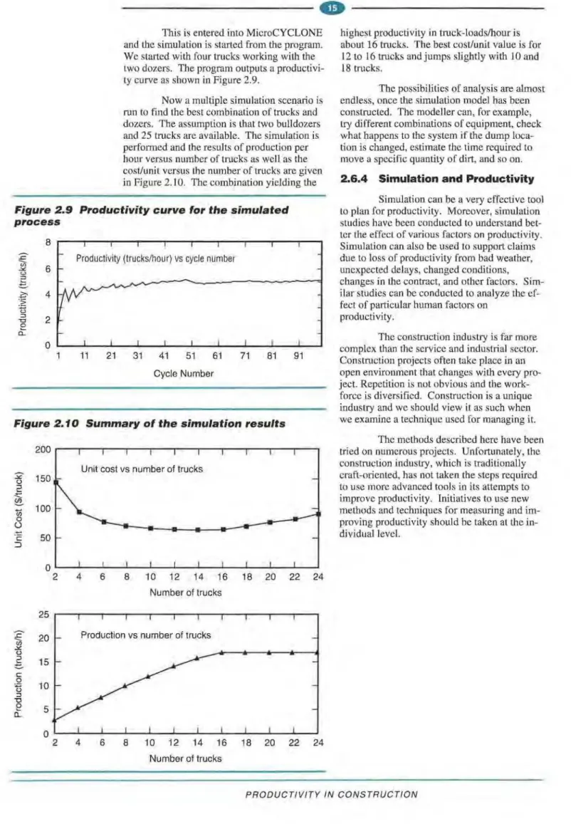
This is entered into MicroCYCLONE and the simulation is started from the program. We started with four trucks working with the two dozers. The program outputs a productivi-ty curve as shown in Figure 2.9.

Now a multiple simulation scenario is run to find the best combination of trucks and dozers. The assumption is that two bulldozers and 25 trucks are available. The simulation is performed and the results of production per hour versus number of trucks as well as the cost/unit versus the number of trucks are given in Figure 2.10. The combination yielding the Figure 2.9 Productivity curve for the simulated process

8

Productivity (trucks/hour) vs cycle number 6

0

11 21 31 41 51 61 71 81 91

Cycle Number

Figure 2.10 Summary of the simulation results

2 () 2 ｾ＠ Cii 0 () 2

--

en ｾ＠ ()

ｾ＠

c: 0

n

_:::J '0

e

c.. 150 100 50 25 20 15 10 5 0

Unit cost vs number of trucks

4 6 8 1 0 12 14 16 18 20 22 24 Number of trucks

Production vs number of trucks

2 4 6 8 1 0 12 14 16 18 20 22 24 Number of trucks

highest productivity in truck-loads/hour is about 16 trucks. The best cost/unit value is for 12 to 16 trucks and jumps slightly with 10 and 18 trucks .

The possibilities of analysis are almost endless, once the simulation model has been constructed. The modeller can, for example, try different combinations of equipment, check what happens to the system if the dump loca-tion is changed, estimate the time required to move a specific quantity of dirt, and so on.

2.6.4 Simulation and Productivity

Simulation can be a very effective tool to plan for productivity. Moreover, simulation studies have been conducted to understand bet-ter the effect of various factors on productivity. Simulation can also be used to support claims due to loss of productivity from bad weather, unexpected delays, changed conditions, changes in the contract, and other factors. Sim-ilar studies can be conducted to analyze the ef-fect of particular human factors on

productivity.

The construction industry is far more complex than the service and industrial sector. Construction projects often take place in an open environment that changes with every pro-ject. Repetition is not obvious and the work-force is diversified. Construction is a unique industry and we should view it as such when we examine a technique used for managing it.

The methods described here have been tried on numerous projects. Unfortunately, the construction industry, which is traditionally craft-oriented, has not taken the steps required to use more advanced tools in its attempts to improve productivity. Initiatives to use new methods and techniques for measuring and im-proving productivity should be taken at the in-dividual level.

ＭＭＭＭＭＭＭＭＭＭＭＭＭＭＭＭＭＭＭＭＭ

ｾ＠

---Additional Readings

Adrian, J. and L.T. Boyer. 1976. "Modeling

MeU10d- Productivity." ASCE J. Const. Div.

103 (3):154-168.

Halpin, D.W. 1977. "CYCLONE: Method for

Modeling of Job Site Processes." ASCE J.

Const. Div. 103 (3):489-499.

Halpin, D.W. and R.W. Woodhead. 1976.

De-sign of Construction and Process Operations.

New York: John Wiley and Sons.

Halpin, D.W. 1990. MicroCYCLONE User's Manual. Division of Construction E ngineering and Management, Purdue University, West Lafayette, Indiana.

Halpin, D.W. and L.S. Riggs. 1992. Planning

anti Analysis of Construction Operations. New

York: John Wiley and Sons.

Pritsker, A. J 986. Introduction to Simulation

and SLAM II. New York: John Wiley and Sons. Tucker, R.L., D.F. Rogge, W.R. Hayes, and

F.P. Hendrickson. 1982. "Implementing

Fore-man Delay Surveys." ASCE J. Const: Div. 108

(4):577-591.

3

Hu111an Factors and

Productivity l111prove111ent

3.1

Introduction

The motivation of workers can be en-hanced through job enrichment (increasing the things that satisfy workers about a job) and by lessening the demotivators (the things that workers dislike). Reducing demotivators only, the predominant practice of North-American management, is not enough; it should be sup-plemented with job enrichment.

Workers are motivated by completing productive quality work, creating or building something, and social relations at work. Pro-ductive work can be produced by good plan-ning and communications. Satisfactory social relations are simply working with other work-ers who are friendly and respectful. Individuals and organizations need goals to try to meet or exceed. Workers can often be motivated through goal-setting. Goals must be clearly es-tablished to elicit maximum performance and provide a feeling of maximum individual achievement. Individuals need a system or method by which to measure their achieve-ments and compare their standings against a given target.

Construction work is varied, which can be satisfying. Workers are often motivated because they see the progress and results of their work. There are also many demotivators. The most common include:

• non-availability of the right material, tools, or equipment

• poor relations between workers and man-agement

• poorly organized projects • breakdown in communication

• lack of recognition of outstanding efforts • disrespectful treatment

• unfair work assignments

• incomplete engineering/design work • lack of cooperation between different crafts • poor supervision

• rework

• no participation in the decision-making process

• restrictive or burdensome procedures. Worker satisfaction and motivation can be increased by removing or reducing these problems. Questionnaires of the type described in Chapter 2 and suggestion boxes can be use-ful in bringing these problems to the surface.

3.2

Motivation

When applying motivational theories to everyday problems, three questions arise:

• What energizes human behaviour? • What directs such behaviour? • How is this behaviour sustained?

The answers given by various social scientists have been expressed in different words; nevertheless, they all seem to agree that human beings are energized by their physiolog-ical needs, and that their behaviour is directed by their expectations and sustained by obtain-ing just reward.

3.2.1 Motivation and the construc· tion industry

The July 10, 1980 issue of The

Listener, a magazine published by the British

Broadcasting Corporation, contained an article describing the British experience in construct-ing nuclear power plants. The followconstruct-ing is an excerpt from that article:

"In recent years, no big plant has been put up on time. No big plant now being built is on schedule. The delay ranges from two to two and a half years for a chemical plant to four years for something as big as Grain (Nuclear Power Plant, Isle of Grain, G.B.). The rot is not solely or even mainly due to strikes; it is the result of almost unbelievably low levels of productivity. Do you believe that a man can spend eight hours on a site but do only 45 minutes' work in the whole day? No? But he can, and this is how they do it. In a standard eight-hour day, clocking on, walking to and from the job, tea-breaks, bad weather, union business, leave less than four hours available for actual work. Inefficiency, overmanning, and other bad habits will eat into another two or more hours, and you are left on a good British site with, at best, one hour and 40 minutes of actual working-time. On a bad site, where ten-minute tea-breaks have been known to stretch to an hour, the figure comes down to 40 minutes. Shop stewards can tell tales of awkward jobs that take hours to set up or high chimneys that take half an hour to climb up and thus ex-plain away the little time a man spends with tools actually in his hands. There is, how-ever, only one such chimney at the Grain.