Robust Vehicle Counting with Severe Shadows and Occlusions

HAL Id: hal-01592042

https://hal.archives-ouvertes.fr/hal-01592042

Submitted on 22 Sep 2017

HAL is a multi-disciplinary open access

archive for the deposit and dissemination of

sci-entific research documents, whether they are

pub-lished or not. The documents may come from

teaching and research institutions in France or

abroad, or from public or private research centers.

L’archive ouverte pluridisciplinaire HAL, est

destinée au dépôt et à la diffusion de documents

scientifiques de niveau recherche, publiés ou non,

émanant des établissements d’enseignement et de

recherche français ou étrangers, des laboratoires

publics ou privés.

Robust Vehicle Counting with Severe Shadows and

Occlusions

Paul Valiere, Louahdi Khoudour, Alain Crouzil, Dung Nghi Truong Cong

To cite this version:

Paul Valiere, Louahdi Khoudour, Alain Crouzil, Dung Nghi Truong Cong. Robust Vehicle Counting

with Severe Shadows and Occlusions. 5th IEEE International Conference on Image Processing Theory,

Tools and Applications (IPTA 2015), Nov 2015, Orléans, France. pp. 99-104. �hal-01592042�

O

pen

A

rchive

T

OULOUSE

A

rchive

O

uverte (

OATAO

)

OATAO is an open access repository that collects the work of Toulouse researchers and

makes it freely available over the web where possible.

This is an author-deposited version published in :

http://oatao.univ-toulouse.fr/

Eprints ID : 16856

The contribution was presented at IPTA 2015 :

http://www.ipta-conference.com/ipta15/

To cite this version :

Valiere, Paul and Khoudour, Louahdi and Crouzil, Alain

and Truong Cong, Dung Nghi Robust Vehicle Counting with Severe Shadows

and Occlusions. (2016) In: 5

IEEE International Conference on Image

Processing Theory, Tools and Applications (IPTA 2015), 10 November 2015 -

13 November 2015 (Orléans, France).

Any correspondence concerning this service should be sent to the repository

administrator: staff-oatao@listes-diff.inp-toulouse.fr

Robust Vehicle Counting with Severe Shadows and

Occlusions

Paul Valiere

, Louahdi Khoudour

, Alain Crouzil

and Dung Nghy Truong Cong

Consort NT Company

65 rue d’Alsace Lorraine, 31000 Toulouse, France e-mail: paulvaliere@gmail.com

2

CEREMA : Centre d’´etudes et d’expertise sur l’environnement, les risques, la mobilit´e et l’am´enagement 1 avenue du Colonel Roche 31400 Toulouse, France

e-mail: louahdi.khoudour@cerema.fr

2

Universit´e Toulouse 3 Paul Sabatier, Institut de Recherche en Informatique de Toulouse 118 route de Narbonne, 31062 Toulouse Cedex 9, France

e-mail: alain.crouzil@irit.fr

2

Ho Chi Minh City University of Technology

268 Ly Thuong Kiet street, 10th district, Ho Chi Minh City, Vietnam e-mail: tcdungnghi@hcmut.edu.vn

Abstract— We present a robust real-time vision-based system for vehicle tracking and categorization, developed for traffic flow surveillance. We propose a robust segmentation algorithm that detects foreground pixels corresponding to moving vehicles. Experimental results based on four large datasets show that our method can count and classify vehicles with a high level of performance (more than 98%).

Keywords— Computer vision, tracking, Traffic image analysis, Traffic information systems.

I. INTRODUCTION

This research presents the description of a vision-based system to automatically obtain traffic flow data. This system operates in real-time and can work during challenging scenar-ios in terms of weather conditions, with very low-cost cameras, poor illumination and in the presence of many shadows. In addition, the system is conceived to work on the already existing cameras installed by the transport operators.

Our approach is threefold: (i) Background subtraction; (ii) Moving casted shadows removal; (iii) Occlusions between vehicles management.

II. RELATED WORK A. Background subtraction

Two categories of background subtraction approaches are existing: non parametric and parametric methods. Parametric approaches use a series of parameters that determines the characteristics of the statistical functions of the model, whereas non parametric approaches automate the selection of the model parameters as a function of the observed data during training. In non parametric methods, the classification procedure is generally divided into two parts: a training period of time and a detection period. The non parametric methods are efficient when the training period is sufficiently long. During this period, the setting up of a background model consists

in saving the possible states of a pixel (intensity, color...). The most common methods are the Median Value Model [1], Codebook [2]. For the parametric methods, most of the moving objects extraction methods are based on the temporal evolution of each pixel of the image. A sequence of frames is used to build a background model for every pixel. Intensity, color, or some texture characteristics could be used for describing the pixel. The detection process consists in classifying indepen-dently every pixel in the object/background classes, according to the current observations. Gaussian model [3], Gaussian mixture Model [4], Markov model [5] are the most famous parametric methods.

Recently, Unzueta et al. [6] proposed a new approach for background subtraction based on a multi-cue procedure.

B. Shadow removal

Several shadow detection methods exist. We briefly mention some of them. In [7], Grest et al. determine the shadow zones by studying the correlation between a reference image and a current image from two hypotheses. The first one states that a pixel in a shadowed zone is darker than the same pixel in an illuminated zone. The second one starts from a correlation between the texture of a shadowed zone and the same zone of the reference image. The study of Joshi et al. [8] shows correlations between the current image and the background model using four parameters: intensity, color, edges and tex-ture. Avery et al. [9] determine the shadow zones with a region growing method. The starting point is located at the edge of the segmented object. Its position is calculated thanks to the sun position obtained from GPS data and time codes of the sequence. Song et al. [10] make the motion detection with Markov chain models and detect shadows by adding different shadow models. Recent methods for both background subtraction and shadow suppression mix multiple cues, such as edges and color, to obtain more accurate segmentations. For

instance, Huerta et al. [11] apply heuristic rules by combining a conical model of brightness and chromaticity in the RGB color space along with edge-based background subtraction, obtaining better segmentation results.

C. Occlusion management

In heavy traffic conditions, the problems linked to occlu-sions become very hard to deal with. Coifman et al. [12] propose tracking vehicle features and to group them by ap-plying a common motion constraint. However, this method fails when two vehicles involved in an occlusion have the same velocity. For example, if one vehicle is following closely another, the latter partially occludes the former and the two vehicles can move with the same speed and their trajectory can be quite similar. This situation is usually observed when the traffic is too dense for drivers to keep large spacings between vehicles and to avoid occlusions, but not enough congested to make them constantly change their velocity. Pang

et al. [13] propose a threefold method: a deformable model is geometrically fitted onto the occluded vehicles; a contour description model is utilized to describe the contour segments; a resolvability index is assigned to each occluded vehicle. This method provides very promising results in terms of counting capabilities. Nonetheless, the method needs the camera to be calibrated and is time consuming.

III. MOVING VEHICLE EXTRACTION AND COUNTING

The processing pipeline consists of four main steps.

A. Motion detection

A common approach to detect moving objects is background subtraction, where each new frame is compared to the es-timated background model. Exterior environment conditions like illumination variations, casted shadows, occlusions can affect the motion detection and lead to wrong counting results. In order to deal with such particular problems, we propose an approach based on an adaptive background subtraction algorithm coupled with a motion detection module.

1) Moving object detection using GMM: The GMM method for background subtraction consists in estimating a density function for each pixel. The pixel distribution is modeled as a mixture of NG Gaussians. The probability of occurrence of a color It_{(p) at the given pixel p is given by:}

P (It(p)|Ip) = NG X i=1 wti(p)N (I t (p)|µti(p), S t i(p)) (1) where wt

i(p) is the mixing weight of the i th

component at time t, for pixel p, (PNG

i=1w t i(p) = 1). Terms µ t i(p) and St

i(p) are the estimates of the mean and the covariance matrix that describe the ith _{Gaussian component. Assuming} that the three colors components are independent and have the same variances, the covariance matrix is of the form Sti(p) = σ

t i(p)I.

The current pixel p is associated with Gaussian component k if kIt

(p) − µt

k(p)k < Sdσtk(p), where Sd is a multiplying coefficient of the standard deviation of a given Gaussian. The value ofSdgenerally lies between 2.5 and 4, depending on the variation of lighting condition of the scene. Experimentally, we found that 2.7 is a good compromise.

For each pixel, the parameters of the matched component k are then updated as follows (the pixel dependence has been omitted for brevity):

             µtk= (1 − α wt k )µt−1k + α wt k It, (σt k) 2 = (1 − α wt k )(σkt−1) 2 + α wt k (It − µt k) 2 , wt k= (1 − α)wt−1k + α, (2)

whereα(p) is the updating coefficient of pixel p. An updating matrix that defines the updating coefficient of each pixel will be re-estimated at the final stage of the motion detection process.

For the other components that do not satisfy the above condition, their weights are adjusted with:

wt

k= (1 − α)wt−1k . (3) If no matched component can be found, the component with the least weight is replaced by a new component with mean It_{(p), an initial variance, and a small weight w}

0.

In order to determine whether p is a foreground pixel, all components are first ranked according to the value wt

k(p)/σ t

k(p). High-rank components, which have low vari-ances and high probabilities, are typical characteristics of background. The first C(p) components describing the back-ground are then selected with C(p) the smallest value such that PC(p)

i=1 w t

i(p) > SB, where SB is the rank threshold which measures the minimum portion of the components that should be accounted for the background. The more complex the background motion, the more the number of Gaussians needed and the higher the value of SB.

Pixel p is declared as a background pixel if It(p) is associated with one of the background components. Otherwise, it is detected as a foreground pixel.

2) Moving region detection: In order to produce better localizations of moving objects and to eliminate all the regions that do not correspond to the foreground, a second algorithm is combined with the GMM method. This algorithm is very fast and maintain the regions belonging to real moving objects and eliminate noise and false detections. This module looks into the difference between three consecutive frames. This technique has the advantage of requiring very few resources. The binary motion detection mask is defined by:

Mt (p) =! |I t (p) − It−1_{(p) − µ} 1| σ1 > SM " ∪ ! |It−1_{(p) − I}t−2_{(p) − µ} 2| σ2 > SM " (4)

whereIt

(p) is the grey level of pixel p at time t, µ1 andσ1 are the spatial mean and standard deviation of|It

− It−1_{| and} SM is a threshold of the normalized image difference. The value of SM has been defined experimentally to 1.0 in our application.

3) Result combination and model updating: At this stage, the results of the GMM and of the moving region detection methods are merged using the logical AND operator. This leads to moving object detection illustrated by Fig. 1. Im-age (a) shows the observed scene. In imIm-age (b) the GMM method has segmented precisely moving objects but noise still remains. The motion region detection (c) generates an undesired artifact behind the vehicle which is eliminated after the combination of the two methods (d). Noise is also eliminated.

(a) (b)

(c) (d)

Fig. 1. Combination of the two results: (a) observed scene, (b) foreground detected by GMM, (c) moving region detection result, (d) final result.

The updating matrix that defines the updating coefficient of the Gaussian mixture of each pixel, used in eq. (2) and (3), is re-estimated at this step. It is a probability matrix which defines the probability for a pixel to be part of the background. Initially, each element of the updating matrix is equal toM . We defined experimentallyM to 0.01 in our application.

B. Shadow elimination and blob extraction

For shadow elimination, the algorithm developed is inspired from Xiao’s approach [14]. This latter was modified and adapted to our problematic. The authors have noticed that, in a scene including vehicles during a period with frequent and strong illumination changes, these vehicles present strong edges whereas shadows do not present such marked edges. In fact, from where the scene is captured, road seems to be relatively uniform. In a shadowed region, contrast is reduced and reinforces this characteristic. Edges on the road are located only on marking. On the contrary, vehicles are very textured and contain many edges. Our method aims at removing correctly shadows while preserving vehicles initial edges.

Blob extraction: the goal of this procedure is to extract blobs (connected components) corresponding to vehicles from remaining edges. It consists of several mathematical

morphol-ogy opening operations. Then a pseudo-closing is applied to fill small remaining cavities. To remove small asperities, we apply an erosion with a5 × 5 Structuring Element (SE) and finally a dilation with a 7 × 7 SE. The SE is bigger for the dilation to recover initial edges. The final result is illustrated on Fig. 2.

(a) (b)

(c) (d)

(e)

Fig. 2. Shadow elimination and blob extraction: (a) observed scene, (b) moving region detection result, (c) detected edges, (d) exterior edges removed, (e) final blobs.

C. Occlusion management

Most of existing methods consider cases where occlusions appear during the sequence but not from the beginning of the sequence. We have developed a new method which can treat occlusions occurring at any time. The first step consists in determining, among all detected blobs, those which potentially “contain” several vehicles and which are candidates to be split. The procedure developed is composed of two different modules: candidate selection and blob splitting.

1) Candidate selection: In order to determine potential candidates among all tracked blobs, we analyze their shapes. Usually, an automobile vehicle is roughly a convex object. If the vehicle is correctly segmented, its shape has only few cavities. We make the assumption that if a blob is composed of several vehicles, its shape is “less convex”. Indeed, two convex objects side by side could form a new concave one. The solidity of an object is the object area to convex hull area ratio. It measures the deviation of a shape from being convex. We assume that a blob, corresponding to one vehicle, has a solidity greater than or equal to 90%. Blobs which do not respect this criterion are submitted to the splitting procedure. Jun et al.

complete this criterion of solidity in [15] with eccentricity and orientation. These criteria are quite interesting. However, in our case, in urban highway, vehicle trajectories are mainly rectilinear. So, the criterion of orientation is ineffective here.

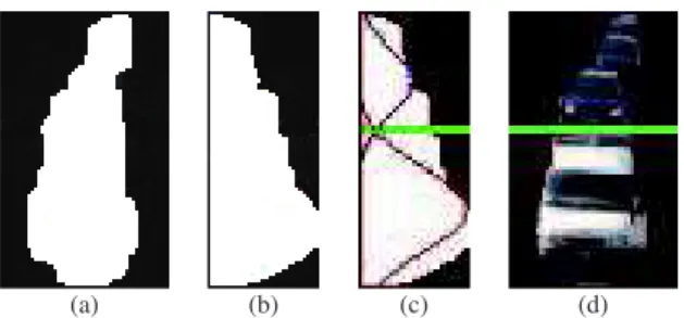
2) Blob splitting: We propose to consider the evolution of the blob width along the axis of the road. In our case, the camera is facing the road and the projection of the road axis can be considered as approximately vertical. The blob splitting procedure analyzes the width of the blob on each row of the smallest bounding box of the blob. Figure 3 (a) illustrates the variation of the blob width along the vertical axis showing, on the left side, the binary image of a blob and, on the right side, the width image where the white pixels belonging to the blob have been grouped at the beginning of each row. So the position of the rightmost white pixel represents the width of the blob. As we do not know the number of vehicles in the blob, we begin to separate it into two new blobs. Then, their solidities are calculated and they are recursively segmented, if necessary.

(a) (b) (c) (d)

Fig. 3. Detected blob (a), variation of the blob width along the vertical axis (b) and blob splitting (c-d).

For a blob of height H, all the widths are represented by a vector containing the marginal sums (here, the number of white pixels) along the rows of the binary image of the blob. Optimally separate the blob comes down to split this width vector into two classes. We use the Minimum Error Thresholding (MinError) algorithm proposed by Kittler et al. in [16]. Considering the vector of the width values of the blob as a mixture of two Gaussian distributions, this algorithm calculates the threshold that minimizes the classification error. The returned value is the row splitting the blob into two parts. From detected blobs, in white in Fig. 3 (a), we obtain the splitting results shown in Fig. 3 (c-d). The two Gaussian curves minimizing the classification error are displayed in red and blue. The corresponding thresholds are represented by green lines.

Occasionally, the iterative MinError algorithm does not converge or converge to a value out of the[0; H − 1] interval. When this occurs, only one Gaussian function is appropriate to approximate the blob widths and the blob is not split. It could happen in two cases: it is possible that the occlusion between two vehicles is so strong that the resulting blob might be convex; a vehicle can also be badly segmented and fail the solidity test.

D. Tracking of the blobs and counting valid trajectories

After the previous modules of motion detection, shadow removal and occlusion management, all blobs do not match necessarily with a single vehicle. Therefore, some artifacts can remain or several blobs can correspond to the same vehicle. A way to overcome this, is to consider trajectories. This is what tracking does. It allows counting a vehicle only once. Kalman filter is very well adapted to the kinds of motion in our sequences (rectilinear and smooth).

First of all, we define a counting zone delimited by two virtual lines. A compromise has to be chosen on its size. This zone has to be large enough to avoid too many false positives and small enough to count every vehicle whatever its size (two-wheelers, small cars...). In our case, we take into account vehicles going on a one-way direction. So, we define a single entry line which is the upper line and a single exit line which is the lower line.

A vehicle is counted if it crosses the counting zone, i.e. if its trajectory begins before the entry line and continues after the exit line.

Then, vehicles are classified into three categories: light vehicles (LV), heavy vehicles (HV) and two-wheelers (TW). The classification is made according to their width compared to that of the road at the exit line level. As in our case we are facing the road, the width is a good discriminating indicator. For some vehicles, like two-wheelers, the tracking begins later because of detection problems. In order to take into account these kind of vehicles, we add a second counting zone which overlaps the first one and reinforces the counting procedure.

IV. RESULTS A. Shadow removal results

The shadow removal module has been evaluated on the Highway I video from the ATON project data-sets [17] with the consent of the UCSD Computer Vision and Robotics Research Laboratory in the Electrical and Computer Engi-neering Department at U.C. San Diego. ATON Highway I is a very interesting video sequence for shadow elimination. It contains many vehicles coming up in front of the camera. There are large shadows from moving vehicles and from the background. This video had been used in some articles for shadow removal [14], [18].

In order to perform a quantitative evaluation of our method and to compare it to a similar method, we have set up a ground truth composed of 64 frames in which we have manually segmented in average 3 vehicles with shadows. So, the total number of vehicles segmented is around 200. The ATON Highway I video was used for that purpose. The performance of the proposed algorithms on shadow elimination is evaluated thanks to recall = number of detected true shadow pixels / number of true shadow pixels, and precision = number of detected true shadow pixels / number of detected shadow

pixels. The numerous shadows carried by the vehicles present several configurations: vehicles far from the sensor so with small shadow areas, vehicles in the central part of the scene and finally vehicles close to the sensor. Many difficulties appear on this set-up. There are single vehicles but also on a same image, few vehicles merged by shadow.

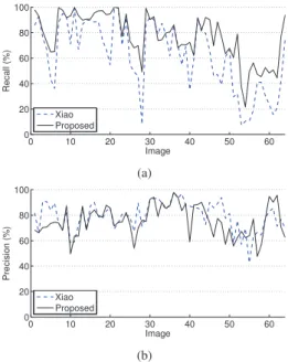
Figure 4 shows the comparison of our method with Xiao’s one. In the first case, where vehicles are isolated, for both methods, results are very similar in most of the time, but our method performs much better in the second case, where several vehicles are present in the scene. On average, from the 64 frames processed, our recall indicator is better than the one of Xiao (77% vs 62%). The precision scores are similar for the two methods. 0 10 20 30 40 50 60 0 20 40 60 80 100 Image Recall (%) Xiao Proposed (a) 0 10 20 30 40 50 60 0 20 40 60 80 100 Image Precision (%) Xiao Proposed (b)

Fig. 4. Recall (a) and precision (b) comparison between our method (in black) and Xiao’s (in dash line) on the 64 images set-up.

Figure 5 shows the comparison between the two methods only for two images extracted from the ATON Highway I video. For the first one, we got a recall rate of 77.36% vs 42.13% for Xiao’s method. For the second one, we obtained 94.15%, whilst Xiao’s method achieves below 70%, 66.95% of recall rate.

B. Vehicle counting

The evaluation work was divided into two stages. During the first stage, we acquired three different data-sets on the same site. This site is also equipped with inductive loops [http://www.transport-intelligent.net/] which are convenient for comparison purposes. The first data-set (named Cloudy) was shot during a cloudy weather, so with cloudy illumination and without shadows. The second one (Sunny) was shot during a very sunny day and with severe shadows. The third one (Transitions) was shot in presence of sparse clouds leading to sudden illumination changes. The three data-sets are approxi-mately 20 minutes long and contain between 1300 and 1500

(a) (b)

Fig. 5. Shadow removal comparison: results from 2 images with shadows: Raw images with vehicle shadows manually segmented on the first row. Vehicle shadows automatically segmented with Xiao method on the second row. Vehicle shadows automatically segmented with our shadow removal module and from our moving region detection result on the last row.

vehicles each, according to the ground truth.

During the second stage, a longer data-set was shot in another site and contains many difficulties due to shadows. It contains 3111 vehicles and is a 37 minutes long video. Casted shadows from vehicles are more spread and stretched due to the sun position.

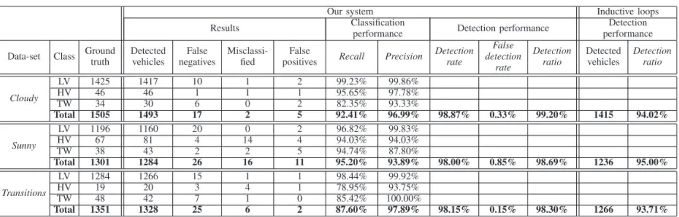
Table 1 shows the vehicle counting and classification results. The ground truth has been obtained manually. For each vehicle class, from the results automatically computed by our system, the number of false negatives (undetected vehicles), false posi-tives (mistakenly counted vehicles) and misclassified (assigned to a wrong class) vehicles, are calculated. The system is evaluated according to:

• classification performance using recall = true positives / ground truth, and precision= true positives / (detected vehicles - misclassified); “Total recall” and “total preci-sion” are the averages of the values obtained with the three vehicle categories;

• detection performance using detection rate = 1 - false negatives / ground truth, false detection rate = false positives / ground truth, and detection ratio = detected vehicles / ground truth.

The results obtained by inductive loops are evaluated using their detection ratio. Based on the detection ratio, vehicle detection results of the video-based system are better than those obtained with the ILD system whatever the data-set considered: 99.2% against 94.02% for Cloudy, 98.69% against 95% for Sunny and 98.3% against 93.71% for Transitions. The detection rate of our system is always greater than 98% and the false positive rate is equal to 0.85% in the worst case. The detection results of two-wheeled vehicles are less good than those of light vehicles. The number of false negatives can be explained by several factors. Their small size, their high

Table 1.Results of the proposed video-based vehicle counting system.

Our system Inductive loops

Results Classification_performance Detection performance _performanceDetection

Data-set Class Ground_truth Detected_{vehicles negatives}False Misclassi-_{fied positives}False Recall Precision Detection_rate False detection rate Detection ratio Detected vehicles Detection ratio Cloudy LV 1425 1417 10 1 2 99.23% 99.86% HV 46 46 1 1 1 95.65% 97.78% TW 34 30 6 0 2 82.35% 93.33% Total 1505 1493 17 2 5 92.41% 96.99% 98.87% 0.33% 99.20% 1415 94.02% Sunny LV 1196 1160 20 0 2 96.82% 99.83% HV 67 81 4 14 4 94.03% 94.03% TW 38 43 2 2 5 94.74% 87.80% Total 1301 1284 26 16 11 95.20% 93.89% 98.00% 0.85% 98.69% 1236 95.00% Transitions LV 1284 1266 15 1 1 98.44% 99.92% HV 19 20 3 4 1 78.95% 93.75% TW 48 42 7 1 0 85.42% 100.00% Total 1351 1328 25 6 2 87.60% 97.89% 98.15% 0.15% 98.30% 1266 93.71%

speed and their non rectilinear trajectories make them difficult to track with the Kalman filter. Moreover, the shadow removal process needs a minimum number of interior edges, which is rarely the case with two-wheelers. It can also be noted that the number of two-wheelers being low, the results have to be interpreted carefully. It is also the case for heavy vehicles in the Transitions data-set. The promising results on the first three data-sets are confirmed by the counting results for the fourth data-set used in the second stage of our experiments. In spite of difficulties induced by road marking and shadows due to road panels, moving tree branches and vehicles, the detection ratio remains very satisfactory, 98.33%, with 3059 detected vehicles out of 3111.

For all the data-sets, the best recall and precision are obtained for the light vehicle category, with a mean recall equal to 98.16% and a mean precision of 99.87%. For the other vehicle categories, the number of misclassified vehicles comes from the low number of classes. Intermediate vehicles, like camping cars or vans for example, supposed to be classified into light vehicles could be classified into heavy cars due to their width. It would be interesting to consider more classes of vehicles to reduce errors and to get a better characterisation of the traffic. But taking into account more categories would require a more sophisticated and discriminant classification criterion than the blob width.

V. CONCLUSIONS

In this paper, we have presented a novel computer vision system devised to track and classify vehicles with the aim of an alternative to complement ILD, particularly on highways. The system has been tested with different kinds of illumination changes (cloudy, sunny, transitions between sun and clouds) obtaining better results than those of ILD. The system can handle casted shadows without the need of any hardware other than cameras and a common computer. Another particular strength of the method proposed is its ability to deal with severe occlusions between vehicles. Multicore programming (with an Intel Core i5 2.67 GHz) allows us to achieve real-time performances (20 frames/s) only with software programming.

REFERENCES

[1] S. Greenhill, S. Venkatesh and G. A. W. West. Adaptive model for foreground extraction in adverse lighting conditions. In Proc. PRICAI,

volume LNCS 3157, 2004.

[2] K. Kim, T. H. Chalidabhongse, D. Harwood and L. S. Davis. Real-time foreground-background segmentation using codebook model. Real-Time

Imaging, 11(3):172–185, 2005.

[3] C. R. Wren, A. Azarbayejani, T. Darrell and A. P. Pentland. Pfinder: real-time tracking f the human body. IEEE Trans. on Pattern Analysis

and Machine Intelligence, 19(7):780–785, 1997.

[4] C. Stauffer and W. E. L. Grimson. Adaptive background mixture models for real-time racking. In Proc. IEEE CVPR, 1999.

[5] J. Rittscher, J. Kato, S. Joga and A. Blake. A probabilistic background model for tracking. In Proc. ECCV, 2000.

[6] L. Unzueta, M. Nieto, A. Cort´es, J. Barandiar´an, O. Otaegui and P. S´anchez. Adaptive multicue background subtraction for robust vehicle counting and classification. IEEE Trans. on Intelligent Transportation

Systems, 13(2):527–540, 2012.

[7] D. Grest, J.-M. Frahm and R. Koch. A color similarity measure for robust shadow removal in real time. In Proc. VMV, 2003.

[8] A. J. Joshi, S. Atev, O. Masoud and N. Papanikolopoulos. Moving shadow detection with low- and mid-level reasoning. In Proc. IEEE

ICRA, 2007.

[9] R. Avery, G. Zhang, Y. Wang and N. Nihan. Investigation into shadow removal from traffic images. Transportation Research Record, 2000:70– 77, 2007.

[10] X. F. Song and R. Nevatia. Detection and tracking of moving vehicles in crowded scenes. In Proc. IEEE WMVC, 2007.

[11] I. Huerta, M. Holte, T. Moeslund and J. Gonz´alez. Detection and removal of chromatic moving shadows in surveillance scenarios. In Proc. IEEE

ICCV, 2009.

[12] B. Coifman, D. Beymer, P. McLauchlan and J. Malik. A real-time computer vision system for vehicle tracking and tracking surveillance.

Transportation Research Part C, 6(4):271–288,1998.

[13] C. C. C. Pang, W. W. L. Lam, and N. H. C. Yung. A method for vehicle count in the presence of multiple-vehicle occlusions in traffic images.

IEEE Trans. on Intelligent Transportations Systems, 8(3):441–459, 2007. [14] M. Xiao, C.-Z. Han, L. Zhang. Moving shadow detection and removal for traffic sequences. Int. Journal of Automation and Computing, 4(1):38–46, 2007.

[15] G. Jun, J. K. Aggarwal and M. Gokmen. Tracking and segmentation of highway vehicles in cluttered and crowded scenes. In Proc. IEEE

Workshop Appl. Comput. Vis., 2008.

[16] J. Kittler and J. Illingworth. Minimum error thresholding. Pattern Recognition, 19(1):41–47, 1986.

[17] Shadow detection and correction research area of the autonomous agents for on-scene networked incident management (ATON) project. http://cvrr.ucsd.edu/aton/shadow/

[18] A. Prati, I. Mikic, M. M. Trivedi and R. Cucchiara. Detecting moving shadows: Algorithms and evaluation. IEEE Trans. on Pattern Analysis