Convergent scheduling : a flexible and extensible scheduling framework for clustered VLIW architectures

Convergent Scheduling: A Flexible and Extensible

Scheduling Framework for Clustered VLIW

Architectures

by

Diego Puppin

B.S., Universita di Pisa, Italy (2000)

M.S., Scuola Normale Superiore di Pisa, Italy (2000)

Submitted to the Department of Electrical Engineering and Computer

Science

in partial fulfillment of the requirements for the degree of

Master of Science in Electrical Engineering and Computer Science

at the

MASSACHUSETTS INSTITUTE OF TECHNOLOGY

December 2002

@

Massachusetts Institute of Technology 2002.

A uthor ...

Department of Electrical

C ertified by ...

BARKER

MAY 1 2 2003

LIBRARIES

All rights reserved.

Enggring*nd

Pter Science

... ... . . . . . .

Saman P. Amjasinghe

Associate Professor

Thesis Supe visor

Accepted by ...

Athur

C. Smith

Chairman, Department Committee on Graduate Students

Convergent Scheduling: A Flexible and Extensible

Scheduling Framework for Clustered VLIW Architectures

by

Diego Puppin

Submitted to the Department of Electrical Engineering and Computer Science on December 15, 2002, in partial fulfillment of the

requirements for the degree of

Master of Science in Electrical Engineering and Computer Science

Abstract

Convergent scheduling is a general instruction scheduling framework that simplifies and facilitates the application of a multitude of arbitrary constraints and scheduling heuristics required to schedule instructions for modern complex processors. A conver-gent scheduler is composed of independent phases, each implementing a heuristic that addresses a particular problem or constraint. The phases share a simple, common in-terface that allows to inquire and modify spatial and temporal preference for each instruction. With each heuristic independently applying its scheduling constraint in succession, the final result is a well formed instruction schedule that is able to satisfy most of the constraints.

We have implemented a set of different passes that addresses scheduling con-straints such as partitioning, load balancing, communication bandwidth, and register pressure. By applying and hand-tuning these heuristics we are able to obtain an average increase in speedup on a 4-cluster clustered VLIW architecture of 28% when compared to Desoli's PCC algorithm [Des98], 14% when compared to UAS [OBC98], and a speedup of 21% over the existing space-time scheduler of the Raw proces-sor [LBF+98].

Because phases can be applied multiple times and in any order, a convergent sched-uler is presented with a vast number of legal phase orderings. We use machine-learning techniques to automatically search for good phase orderings, for three different VLIW architectures. The architecture-specific phase orderings yield speedups ranging from 12% to 95% over the baseline order. Furthermore, cross validation studies that we perform in this work show that our automatically generated orderings perform well beyond the benchmarks on which they were 'trained': benchmarks that were not in the training set are within 6% of the performance they would obtain had they been

in the training set.

Thesis Supervisor: Saman P. Amarasinghe Title: Associate Professor

Acknowledgments

This thesis expands and continues the work described in the paper Convergent Schedul-ing, presented at MICRO-35, Istanbul, November 2002.

I would like to thank the people whose help was important in the completion of this work. First, my advisor Saman Amarasinghe for his support and guidance during these two years. Then, David Maze, Sam Larsen, Michael Gordon and Mark Stephenson for the good group effort in developing the Chorus infrastructure. In particular, I would like to thank Mark for developing the initial genetic programming infrastructure, which was adapted for this work, and for his support to our paper on genetic programming.

I want to acknowledge the contribution given by Shane Swenson, with the initial

work on soft scheduling, and Walter Lee, for his help with Raw compiler and for finalizing the Istanbul paper.

I would like to sincerely thank all the friends that made these two years a wonderful

experience. This space is too small to remember all of them.

This work is dedicated to my family and to Silvia. Without their support and love I could not have made it.

Contents

3.3.2 Placement and Critical Path . . . . 30

3.3.3 Communication and Load Balancing . . . . 33

3.3.4 Register allocation . . . . 35 3.3.5 Miscellaneous . . . . 36 3.4 Collection of Metrics . . . . 37 3.4.1 Graph size . . . . 37 3.4.2 Unplaced . . . . 37 3.4.3 C P L . . . . 37 3.4.4 Imbalance . . . . 38 3.4.5 Number of CPs . . . . 38 3.5 Boolean tests . . . . 39

4 Adapting Convergent Scheduling by means of Genetic Programming 41 4.1 H arness . . . . 43

4.2 Grammar . . . .

5 Compiler Infrastructure

5.1 Chorus Infrastructure . . . .

5.1.1 Partial Component Clustering

5.1.2 Unified Assign-and-Schedule .

5.2 RAW architecture . . . .

5.3 Preplacement Analysis . . . .

(PCC)

6 Results: Comparison with State-of-the-art 6.1 Convergent schedulers . . . .

6.2 Benchm arks . . . .

6.3 Performance comparisons . . . . 6.4 Scheduling convergence . . . .

6.5 Compile-time scalability . . . .

7 Results: Adapting to Different Architectures 7.1 GP Parameters . . . . 7.2 Tested Architectures . . . . 7.2.1 Baseline (4cl) . . . .

7.2.2 Limited bus (4cl-comm) . . . .

7.2.3 Limited bus (2cl-comm) . . . . 7.2.4 Limited Registers (4cl-regs) . . . .

7.3 R esults . . . .

7.3.1 Baseline (4cl) . . . .

7.3.2 Limited Bus (4cl-comm) . . . .

7.3.3 Limited bus (2cl-comm) . . . .

7.3.4 Limited Registers (4cl-regs) . . . .

7.4 Leave-one-out Cross Validation . . . .

7.5 Summary of Results . . . . 8 Related work algorithm implementation 44 47 47 48 50 51 53 Scheduling Techniques 55 . . . . 5 5 . . . . 5 6 . . . . 5 6 . . . . 5 8 . . . . 6 0 63 63 64 64 65 65 65 65 66 66 67 68 68 71 73

List of Figures

1-1 Tradeoff between scheduling and register pressure . . . . 16

1-2 Tradeoff between parallelism and locality . . . . 16

1-3 Two examples of data dependence graphs . . . . 17

1-4 The convergent schedule infrastructure. . . . . 19

2-1 Example of convergence . . . . 23

4-1 Flow of genetic programming. . . . . 42

4-2 Sequence of passes coded as an s-expression . . . . 45

5-1 Chorus VLIW Scheduler . . . . 49

5-2 UAS algorithm . . . . 51

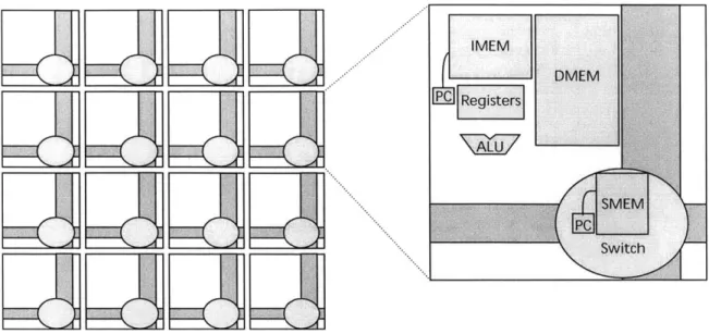
5-3 The Raw m achine. . . . . 52

6-1 Performance comparisons between Rawcc and Convergent scheduling on a 16-tile Raw machine. . . . . 58

6-2 Performance comparisons between PCC, UAS, and Convergent schedul-ing... ... 59

6-3 Convergence of spatial assignments on Raw. . . . . 59

6-4 Convergence of spatial assignments on Chorus. . . . . 60

6-5 Comparison of compile-time vs input size for algorithms on Chorus. 61 7-1 Speedup on 4cl-comm . . . . 67

7-2 Fitness of the best individual, during evolution on 4cl-comm. . . . . . 68

7-4 Speedup on 4cl-regs. . . . . 70 9-1 A compiler with dynamic policy for choosing passes . . . . 79

List of Tables

3.1 Pseudo-code for the driver of convergent scheduling . . . . 28

3.2 The algorithm LevelDistribute. . . . . 35

4.1 Grammar for genome s-expressions. . . . . 44

6.1 Sequence of heuristics used by the convergent scheduler for the Raw machine and clustered VLIW . . . . 56

6.2 Characteristics of tested benchmarks . . . . 57

6.3 Speedup on Raw . . . . 57

7.1 Parameters of the evolutionary framework . . . . 64

7.2 Results of cross validation. . . . . 71

Chapter 1

Introduction

Instruction scheduling on microprocessors is becoming a more and more difficult prob-lem. In almost all practical instances, it is NP complete, and it often faces multiple contradictory constraints. For superscalars and VLIWs, the two primary issues are parallelism and register pressure. Code sequences that expose much instruction level parallelism (ILP) also have longer live ranges and higher register pressure. To gen-erate good schedules, the instruction scheduler must somehow exploit as much ILP as possible without leading to a large number of register spills. Figure 1-1 shows an example from [MPSR95] of such tradeoff.

On spatial architectures, instruction scheduling is even more complicated. Exam-ples of spatial architectures include clustered VLIWs, Raw [WTS+97], Trips [NSBKO1], and ILDPs [KS02]. Spatial architectures are architectures that distribute their com-puting resources and the register file. Communication between distant resources can incur one or more cycles of delays. On these architectures, the instruction sched-uler has to partition instructions across the computing resources. Thus, instruction scheduling becomes both a spatial problem and a temporal problem.

To make partitioning decisions, the scheduler has to understand the proper trade-off between parallelism and locality. Figure 1-2 shows an example of this tradetrade-off. Spatial scheduling by itself is already a more difficult problem than temporal schedul-ing, because a small spatial mistake is generally more costly than a small temporal mistake. If a critical instruction is scheduled one cycle later desired, only one cycle is

5 6 4 AF

(b)

(d

Figure 1-1: An example of tradeoff between aggressive scheduling and register pres-sure. Rectangles are instructions; edges between rectangles represent data depen-dences, with circles on them representing delays due to instruction latency. The circles on the left represent the time axis. Consider a single-issue machine with two registers and two-cycle loads. Figure (a) shows an aggressive schedule that attempts to overlap the load latencies. After cycle three, there are three live ranges, so one value must be spilled. The spilling leads to the code sequence in (b), which takes nine cycles. If instead the scheduler tries to minimize register pressure, we end up with schedule (c), which still takes eight cycles. The optimal schedule, in (d), takes only seven cycles, and it exhibits a careful tradeoff between aggressive scheduling and register pressure minimization.

2 MT 3 4 (a) 7 I 3 MUL 2 3 4ADD 4 T (b)() " 1 5 MUL 2 3 6 ADD (c) I I

Figure 1-2: An example of tradeoff between parallelism and locality on spatial ar-chitectures. Each node color represents a different cluster. Consider an architecture with three clusters, each with one functional unit and three registers, where commu-nication takes one cycle of latency due to the receive instruction. In (a), conservative partitioning that maximizes locality and minimizes communication leads to an eight-cycle schedule. In (b), aggressive partitioning has high communication requirements and leads to an eight-cycle schedule. The optimal schedule, in (c), takes only seven cycles: it is a careful tradeoff between locality and parallelism.

(a) (b)

7~ It

(a) (b)

Figure 1-3: Two examples of data dependence graphs. (a) is a typical example from a non-numeric program, (b) is common in unrolled numerical loops

lost. But if a critical instruction is scheduled one unit of distance farther away than desired, cycles can be lost from unnecessary communication delays, additional com-munication resource contention, and increase in register pressure. In addition, some instructions on spatial architectures may have specific spatial requirements. For ex-ample, these requirements may arise from the need to access specific spatial resources, such as a specific memory bank [BLAA99]. A good scheduler must be sensitive to these constraints in order to generate a good schedule.

A scheduler also faces difficulties because different heuristics work well for different

types of graphs. Figure 1-3 depicts representative data dependence graphs from two ends of a spectrum. In the graphs, nodes represent instructions and edges represent data dependences between instructions. Graph (a) is typical of graphs seen in non-numeric programs, while graph (b) is representative of graphs coming from applying loop unrolling to numeric programs. Consider the problem of scheduling these graphs

onto a spatial architecture. Long, narrow graphs are dominated by a few critical paths. For these graphs, critical-path based heuristics are likely to work well. Fat, parallel graphs have coarse grained parallelism available and many critical paths. For these graphs it is more important to minimize communication and exploit the coarse-grain parallelism. To perform well for arbitrary graphs, a scheduler may require multiple heuristics in its arsenal.

Traditional scheduling frameworks handle conflicting constraints and heuristics in an ad hoc manner. One approach is to direct all efforts toward the most serious problem. For example, modern RISC superscalars can issue up to four instructions and have tens of registers. Furthermore, most integer programs tend to have little ILP. Therefore, many RISC schedulers focus on finding ILP and ignore register pres-sure altogether. Another approach is to address the constraints one at a time in a sequence of phases. This approach, however, introduces phase ordering problems, as decisions made by the early phases are based on partial information and can ad-versely affect the quality of decisions made by subsequent phases. A third approach is to attempt to address all the problems together. For example, there have been reasonable attempts to perform instruction scheduling and register allocation at the same time

[MPSR95].

Also, commercial processors can share the same Instruction-Set Architecture, but with very different internal organizations. The cost of targeting with effectiveness the new architecture grows with the faster turn-over of processor generations. A system to address this, in an automatic manner, is strongly needed.

This thesis presents convergent scheduling, a general scheduling framework that makes it easy to specify arbitrary constraints and scheduling heuristics. Figure 1-4 illustrates this framework. A convergent scheduler is composed of independent phases. Each phase implements a heuristic that addresses a particular problem such as ILP or register pressure. Multiple heuristics may address the same problem.

All phases in the convergent scheduler share a common interface. The input and

instruc-COLLECTION OF HEURISTICS Preplaced Insirs [ntcai Pa

INPUT Neighbors Ldbanc

OUTPUT

Dependence Graph

Preplaced _{Convergent Time-space}

I"str'"ctio _Scheduler

Schedule Info

Machine Model and Other Constraint!

Figure 1-4: The convergent schedule infrastructure.

tions. A phase operates by modifying these data. As the scheduler applies the phases in succession, the preference distribution will converge to a final schedule that incor-porates the preferences of all the constraints and heuristics. Logically, preferences are specified as a three-input function that maps an instruction, space, and time three-tuple to a weight.

In our first work with convergent scheduling, we tediously hand-tuned the phase order. While the sequence works well for the processors we initially explored, it does not generally apply to new architectural configurations. As we add new phases to our scheduler to address next generation architectural features, hand-tuning the sequence of passes becomes even harder.

To complicate matters, architectures evolve quickly. Even though a processor family may share the same programming interface (ISA), the internal organization of the processors can differ dramatically (e.g., number of registers, functional units, etc.). It is the compiler's task to address the architectural features efficiently, by determining a schedule that matches the constraints. Time-to-market pressures make it extremely difficult to effectively target new architectures.

This thesis uses machine learning techniques to automatically find good phase orderings for a convergent scheduler. We show how our system can automatically discover architecture-specific phase orders. Because different parallel architectures have unique scheduling needs, the speedups our system is able to obtain by creating architecture-specific phase orderings is impressive. Equally impressive is the ease with

which it finds effective sequences.

Using a modestly sized cluster of workstations, our system is able to quickly find good convergent scheduling sequences. In less than two days, it discovers sequences that produce speedup ranging from 12% to 95% over previous work. Furthermore,

by varying architectural parameters and rerunning the experiment, we show that

different architectures indeed have special compilation requirements. The learning algorithm catered a sequence of passes to each of the three architectures on which we tested it.

The main contributions of this thesis are:

* a novel approach to address the combined problems of partitioning, scheduling, and register pressure,

e the formulation of a set of powerful heuristics to address very general constraints

and some architecture-specific issues,

e a demonstration of the effectiveness of convergent scheduling, which is able to

surpass more complex combined solutions,

* the use of machine learning to adapt convergent scheduling to a new architec-ture.

The rest of this thesis is organized as follows. Chapter 2 introduces convergent scheduling and uses an example to illustrates how it works. Chapter 3 gives more

detail about infrastructure and implementation. Chapter 4 discusses how the system can be adapted to different architectures by means of genetic programming. Chapter 5 illustrate our compiler infrastructure and the schedulers we used for our experimental comparisons. Chapter 6 presents results for a clustered VLIW architecture and for the Raw processor. Chapter 7 describes the framework and the results we reached when we adapted our system to different VLIW architectures. Chapter 8 provides related work. Chapter 9 highlights future work and concludes.

Chapter 2

Convergent scheduling

In this chapter, we introduce convergent scheduling by giving an example of its work

on a basic block from fpppp. With this, we show the peculiar features of the system and how it avoids some of the problems typical of more traditional compilers.

In the convergent scheduling framework, passes communicate their choices as changes in the relative preferences of different schedules. A pass works by manip-ulating the weight for a specific instruction to be scheduled at a specific cycle, in a specific cluster.1 _{At the end of the algorithm, every instruction will be scheduled in}

the space-time slot with the heighest weight, which we call the preferred slot.

Different heuristics work to improve the schedule in different ways. The critical

path (CP) strengthening heuristic, for example, expresses a preference to keep all

the instructions in the CP together in the same cluster, by determining the best cluster for this, and by increasing the preference (weights) for those instructions to be scheduled there. The communication minimization heuristic tries to keep dependent instructions (neighbors) in the same cluster, by computing for every instruction where most of its neighbors are, and then by increasing the preference for that cluster. The

preplacement heuristic considers the congruence information, as defined in [LA02], to

exploit the memory parallelism while preserving locality. If the memory is banked and every bank is local to a cluster, this heuristic increases the preference to keep memory

'In the rest of this thesis, we will use interchageably the terms phases and passes, tile and cluster, and cycle and time slot.

instructions in the cluster where most of the dynamic instances of the instruction are local. The load balance heuristic reduces the preferences on the most loaded cluster, and increases them on the least loaded one. Other passes will be introduced in section 3.3.

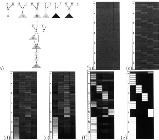
Figure 2-1 shows how convergent scheduling operates on a small code sequence from fpppp. In this simple example, we will focus only on the heuristics that address space allocation. Figure 2-1(a) shows the data dependence graph of the code se-quence. Each node is an instruction, and each edge represents a dependence between instructions. Triangular nodes represent preplaced instructions. For simplicity, the example only illustrates space scheduling, not the combined space and time schedul-ing. Each of the figures 2-1(b-g) is a cluster preference map. A row represents an instruction. The row numbers corresponds to the instruction numbers in (a). A col-umn represents a cluster. The color of each entry represents the level of preference an instruction has for that cluster. The lighter the color, the stronger the preference. Initially, the weights are evenly distributed, as shown in (b). We apply the noise

introduction heuristic to break symmetry, resulting in (c). This heuristic helps

in-crease parallelism by distributing instructions to different clusters. Then, we run

critical path (CP) strengthening, which increases the weight of the instructions in

the CP (i.e. instructions 23, 25, 26, etc.) in the first cluster (d). Then we run the

communication minimization and the load balance heuristics, resulting in (e). These

heuristics lead to several changes: the first few instructions are pushed out of the first cluster, and groups of instructions start to assemble in specific clusters (e.g. instructions 19, 20, 21, and 22 in the third cluster).

Next, we run a preplace biasing pass that utilizes information about preplaced nodes. The result is shown in (f). This pass causes a lot of disturbances: preplaced instructions strongly attract their neighbors to the same cluster. Observe how the group 19-22 is attracted to the last cluster. Finally we run communication

minimiza-tion another time. The final schedule is shown in (g).

The schedule is very effective because it reaches a good trade-off over conflict-ing opportunities: parallelism is exploited, but keepconflict-ing in consideration the memory

19 20 21 22 (a) (d)L 16 15 24 23 2 1 17 25 3 T -1 28 6 31 32 (e). 8 7 12 11 0 9 13

(f)LE

Figure 2-1: Convergence scheduling operates on a code sequence in from fpppp. Rows represent the different instructions i in the block, columns are the (four) clusters c in the architecture. Every slot (i, c) represents the weight of i to be scheduled on cluster

c. The brighter the color, the higher the weight. The dependence graph relative to the

block is shown. Triangular nodes are preplaced, with different shades corresponding to different clusters. Rows are numbered according to the node numbers in the graph. layout and instruction preplacement; critical path is kept together so to minimize delays due to communication; independent subcomponents of the graph are moved to unused tiles.

Convergent scheduling has the following features:

1. Its scheduling decisions are made cooperatively rather than exclusively.

2. The interface allows a phase to express confidence about its decisions. A phase needs not make a poor and unrecoverable decision just because it has to make a decision. On the other side, any pass can strongly affect the final choice if needed.

3. Convergent scheduling can naturally recover from a temporary wrong decision by one phase. In the example, when we apply a randomizer to (b), many nodes

are initially moved away from the first cluster. Subsequently, however, nodes with strong ties to cluster one, such as nodes 1-6, are eventually move back, while nodes without strong ties, such as node 0, remain away.

4. Most compilers allow only very limited exchange of information among passes. In contrast, the weight-based interface to convergent scheduling is very expres-sive.

5. The framework allows a heuristic to be applied multiple times, either

inde-pendently or as part of an iterative process. This feature is useful to provide feedback between phases and to avoid phase ordering problems.

6. The simple interface (preference maps) between passes makes it easy for the

compiler writer to handle new constraints or design new heuristics. Phases for different heuristics are written independently, and the expressive, common in-terface reduces design complexity. This offers an easy way to retarget a compiler and to address peculiarities of the underlying architecture. If, for example, an architecture is able to exploit auto-increment on memory-access with a specific instruction, one pass could try to keep together memory-accesses and incre-ments, so that the scheduler will find them together and will be able to exploit the advanced instruction.

7. The very clean design allows to easily re-order, add or remove passes from the

compiler. This gave us the opportunity to design a system that evolves the sequence of passes in order to adapt to the underlying architecture.

Chapter 3

Implementation

This chapter describes in detail our implementation of convergent scheduling: the way we implemented preferences; the driver infrastructure; our heuristics; the set of metrics we used in our adaption experiments, and how we combined them into boolean tests.

3.1

Preferences

Convergent scheduling operates on individual scheduling units, which may be basic blocks, traces, superblocks, or hyperblocks. It stores preferences in a three dimen-sional matrix Wi, where i spans over all instructions in the scheduling unit, c spans over the clusters in the architecture, and t spans over time. We allocate as many cycles as the critical-path length (CPL), with the goal of finding an optimal schedule that fits the CPL. Even when this is not possible, our framework allows us to return rich information that will allow to build an optimal schedule in this case too. This is due to the fact that we compute a preference map that is much richer than a simple time schedule for the instructions. For example, our system can in fact verify the presence of phases in the schedule, which can be highlighted and brought to the at-tention of the list scheduler: the system can identify feasible and unfeasible time-slots for each instruction in the final schedule, more than just giving a time schedule.

depen-dence graph and the weight matrix to determine the characteristics of the preferred schedule so far. Then, it expresses its preferences by manipulating the preference map. Passes are not required to perform changes that affect the preferred schedule.

If they are indifferent to one or more choices, they can avoid any changes, or change

weights only slightly. It can be the case that following passes will pick up the hint to change the preferred schedule.

If i spans over instructions, t over time-slots, c over clusters, we have:

Vi, c, t : 0 < Wj,,,c < 1

Vi: Wit,c = 1

Ct

We define:1

preferred time(i) dearg max t W₂,t,c

C

preferred cluster(i) arg max c: Wit,c}

def C Wi,t,c-;

runnerup _cluster W) - arg max

c

#

confidence(i) = Et Wi,t,preferred _cluster(i) E Wi,,runnerup_cluster(i)

Preferred values are those that maximize the sum of the preferences over time and clusters. The preferred schedule is the one obtained by assigning every instruction to its preferred space-time slot. The runner-up cluster is the second best. The confidence is given by the ratio of the preference for the preferred and the runner-up cluster.

Some basic operations are available on the weights:

'The function arg max returns the value of the variable that maximizes the expression for a given set of values (while max return the value of the expression). For instance max{0 < x < 2 : 10 - x}

" the weight of a specific instruction to be scheduled in a given space-time slot

can be increased or decreased by a constant, and multiplied or reduced by a factor;

* the system keeps track of the sums over rows and columns, and of their

maxi-mum, so it can quickly, in time 0(1), determine the sum of weights over time

and clusters, and then the preferred space-time slot;

" the preferences can be normalized to guarantee our invariants; the normalization

simply performs:

for each i, t c, Wi,tc <- i'tC Zc't wI/Vt'c

3.2

Configurable Driver

Convergent scheduling works on the SUIF representation of scheduling units (blocks, in the following).2 The chosen sequence of passes is described by a genome, which allows conditional execution of certain passes.3

The convergent scheduler creates a preference matrix for the block, runs the chosen passes, updates the preferences according to each pass, determines a preferred time-space schedule (see table 3.1). This information is then passed to a list scheduler, and then to the register allocator. As explained, convergent scheduling determines the optimal schedule considering the needs of the list scheduler and the register allocator, so the performance of these two parts is predictable.

In chapter 5, we will give more details about how we integrated convergent schedul-ing with our compiler infrastructure.

2

Basic blocks for the Chorus clustered VLIW system, and single-entry single-exit regions, flat-tened with predication, for RAW.

3

For the moment, let just think at the genome as a simple sequence of passes. For more detail, see section 3.4.

function convergentscheduling:

input: CFG describing the scheduling unit, genome describing the sequence of passes

output: instruction partition partition(),

instruction priorities priority() build the empty preference matrix for every pass p in the genome:

apply the pass on the preference matrix update and normalize the matrix for every instruction i:

partition(i) = preferred cluster(i) priority(i) = preferredtime(i)

Table 3.1: Pseudo-code for the driver of convergent scheduling

3.3

Collection of Heuristics

The previous sections introduced the driver and the common data structure used by the heuristics of convergent scheduling. This section introduces the rich collection of heuristics we have implemented so far. Each heuristic attempts to address a single constraint and only communicates with other heuristics via the weight matrix. There are no restrictions on the order or the number of times each heuristic is applied.

3.3.1

Time Heuristics

Initital time assignment (INITTIME)

Instruction in the middle of the dependence graph cannot be scheduled before their predecessors, nor after their successors. So, if CPL is the length of the critical path, l is the length of the longest path from the top of the graph (latency of predecessor chain), and 1, is the longest path to any leaf (latency of successor chain), the instruction can be scheduled only in the time slots between l and CPL - i. If

pass squashes to zero all the weights outside this range.

for each i, (t < lP U t > CPL - ls), c, W,t,c +- 0

When we normalize, the weight for the suitable time-slots will increase suitably. With some effort, this pass can anyway be expressed in a close form that keeps the invariants. This is true also for the other passes listed here. We will give here implementations exploiting normalization instead of close expressions when they are simpler.

Si Z EC'1P<t<CPL-, 8 W ,1,c

WictS if l, < t < CP L - i

for each i, c, t, Wi,C <-

{

0 otherwise

A pass similar to this one can address the fact that some instructions cannot be

scheduled in certain clusters in specific architectures, simply by squashing the weights for the unfeasible clusters.

Dependence enforcement (DEP)

Sometimes, a pass can change weights so that the preferred time of an instruction i

is earlier than that of another instruction

j

(j

this case, to help the convergence, we reduce the weights for i to be scheduled before the preferred time tj of

j

for each i, for each

j

for each c, 0 < t < t3 + latency(j),

Functional units (FUNC)

This pass considers the utilization of the functional units for every time slot. If a time-space slot is overburdened by a large number of instructions, their weights for that slot are reduced. At the moment, this heuristic assumes that there is just one general purpose functional unit available per slot, but this can be easily extended to consider the number and type of functional units in the machine.

load(c, t) - K Wit,c

.oa t 0.9W,,c if load(c,t) > 1

for each

t,

We,, <-{otews

Wit,c otherwise

Emphasize critical path distance (EMPHCP)

This pass attempts to help the convergence of information about time by emphasizing the level of each instruction. Given instruction i, we define level(i) to be its distance from the furthest root. The level of an instruction is a good time approximation because it is when the instruction can be scheduled if a machine has infinite resources.

for each (i, c), Wi,IeveI(i),c - i.2Wi,level(i),c

3.3.2

Placement and Critical Path

Push to first cluster (FIRST)

In the clustered VLIW infrastructure we used, an invariant is that all the data are available in the first cluster at the beginning of every block. For this architecture, we want to give advantage to a schedule that utilizes the first cluster, where data are already available, more than the other clusters, where copies can be needed. In our framework this is easily expressed.

Preplacement (PLACE)

This pass increases the weight for preplaced instructions in their home cluster. In our experiments with clustered architectures, we verified the importance of loop unrolling and of exploiting correctly the local memory. An access to a local memory location is faster and more efficient than an access to remote memory (in another cluster). That is why we want to place a static memory operation in the cluster to which most of its dynamic instances refer. This is called the memory operation's

home cluster. In both Raw and the Chorus clustered VLIW architecture, the home

cluster is determined using congruence analysis [LA02].

for each i, t, c, if i preplaced Wi,,,c Wei,c if c is the home cluster

0 otherwise

Preplacement propagation (PLACEPROP)

This pass propagates preplacement information to all instructions. For each non-preplaced instruction i, we divide its weight on each cluster c by its distance to the closest preplaced instruction in c. Let dist(i, c) be this distance. Then,

for each (i V PREPLACED, t, c),

Wi,t,c - Wj,t,c/dist(i, c)

Critical path strengthening (PATH)

This pass tries to keep all the instructions on a critical path (CP) in the same cluster.

If instructions in the paths have bias (preplacement) for a particular cluster, the path

is moved to that cluster. Otherwise the least loaded cluster is selected. If different portions of the paths have strong bias toward different clusters (e.g. when there are two or more preplaced instructions on the path), the critical path is broken in two or more pieces and kept locally close to the relevant home clusters. Let cc(i) be the chosen cluster for the CP.

for each (i E CP, t, c), W ,t,cc(<) a 3Wjt,cc(j)

Path propagation (PATHPROP)

This pass selects high confidence instructions and propagates their convergent matri-ces along a path. The confidence threshold t is an input parameter. Let Zh be the

selected confident instruction. The following propagates ih along a downward path:

given th

for each i E successor(ih) : confidence(i) < confidence(ih),

for each (c, t), Wi,t,c - .5W,t,c + 0.5Wih,t,c

A similar function that visits predecessors propagates ih along an upward path.

Create clusters (CLUSTER)

PLACE was found to be a very strong and effective heuristics. Nonetheless, if the

program to be compiled does not feature natural preplacement, we try to build clusters of nodes which should stay together, and we distribute them across tiles trying to improve parallelism. This heuristic is rather complex, we will try to give here a high-level overview.

1. identify the candidate clusters, using Desoli's partial_ components algorithm

(see [Des98]), with threshold equal to the size of the graph divided by the number of tiles,

2. for every instruction cluster:

(a) if some instructions are preplaced, skip to the next;

(b) otherwise, assign it to the next cluster (round-robin), by marking its center

3. run a modified PLACE which keeps into account marked instructions as if they

were preplaced.

Heuristically, we consider the center of the cluster as the instruction that was added to the cluster as the N/2-th, if the size of the cluster is N. In the future, we are planning to use the DSC algorithm to build cluster [GY94].

3.3.3

Communication and Load Balancing

This pass reduces communication load by increasing the weight for an instruction to be in the same clusters where most of neighbors (successors and predecessors in the dependence graph) are. This is done by summing the weights of all the neighbors in a specific cluster, and using the sum to skew weights in the correct direction.

for each i, t, C, Witc & Witc - W,t,c

t,nEneighbors of i

We wrote a version of this pass that considers grand-parents and grand-children. We usually run it together with COMM.

Parallelism for successors (SUCC)

This is an example of an architecture-specific pass. In some configurations of our clus-tered VLIW infrastructure, data passed from one cluster to another can be snooped

by other clusters. This way, we can easily implement a broadcast operation. We

ex-ploit this fact by scattering the successors of any instructions to the various clusters if some successor is already placed in a different cluster (a communication is already needed). This is going to improve parallelism and reduce register pressure without requiring more communication.

for each i, if

{successors(i)}

and In, : (preferred cluster(ni)

#

{successors(i)},

r <- randomly chosen cluster

Wit,, - 2 Wi,,r

Load balance(LOAD)

This pass looks for the most loaded cluster, and reduces the weight of instructions to be scheduled there (so increasing the weight for the other slots).

def

max cluster arg max

{c

for each i, t, W,,c

{

1.1Wi,t,c otherwise

Level distribute (LEVEL)

This pass distributes instructions at the same level across clusters. Level distribution has two goals. The primary goal is to distribute parallelism across clusters. The second goal is to minimize potential communication. To this end, the pass tries to distribute instructions that are far apart, while keeping together instructions that are near each other.

To perform the dual goals of instruction distribution without excessive communi-cation, instructions on a level are partitioned into bins. Initially, the bin B, for each cluster c contains instructions whose preferred cluster is c, and whose confidence is greater than a threshold, here equal to 2. The algorithm is described in table 3.2.

The parameter g controls the minimum distance granularity at which we distribute instructions across bins. The distance between an instruction i and a bin B is the minimum distance between i and any instruction in B.

LEVEL can be applied multiple times to different levels. Currently we apply it every four levels on Raw. The four levels correspond approximately to the minimum

LevelDistribute: input int 1, int g

I = Instruction i : level(i) = I

for each c,

I = 1 - Be

19 = {i E I1 : distance(i, find_ closest _bin(i)) > g}

while 1 # q5

B = roundrobinnextbin()

t

closest = arg max{i E Ig : distance(i, B)}

B = B U iclosest

I1 I= -~ iclosest

Update 19 for each c,

for each i C B,

for each t, W,tC +- 10Wic

Table 3.2: The algorithm LevelDistribute.

granularity of parallelism that Raw can profitably exploit given its communication

cost.

3.3.4

Register allocation

Break edges (EDGES)

This pass tries to compute the number of live ranges at a specific time t and cluster c.

We approximate this number with the number of edges the head of which is scheduled before t and the tail after t.This clearly does not take into account the fact that two or more edges could be referring to the same variable, but it is a good approximation

before register allocation.

In the convergent scheduling framework, we have to consider the weight associated to a specific time-space schedule. For every edge, et,c is defined as the product of the sum of the weights for the head to be scheduled before t and for the tail to be scheduled after t. If the total weighted number of edges is large than N the number of registers in the architecture, we reduce the weights on t, with the goal of breaking the edges, i.e. scheduling the head after t or the tail before t.

head(i, T, c) =

Lt

tail(l, T, c) = e>~ W1,,,c

for each c, t,

if (Zedges(ab) head(a, t, c) * tail(b, t, c)) > N

for each i, W,c,t <- 0.8Wi,c,t

Reduce parallelism (SEQUENTIAL)

This pass tries to keep together (time- and space-wise) instructions that follow each other in the original set of instructions and that are dependent from each other. We do so by increasing the weight of the instruction following i to be in the same preferred cluster c., and in the next time slots of the preferred time ti, that is tj + 1.

This is going to minimize the number of temporary values with long life span. This clearly has an effect of performance, because it reduces parallelism, and so it requires careful balancing with other heuristics.

next(i) first dependent instruction following i in the block for each i, Wnext(i),ti,ci +- 1.2Wnext(i),t+1,ci

3.3.5

Miscellaneous

Noise introduction (NOISE)

This pass introduces some noise in the weight distribution, so to break symmetry for subsequent choices. This is important, for instance, in order to have a good allocation of the critical path. After the PATH pass has identified the critical path, the presence of noise will help to perform an unbiased choice of the target cluster. This can defend the system from worst-case scenarios.

Assignment strengthening (BEST)

This pass simply boosts the preference for the preferred slot for every instruction. This is useful as a last pass, but also as a middle pass, in order to strengthen the preferences till the point. If t, and ci are again the preferred time and cluster for i:

for each i, Wit,,c, - 2Wt,,c,

3.4

Collection of Metrics

Along with the passes, we designed a series of metrics, used to measure and determine the current status of the schedule, and the shape of the block being analyzed. Our system is going to exploit this information in order to choose the best passes to run, and the strength used by them: the driver for convergent scheduling can execute one or more passes conditionally, according to the results returned by the metrics.

3.4.1

Graph size

This returns the number of instructions in the block, and can be used to build more complex expressions.

3.4.2

Unplaced

Unplaced returns the number of instructions that are further than a distance of 4

from a preplaced instructions, or that are close (within distance 4) to two (or more) instructions preplaced to different clusters. If unplaced is high, it means that com-munication will be needed to move data across clusters, because instruction will not naturally partition into clusters. In this case, COMM will be needed to minimize the delays due to communication

3.4.3

CPL

3.4.4

Imbalance

Imbalance is a measure of the load-balance in the current schedule: it returns the

maximum difference of load between any two clusters. If a block is particularly imbalanced, the LOAD pass can effectively improve the overall scheduling. Also, a block can be imbalanced because of the presence of the very long critical path that dominates the schedule. In this case, discriminating on the number or the size of critical paths can help take further decisions on the schedule.

def

load(c) Ei & Wi,,,c

imbalance - max{i,j : Iload(i) - load(j)}

3.4.5

Number of CPs

This function returns the number of independent paths the length of which equals the critical path (CP) length. This is used to determine the parallelism present within the analyzed scheduling unit. The presence of multiple critical path can be caused

by unrolling or by intrinsic parallelism in the program. Independent critical path can

effectively be assigned to different cluster with no performance penalty.

determine one critical path CP

numberofCPs = 0 CPL +- length(CP)

mark every i C CP as used

for each r C roots,

find the longest length path P from r if all i c P are not marked as used

numberofCP +=1

mark every i E P as used

3.5

Boolean

tests

These metrics have been combined into simple boolean tests that can be used by the driver to perform choices on the schedule. We are planning to extend our genome syntax to include arithmetic expressions and comparison. In such an infrastructure, this simple boolean tests will not be necessary anymore.

Is imbalanced is true if imbalance is larger than 1/numcluster.

Is fat is true if number of CPs is larger than the number of tiles.

Is within CPL is true if the number of instructions in the block is smaller than the

number of tiles times the CPL.

Is placement bad is true if the number of unplaced instructions is more than half

Chapter 4

Adapting Convergent Scheduling

by means of Genetic Programming

From one generation to the next, architectures in the same processor family may have extremely different internal organizations. The Intel Pentium® family of processors is a case in point. Even though the ISA has remained largely the same, the inter-nal organization of the Pentium 4 is drastically different from that of the baseline Pentium.

To help designers keep up with market pressures, it is necessary to automate as much of the design process as possible. In our initial work with convergent scheduling, we tediously hand-tuned the sequence of passes. While the sequence works well for the processors we explored in our previous work, it does not generally apply to new architectural configurations. Different parallel architectures necessarily emphasize different grains of computation, and thus have unique compilation needs.

We therefore developed a tool to automatically customize our convergent sched-uler to any given architecture. The tool generates a sequence of phases from those described in section 3.3. This chapter describes genetic programming (GP), the machine-learning technique that our tool uses.

Genetic programming (GP) is one of many machine-learning techniques. Like other learning algorithms, GP is based on the idea of evolution: a population of individuals are set to compete against each other in a specific task. The fittest

Compile and run each expression

gens < LIMIT?

No Yes

Probabilistically select expressions

rossover and mutation gens = gens + 1

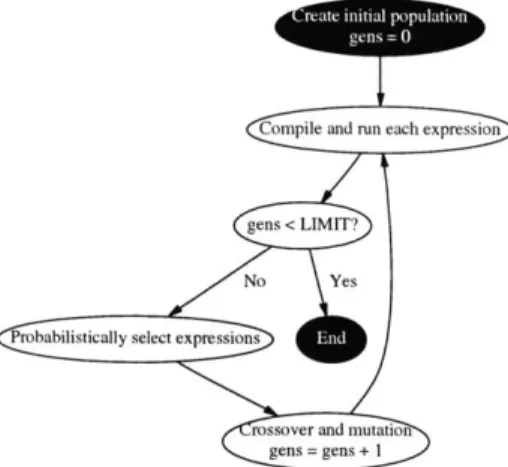
Figure 4-1: Flow of genetic programming. Genetic programming (GP) initially creates a population of expressions. Each expression is then assigned a fitness, which is a measure of how well it satisfies the end goal. In our case, fitness is proportional to the execution time of the compiled application(s). Until some user-defined cap on the number of generations is reached, the algorithm probabilistically chooses the best expressions for mating and continues. To guard against stagnation, some expressions undergo mutation.

ones are able to reproduce and generate off-springs, which will carry on the fight for survival. As in the Darwinian representation of evolutions, the least fit creatures will not replicate their genome, which will disappear from the population. GP models sexual reproduction, by having cross-over of the genomes of the fittest individuals, and allows random mutations to introduce new genomes in the population.

GP has a set of features that makes it particularly fit to our task: it is suited

to explore high-dimensional spaces; it is highly scalable, highly parallel and can run effectively on a distributed computer farm; it presents solution that are readable to humans, compared with other algorithms (e.g. neural networks) where the solution is embedded in a very complex state space.

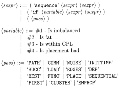
In the general GP framework, individuals are represented as parse trees [Koz92]. They are interpreted as a conditional sequence of passes: a grammar for our expres-sions is in table 4.1.

4.1

Harness

The harness used in our experimentation is adapted from the work of [SAMO02], the structure of which is described in figure 4-1.

The system controls the evolution of a set of expressions challenged with the com-piling of a set of benchmarks. The initial, given seed expression is used to compile and run all benchmarks. The performance (elapsed number of cycles needed to complete the execution) is stored as a reference for each benchmark.

An initial set of individuals is created randomly to populate the world. Each genome is tested against the benchmarks. The fitness is determined by computing the average of the speed-up on single benchmarks, compared with the baseline running time. Individuals with the best performance are considered the fittest. As a secondary criterion, we favors individuals with shorter genomes, as in [Koz92, p. 109]. Shorter sequences offer more insight in the problem under analysis, are easier to read and understand, and lead to a shorter and faster compiling.

The fittest individuals are chosen to mate and reproduce. Sexual reproduction is an important part of GP: sub-expressions from strong individuals are swapped at the moment of reproduction (cross-over). This contributes to add variety to the popula-tion, and to reward strong genomes. Our harness uses a strategy called tournament

selection, to choose the individuals that will reproduce. The tournament randomly

chooses a set of n individuals, and then choose the best of them for reproduction (see [Koz92]).

In our framework, the reproduction by crossover chooses two subtrees from each of the parents, which are swapped to create two off-springs. As in [KH99], our harness uses depth-fair crossover, which gives fair opportunity to all the levels in the tree: a naive approach would choose leaves more often (in a binary tree, 50% of nodes are leaves).

After the off-springs are generated, a subset of them is subject to random muta-tions, which increase further the diversity in the genetic pool. The process iterates till the number of generations reaches a chosen number.

Ksexpr)

('if' (variable) (sexpr) (sexpr)

)

(variable) ::= #1 - Is imbalanced

#2 - Is fat

#3 - Is within CPL #4 - Is placement bad

(pass) 'PATH' 'COMM' 'NOISE' 'INITTIME'

'SUCC' 'LOAD' 'EDGES' 'DEP'

'BEST' 'FUNC' 'PLACE' 'SEQUENTIAL' 'FIRST' 'CLUSTER' 'EMPHCP'

Table 4.1: Grammar for genome s-expressions.

4.2

Grammar

In our genetic programming framework, the sequence of passes is coded as a LISP s-expression. This allowed us to easily take advantage of the rich body of results

about genetic programming and evolution of s-expressions. We knew that a good compiler could improve incrementally by adding or removing passes, or by switching the order of two of them. All these operations are performed during the evolutionary

process by GP frameworks.

<variable> returns the value computed by our tests on the graph and the current schedule (see section 3.4). For simplicity, in the following, we will refer to the sequence

(SEQ (PassA) (PassB)) simply as (PassA) (PassB): when no variables are used,

genomes reduces to a linear sequence of passes.

This system is able to retarget convergent scheduling to new architectures, ef-fectively. Adaptation can be run overnight on a clusters of workstations, to find a genome that produces good schedules for the target architecture. In chapter 7, we describe the details of our experiments and results.

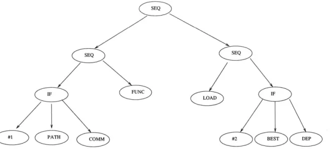
SEQ

SEQ SEQ

IF ~ FUNC I

LOAD

COMM #2 BEST DEP

Figure 4-2: Sequence of passes coded as an s-expression. The s-exp represents a se-quence that runs (PATH) or (COMM), then (FUNC) and (LOAD), and then (BEST) or (DEP), according to the results computed by the metrics.

Chapter 5

Compiler Infrastructure

In this chapter, we describe our compiler infrastructure and how we integrated con-vergent scheduling into Raw and Chorus. We also describe the scheduling algorithms we used for comparison in our experiments.

5.1

Chorus Infrastructure

The Chorus clustered VLIW system is a flexible compiler/simulator environment that can simulate a large variety of different configurations of clustered VLIW machines.

In chapter 6, we use it to simulate a clustered VLIW machine with four identi-cal clusters. Each cluster has four functional units: one integer ALU, one integer ALU/Memory, one floating-point unit, and one transfer unit. Instruction latencies are based on the Mips R4000. The transfer unit moves values between register files on different clusters. It takes one cycle to copy a register value from one cluster to another. Memory addresses are interleaved across clusters for maximum parallelism. Memory operations can request remote data, with a penalty of one cycle.

Nonetheless, most of these parameters can be changed in our infrastructure. We tested the robustness of convergent scheduling to these changes in chapter 7.

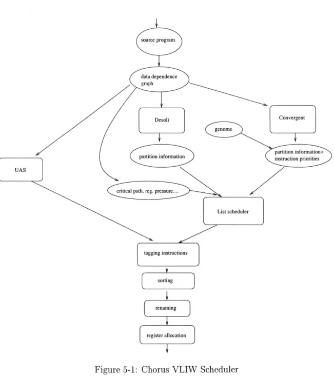
As part of the Chorus infrastructure, we developed a flexible VLIW scheduler, seamlessly integrated with the rest of the system

[MazO1].

The system (see figure 5-1):

" reads in the program, and build the dependence DAG for every block;

" determines the best space-time scheduling for the instructions in the block;

different algorithms are used and compared;

" tags instructions with the chosen space/time schedule;

" sorts instructions so to be in the correct final sequence;

" creates new names for the temporary registers used in clusters different from

the first and corrects the instructions using the new names;

" performs register allocation.

Register allocation is performed by MachSuif Register Allocator (based on George and Appel's work [GA96]), modified by our group to manage multiple clusters and predication. The code is then finalized and simulated on our step-by-step simulator. In this work, three algorithms are implemented and tested. Convergent scheduling is the first. As a comparison, we implemented Desoli's PCC algorithm for clustered

DSP architectures [Des98], and the UAS algorithm [OBC98].

5.1.1

Partial Component Clustering (PCC) algorithm

imple-mentation

Our system implements Desoli's Partial Component Clustering (PCC) algorithm, as in [Des98]. We try to illustrate our implementation here in detail.

Our algorithm builds the sub-components, as described in the paper. Then, it initially assigns them so to balance the load in different cluster. As in the origi-nal implementation, we iterate the initial assignment changing the size of ith (the maximum size of a sub-component) to minimize the expected schedule. This is done using a simplified list scheduler, more details about which are below. In the paper, the way that the various values of

#th

source program

data dependence graph

Desoli Convergent

partition information pintution ioriaties+_{instrction priorites}

UAS

critical path, reg. pressure....

List scheduler

tagging instructions

sorting

renaming

register allocation