Contact angle hysteresis: a review
of fundamentals and applications
The MIT Faculty has made this article openly available.
Please share
how this access benefits you. Your story matters.
Citation
Eral, H. B., D. J. C. M. ’t Mannetje, and J. M. Oh. “Contact Angle
Hysteresis: a Review of Fundamentals and Applications.” Colloid
Polym Sci 291, no. 2 (February 2013): 247–260.
As Published
http://dx.doi.org/10.1007/s00396-012-2796-6
Publisher
Springer-Verlag
Version
Author's final manuscript
Citable link
http://hdl.handle.net/1721.1/86387
Terms of Use
Article is made available in accordance with the publisher's
policy and may be subject to US copyright law. Please refer to the
publisher's site for terms of use.
1
Contact angle hysteresis: A review of
fundamentals and applications
H.B. Eral*¥, D.J.C.M. ’t Mannetje* and J.M. Oh
Physics of Complex Fluids, TNW, University of Twente, P.O. Box 217, 7500 AE, Enschede, The Netherlands Abstract:
Contact angle hysteresis is an important physical phenomenon. It is omnipresent in nature and also plays a crucial role in various industrial processes. Despite its relevance, there is a lack of consensus on how to incorporate a description of contact angle hysteresis into physical models. To clarify this, starting from the basic definition of contact angle hysteresis, we introduce the formalism and models for implementing contact angle hysteresis into relevant physical phenomena. Furthermore, we explain the role of the contact angle hysteresis on physical phenomena relevant for industrial applications such as sliding drops, coffee stains phenomenon (in general evaporative self-assembly), curtain and wire coating techniques.
Keywords: Contact angle hysteresis, sliding drop, coffee stain, coffee ring, mechanical reduction of contact angle hysteresis, electrowetting, pattern formation, evaporative self-assembly, advancing and receding contact angle
*indicate equal contribution
2
1.INTRODUCTION
Contact angle hysteresis (CAH) is one of the most important and classic elements of wetting of liquid droplets in systems from centimeter to micrometer scales. It is perhaps most intuitively understood by looking at a droplet resting on a horizontal substrate (Fig. 1 a): Similar to a rain drop on a window. Gravity pulls on the droplet to move it down, while CAH will keep the droplet in place. As a result, droplet will become asymmetric but will not move: the top of the droplet becomes thin, with a low contact angle, while the bottom becomes thick, with a high contact angle. If the droplet reaches a certain size, it slides down in an asymmetric shape, and the difference between its front (in the direction of driving force in this case gravity) and back contact angles (in the direction opposing the driving force) is called the contact angle hysteresis [1-7].
Figure 1: a) a drop on a vertical surface, stuck at the critical advancing angle θa and the critical receding
angle θr. b) By slowly pumping liquid into or out of a sessile droplet, both the advancing and receding
angles can be readily measured.
Other occurrences can be seen in coating processes (dynamic hysteresis), digital microfluidics and evaporation of droplets (leading to the well-known coffee stain). Industrial applications where CAH plays a role include immersion lithography, fiber coatings, and ink-jet printing. In these, it is clear that in some cases, hysteresis is a problem (immersion lithography) while in others it is essential (dip-coating). Determining and controlling CAH are critical for the operation of these industrially relevant systems.
3
Given its great practical value, many scientists have studied the source and effects of hysteresis. De Gennes in his 1985 review [3] delves into some of the historical experiments done in the early 20th century, but overall the study of hysteresis, and its effects on the motion of liquids, has especially received attention since the 1950’s [8-11]. From the specific subject of spray retention for agricultural purposes, Furmidge in 1962 [12] came up with a simple formula to describe the retention of droplets on inclined planes, while Bikerman in 1950 [13] showed the equilibrium situation for a water droplet sliding at constant velocity on different surfaces with different roughness levels. The work of Dussan in the 1980’s [2, 14, 15] built on this basis, to give a theoretical understanding of the retention forces on droplets sticking to solid surfaces.
However, this work did not for the most part emphasize the effect of motion. In 1971, Huh and Scriven famously stated that “not even Herakles could sink a solid if the physical model were entirely valid” [16] as the shear stress approaches infinity when one comes close to a moving solid-liquid-fluid contact line. Here the physical model is simply hydrodynamics, with the no-slip boundary condition. As we know from our intuition, a solid can be immersed in liquid which requires that the contact line moves. A moving contact line is a violation of the no slip boundary condition evoked in hydrodynamic models, it is clear that a different model or boundary condition must be used to describe the motion near the contact line. Blake and Haynes [17] proposed that a different model should be used, based on the motion of the individual molecules near the contact line, rather than on bulk hydrodynamics. The model is called the molecular-kinetic model. A competing model is based on a relaxation of the no-slip boundary condition, while otherwise using continuum theory; Voinov in 1976 [18] and Cox in 1986 [19] are now most famous for the development of this hydrodynamic model, and its prediction captured in the Cox-Voinov law. Both models describe a large increase in the hysteresis as a
consequence of contact line motion, which fits with experiments. However, the two models give quite different predictions of how the hysteresis will increase, yet both make physical sense. Recently, phase field modeling was also adapted to hysteresis [20, 21].
In the last decades many experiments as well as analytical and numerical calculations have focused on resolving which model is more accurate, or when it is better to use one or the other, but as seen from a recent special issue of the European Physical Journal (Volume 197, Number 1 / August 2011) the question is far from settled.
In this review article, we start by defining contact angle hysteresis. This is followed by an introduction of the formalism and the theoretical models for contact angle hysteresis are explained under three categories Hydrodynamic, Molecular-Kinetic and Combined models. We shed light onto the lack of consensus regarding these models in Section 3. Following the theory section, we will introduce a set of
4
physical phenomena where contact angle hysteresis plays a crucial role and explain the advantages of manipulating the contact angle hysteresis in Section 4. The introduced physical phenomena aims shed light on the effect of CAH on the working principles of industrially relevant physical phenomenon including sliding drops, coffee stain phenomenon, curtain and fiber coating.
5
2. CONTACT ANGLE HYSTERESIS MEASUREMENT
2.1 Definition of contact angle hysteresis
For the purpose of this review, we define the contact angle hysteresis as the difference of the
advancing contact angle and the receding contact angle for a contact line moving in opposite direction at the same velocity.
As sketched in Fig. 2 one can see that this difference in fact consists of two parts. First, there is a jump in the contact angle at zero velocity. This jump, known as the contact angle hysteresis in some other publications, is the difference in contact angle induced by surface effects, such as roughness and heterogeneity. It can be seen as the difference between the maximum (advancing) and minimum (receding) contact angles for which a (local) minimum exists in the Gibbs free energy [22]. While these angles are not fully stable, the energy barriers to reach the minimum in the free energy are usually so large that only the advancing and receding angle are seen. A caveat is that the theoretical advancing and receding angles also have the lowest energy barrier, in general, so a slight vibration may shift the angle to a minimum closer to the global minimum in energy (so that the experimentally found hysteresis may be lower than the theoretical one), but rarely to the minimum itself. The static hysteresis is extremely stable, i.e., a droplet can be deposited in a state where it maintains a contact angle between the two limiting angles, without relaxation or motion (assuming no evaporation occurs). However, there is a retention time dependence of contact angle hysteresis due to deformations of the substrates induced by the unbalanced surface normal component of the surface tension [23]. An important point to note is that this static hysteresis is purely based on the surface directly underneath the contact line. For sufficiently long contact lines over random surfaces, using an average over the liquid-solid interface will be acceptable. For very large structures, however, this point is critical [22, 24, 25].
The dynamic component of the hysteresis is caused by the interplay of the liquid motion with the solid surface, and especially the liquid’s inability to simply flow over it. For a slow-moving drop on a rough surface (that is, all solids but single crystal structures like mica/graphene) the static hysteresis will dominate, but for high velocities or low static CAH surfaces (especially on liquids or liquid-soaked solids) the dynamic hysteresis becomes extremely important. Notably, there will be a clear velocity dependence of the contact angle even for cases with only a single contact line (such as, say, a plate plunging into a bath of liquid), while the static part of the hysteresis will be essentially invisible.
6
The hysteresis as defined here is thus the sum of the static hysteresis, the dynamic increase of the advancing contact angle, and the dynamic decrease of the receding angle.
Figure 2: Schematic of contact angle hysteresis: at 0 velocity there is already a difference between the advancing (right of axis, for a contact line moving out of the liquid) and receding (left, for a contact line moving into the liquid) angles, called the static hysteresis, and this difference increases with increasing capillary number (Ca). This increase we call the dynamic contact angle hysteresis. Capillary number is defined as the ratio of viscosity (η) and velocity (U) to liquid vapor interfacial tension (γlv).
2.2 How to measure the contact angle hysteresis?
Experimentally, static CAH can be determined by three methods [26-30]. The first method is tilted plane method where a droplet is placed on an inclined plane and its contact angles are measured when it starts sliding down (see also Fig. 1 a). A modification of the tilted plate method is the centrifugal force balance method. This method allows for decoupling of the tangential and parallel components of the adhesion force. It makes use of centrifugal force to separately control the lateral and tangential forces for droplets as they rotate on an inclined plane [31]. A second method is the sessile drop method or the captive bubble method, whereby liquid (gas) is pumped into and out of a droplet (bubble) to achieve first the advancing and then the receding angles (Fig. 1 b). A modification of the sessile drop method is the evaporation method [29, 32, 33], where the receding angle is measured as a droplet evaporates. A third method that is often used is a Wilhelmy method, where instead of the droplet moving over the surface, a surface is lowered into a bath or pulled out of it to achieve the advancing and receding angles, respectively.
7
What these methods share is relative simplicity; the tilted plate method requires only a camera, the sessile drop method (usually) additionally needs a needle and a pump, while the Wilhelmy method requires only a motor and force measurement device. However, all three have their share of disadvantages.
In the tilted plate method, there are some minor concerns: first, the droplet has to move at a finite velocity, which can at times create problems in optical measurements. Second, and usually more critical, is the change in pressure between the front and back of the droplet leading to a strong or weak curvature, respectively. While the contact angles themselves will not change, most optical
measurement methods require a fitting of the liquid-air interface profile; the curvature of this interface may thus affect the fitted contact angle. However, a much larger issue raised by Krasovitski and Marmur [34] is that, in some cases, the droplet may begin to move while the advancing or receding angles are not reached. Moreover, Pierce et al. [35] showed that the placement of the droplet, and the resulting droplet shape, could have a significant influence on the resulting minimum angle for drop sliding. Therefore, while it remains an excellent qualitative way to distinguish between a high-hysteresis surface, where droplets tend to stick, and a low high-hysteresis surface, where they tend to slide down easily, and recent literature rarely focuses on this method. The newly proposed centrifugal force[31] balance may aid in bringing this method back into focus, as it allows measurements for different drop volumes at the same inclination angle. This may improve the reproducibility, while also allowing the decoupling of the lateral and tangential forces on the droplet, which change
simultaneously for a changing angle of the inclined plane. Between the Wilhelmy and sessile drop methods, as seen in recent discussions [26-28] there is no clear consensus which method is better, and indeed both have advantages and disadvantages.
The sessile drop method is often used for its ease of comprehension and visual clarity; i.e. the method uses optical imaging to show contact angles. Thanks to this optical nature of the sessile drop method, Buehrle and coworkers [36] showed that in electrowetting only the apparent contact angle changes while the Young angle stays constant. This is a situation where the sessile drop method offers a great advantage, although strictly speaking it is used to determine an interface shape rather than a real contact angle.
Also, in contrast to the Wilhelmy method, the sessile drop method can be used on any patch on a larger surface. It is simply a matter of placing a small droplet on the area to be measured. This also
8
avoids any issues with surfaces where edges are a significant element of the production process but are irrelevant to the actual experiment. However, in other experiments, where the wetting properties of a larger surface are of interest, this advantage can become a disadvantage. The Wilhelmy method will average over a large surface and measure wettability quickly, while the sessile drop method would require many series of experiments on different locations to properly characterize the entire surface.
A second big advantage of the sessile drop method is that it directly measures a contact angle, while the Wilhelmy method measures the force resulting from this contact angle. On a smooth surface this is no problem, but on a rough surface the actual length of the contact line between the liquid and surface will determine the force, which may be difficult to obtain; the sessile drop method will still show the contact angle readily, though it must be regarded as an ‘effective’ contact angle while the actual contact angle may vary locally.
A perhaps much larger practical advantage of the sessile drop method is its ability to function on a single surface; the Wilhelmy method requires a plate plunged into a bath, and so the surface should be the same on all sides. The sessile drop method, however, can be used on surfaces that have been modified on one side. While this concern can be somewhat reduced by sticking two prepared surfaces together, this is evidently not the most practical situation. Edge effects will also become more
important, as the sides will become twice as thick.
There are, however, some critical problems with the sessile drop method. The first of these is the use of the needle in sessile drop experiments. This may distort the droplet shape and thereby the observed contact angle; this is especially true for surfaces with large hysteresis, as the needle must be in contact with the droplet over the entire range of angles. A second major issue is shared with all optical
methods: when the contact angle approaches 0 or 180 degrees, it becomes nearly impossible to see the exact point where the droplet ends and the surface begins. Using more advanced analysis techniques it may still be possible to extract contact angles from the shape of the droplet [37], but simply fitting the liquid-air or liquid-liquid interface will result in large errors in contact angle determination. On the other hand, the Wilhelmy method is still quite valid for extreme contact angles. In some cases the captive bubble approach, which inverts the liquid and gas phase, can be a useful alternative to the sessile drop method. A drop on a hydrophilic surface i.e. contact angle that is approximately zero degrees is often easier to measure than the one close to 180 degrees. Converting the method of
9
et.al. [30]. A larger part of the surface will be wetted than in the sessile drop method, but usually it will be possible to avoid wetting the sample edges.
2.3 Hysteresis and Young’s angle
Many authors have studied ways to relate the contact angles on surfaces with Young’s angle and the interfacial tension of a surface-liquid interface. Recent works have focused on finding the most-stable contact angle by, for example, vibrating the droplet or surface [38-40] which was already shown to be a way to reduce the difference between advancing and receding angles [41, 42]. Others seek to calculate this angle from advancing and receding angle data [43, 44] by a theoretical approach.
10
3. Theories of Contact Angle Hysteresis
In this section, the models for describing the behavior of the contact angle in the presence of
contact line motion, as well as models for static contact angle hysteresis and their
implementation is discussed. This discussion is of utmost importance in understanding the
influence of contact angle hysteresis on the physical phenomena discussed in Section 4.
3.1. Dynamic contact angle models
Young's equation defines the relation between interfacial tensions and the equilibrium contact
angle
Y[45].
LV SL SV Y
cos (1)
where
LV,
SVand
SLrefer to the liquid/vapor, solid/vapor, and solid/liquid interfacial
tensions, respectively.
Boruvka & Neumann [46] modified the Young equation to take into account the three-phase
contact line tension
LV Y Y Κ
cos cos ' (2)
where
the contact is line tension and
Κ is the curvature. The contact angle represents the
angle tangent to the drop surface measured from the substrate surface at the three-phase
contact line (TCL). The apparent contact angle should be distinguished from the microscopic
contact angle, i.e. Young's angle. When an electric field is applied to a conducting drop on a
substrate coated with a dielectric layer, the apparent contact angle is affected by the electrical
stress formed near the TCL, which is referred to the electrowetting (EW) [47]. The
Lippmann-Young equation predicts accurately the equilibrium contact angle in EW until
saturation of the contact angle occurs:
LV Y Y
d
V
2
cos
cos
2 0 '
(3)
11
where
0,
, Vand
dare the electrical permittivity in vacuum, the dielectric constant, the
applied electrical potential and the dielectric layer thickness, respectively. Now, we discuss
the models associated with dynamic contact angles and energy dissipation originating from
movement of the contact line.
3.1.1. Hydrodynamic model
The hydrodynamic model assumes that the moving process of the contact line is dominated by
the viscous dissipation of the liquid, which implies that the bulk viscous friction is the main
resistance force for the contact line motion [18, 19]. The model separates the liquid into an
inner region and an outer region, sometimes even with an intermediate region. In the outer
region, the conventional ''no-slip'' boundary condition is applied, while in the inner region, the
fluids slip within a couple of molecular layers adjacent to the solid surface. From the
lubrication theory with the assumption that the flow profile is nearly parabolic in the liquid
phase, one can derive the Eq. (4).
''
'
Ca
3
2h
h
(4)
where
his the position-dependent height of the liquid and the capillary number is defined by
LV
U
/
Ca
with moving velocity
U, the viscosity
and the surface tension
LVof the
liquid. Here, the prime (‘) presents the derivative with respect to x -direction parallel to the
substrate. Voinov derived the solution of Eq.(4) with a vanishing slope at infinity [3] given in
Eq.(5).
s mL
x
x
h
'
3(
)
39
Ca
ln
(5)
Here,
mis the equilibrium contact angle and
L is the slip length. Eq. (5), or its variation, is
susually referred to as the Cox-Voinov law [19]. Cox extended Eq. (5) to two fluids with
viscosity ratio
M
out/
12
s mL
x
M
g
M
x
g
(
(
),
)
(
,
)
Ca
ln
(6)
where
tan
h
'
(
x
)
. When there is no outer, dynamically active fluid,
g
(
(
x
),
0
)
reduces to
)
(
g
, defined by
xdx
x
x
x
x
g
02
sin
cos
sin
)
(
(7)
which cannot be integrated in a closed form. The model can be well approximated by the
relation
s m dL
x
ln
9Ca
3 3
(8)
where
L is the characteristic capillary length [48]. This model is valid under the conditions
where Reynolds number (Re) and the Capillary number (Ca) are less than one: Here the
Reynolds number is defined as the ratio of inertial forces to viscous forces where ρ, U, η are
density, velocity, viscosity of the liquid and L is the characteristic dimension, respectively.
UL
Re
and
Ca1 (9)The slip length
L is, in practice, the fitting parameter and represents the length of the region
swhere no-slip boundary condition does not apply. Therefore,
L
sshould be of the order of
molecular dimensions. According to the experimental observations, the hydrodynamic model
is mostly satisfactory in small contact line velocity regime [49]. The main limitation of this
model is that it does not take into account the characteristics of the solid surface [19, 50, 51].
3.1.2. Molecular-Kinetic model
Yarnold and Mason (1949) suggested that
U
(
)
could be controlled by adsorption/desorption
processes very near the contact line [52]. Later, Blake and Haynes transformed this idea into a
quantitative theory [17]. In contrast to the hydrodynamic model, the Molecular-Kinetic model
13
neglects viscous dissipation and takes the solid surface characteristics into account. According
to the Molecular-Kinetic model, the motion of the contact line is determined by the statistical
dynamics of the molecules within a three-phase zone where the solid, liquid and gas phases
meet. The important parameters are
0, the equilibrium frequency of the random molecular
displacements occurring within the three-phase zone, and
, the average distance between the
adsorption/desorption sites on the solid surface. The model assumes that the velocity
dependence of the dynamic contact angle originates from the disturbance of adsorption
equilibrium and to changes in the local surface tension as the wetting line moves across the
solid surface. Then, the driving force for the contact line to move is given as
m d
LV W
F
cos
cos
(10)
The resulting equation for the wetting line velocity is then
k T
U( ) 2 sinh LV cos m cos d /2 B
2
0
(11)
where
k is the Boltzmann constant and
BT the absolute temperature. A rearrangement of Eq.
(11) gives [7, 15]
1 0 22
sinh
2
cos
cos
k
T
U
LV B m d (12)
Eq. (12) gives a good fit to the set of data provided by Blake, in particular in regimes of rather
high velocity. Here,
0and
are fitting parameters just like the slip length in the
hydrodynamic model, which implies that both approaches are not self-contained [48].
3.1.3. Combined model
In many experimental observations, it is shown that neither the hydrodynamic model nor the
Molecular-Kinetic model satisfies the entire velocity range. So, it is natural to try a model in
which both wetting line friction and viscous dissipation play a part in determining the
dynamic contact angle [19, 53, 54]. A combined molecular-hydrodynamic model [53] can be
derived by combining Eq. (7) and (12).
14
s LV B m dL
L
U
T
k
ln
Ca
9
2
sinh
2
cos
cos
3 0 1 2 1 3
(13)
Note that
,
0 andL are, in practice, the fitting parameters even though they have their own
sphysical meanings. Petrov and Petrov (1992) [53] and Brochard-Wyart and de Gennes (1992)
[4, 55] developed more or less the same model with different approaches. The combination of
the Molecular-Kinetic and conventional hydrodynamic model gives us an understanding on
the real physics of wetting/dewetting dynamics. However, the combined model is still
phenomenological, and we use several fitting parameters in the name of physical
interpretation. And, the combined model is valid only in the low capillary number regime.
3.2. Contact angle hysteresis models
Eqs. (1) and (2) describe the equilibrium contact angle on a smooth, chemically homogeneous
surface. For heterogeneous surfaces, the equation for the equilibrium contact angle can be
expressed as the Cassie [56] equation
B Y B A Y A C Y
f
f
cos
cos
cos
(14)
where
is the area fraction of the component surface satisfying
A
B
1
f
f
. On the other
hand, for a rough homogeneous surface, Wenzel derived the equation
Y W
Y
r
cos
cos
(15)
where
ris the roughness factor (ratio of the surface area to the projected area of the surface)
[57, 58]. Equation (15) may misleadingly give the idea that the contact angle is determined
solely by the area fraction. As commented by Panchagnula and Vedantam, it is rather
determined by the conditions near the contact line [20]. Even if the area fraction along the
contact line is kept constant, the contact angle may change with respect to the contact line
topology [59, 60].
It is very difficult experimentally to measure the equilibrium contact angle even for smooth
homogeneous surfaces. The measured contact angle is usually in between the receding and
advancing angles
rand
arespectively. The advancing and receding angles are empirically
15
reproducible and the contact angle hysteresis (CAH) can be expressed as
a
r. The
origin of CAH has been debated vigorously for a long time. Most theoretical models have
focused on surface roughness and heterogeneities as a source of CAH. They developed
models for idealized surfaces such as surfaces with parallel grooves or axisymmetric grooves
[61, 62]. After this, the pinning phenomenon due to randomly distributed defects was studied
based on a statistical approach [1, 63, 64]. A thermodynamic model combining surface
roughness and heterogeneities has also been suggested [65]. Roughness, chemical
heterogeneities, surface deformation, liquid adsorption and retention, molecular
rearrangement on wetting, and interdiffusion can be other factors [3]. Especially, Yang [66]
and Extant [67] showed that the irreversible adhesion and separation events which occur
during advancing and receding processes can contribute to CAH. It was also reported that the
CAH is related to a stick-slip mechanism which depends on the disorder and the size of the
system.
Whyman et al. derived the contact angle hysteresis model based on a simple thermodynamic
model [68]
4 / 1 * 3 / 1 3 / 2 * 12 / 1 * 2 / 1 0 2 (1 cos ) ) cos 2 ( ) cos 1 ( 8
R U LV r a(16)
where
*is the apparent contact angle at equilibrium.
Walker and coworkers derived a phenomenological model for a dynamic contact angle model
with pinning pressure to take the hysteresis into account [69].
U c c U c U pin pin pin m d LV ) 2 / /( tan 2 / ) sgn( cos cos 1
(17)
where
and
cpinare the friction factor and the pinning pressure, respectively. Combining the
Lippmann-Young equation and Eq. (15), Oh and coworkers used the dynamic contact angle
model to analyze the drop spreading based on the normal mode analysis [70].
16
3.3 Numerical implementation of dynamic contact angle model
There are two distinct approaches in numerical simulations involving dynamic contact angles:
one is the continuum approach such as lubrication theory and the diffuse interface model and
the other is the molecular approach such as molecular dynamics simulation and
lattice-Boltzmann simulation. In the continuum approach, most do not describe the microscopic
interactions between the fluids and the solid wall but solve the flow field on a macroscopic
scale. The limitation of such an approach is that it is not possible to relate the macro flow field
directly to the molecular scale responsible for the wetting. Meanwhile, in the molecular
approach, simulations are restricted to small systems (such as a drop of few tens of
nanometers in size) and, as a consequence, the results are subject to significant thermal and
statistical fluctuations.
In the continuum approach, a proper treatment of the wall boundary condition is crucial to
avoid the stress singularity at the contact line. One remedy is the Navier condition for the
velocity component along the entire wall
x
U
l
U
c
(18)
where
l is the slip length[19]. Alternative approaches are to include microscopic (van der
cWaals) interactions between the fluids and the solid wall or a precursor film ahead of the
moving contact line, or to use a diffuse interface. In addition to the Navier condition, the
contact angle or contact line speed must be prescribed, which is the dynamic contact angle
model including hysteresis. In numerical simulations, a simplified model is used in many
cases[71]. One of the limitations in this approach is that the slip length is proportional to the
grid spacing, irrespective of physical dimension [72, 73].
Molecular dynamics (MD) is a different way of doing numerical “experiments” at molecular
level detail [74-76]. As a computing power has increased in recent years, larger scale MD
simulations have been investigated for spreading liquid drops, capillary filling and dynamic
wetting on curved surfaces [54, 77-80]. They show that the equilibrium contact angle (
m) is
17
3.4 Summary of theoretical models
There are two different approaches to explain the dynamics of the moving contact line on the
substrate. One of them (hydrodynamic model) assumes that the viscous dissipation in the bulk
phase is dominant and the other (Molecular-Kinetic model) focuses more on the
adsorption/desorption processes between liquid and substrate molecules. The combined model
to cover a large velocity range is also suggested, but still has limitations in applicability and
its validity depends on the situations such as physical properties of the liquid and substrates.
The origin of the contact angle hysteresis has been debated for a long time and it is suggested
that surface roughness, chemical heterogeneities, surface deformation, liquid
adsorption/desorption, molecular rearrangement and etc. can be some important causes.
However, there is no concrete consensus and full understanding on the hysteresis
phenomenon on smooth and chemically homogeneous surfaces, yet. Some numerical
investigations including MD simulations have been tried to understand the hysteresis
phenomenon at molecular level, but there are restrictions in size and time-limit problems due
to high computing power required.
18
4. APPLICATIONS AND RECENT PROGRESS IN MANIPULATION OF
CONTACT ANGLE HYSTERESIS
As we previously mentioned contact angle hysteresis manifests itself in various aspects either as the underlying physical mechanism of industrial processes that directly influence our daily life. We will discuss a few examples where controlling\manipulating the contact angle hysteresis stands at the heart of these processes. In this section, recent progress and tools to manipulate contact angle hysteresis in sliding droplets, coffee stain phenomenon and climbing droplets are discussed along with processes which might benefit from manipulation of contact angle hysteresis such as curtain and wire coating.
4.1 Control of contact angle hysteresis by Electrowetting: Sliding drop and Coffee stain
In this section, we will introduce two physical phenomena relevant for industrial processes: Sliding droplet and Coffee stain formation.
4.1.1. Sliding droplet
Droplets stick to surfaces in many applications, due to contact angle hysteresis [6]. A classic example is a droplet on an airplane or car window obscuring vision, or the sticking of pesticides to leaves. For a droplet on a surface driven by gravity the onset of motion has been described for several decades. Early experiments are due to Bikerman and Furmidge [12, 13], and the theoretical discussions flared up since the work of Dussan in the 1980’s [2, 15], with experiments and theoretical descriptions continuing up to the present day [34, 35, 67, 81-87].
The basic setup is quite simple, as already shown in Fig.1 a in the Introduction: a small droplet sticks to a surface due to hysteresis. However, for the sliding of a droplet the shape of said droplet and especially its width are also critical.
In principle, the sliding of a drop over a surface [87] is extremely similar to that of a drop held between two surfaces; however, the resulting droplet geometry can be very different [85] as the confinement changes the possible droplet shapes. Still, the resulting formulas to describe drop motion are remarkably similar.
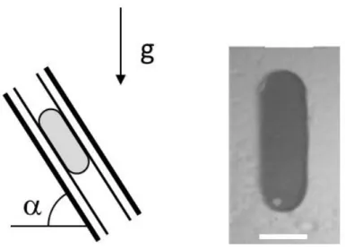
19
Figure 3: The panel on the left shows a schematic picture of a droplet held between two surfaces under gravity. The two surfaces can be tilted to some angle α, thereby changing the effective gravitational force. The advantage of the two-plate geometry is seen in the real picture on the right: the drop remains in an approximately ellipsoidal shape up to high velocities, while on a single surface it will soon develop a tail that eventually leaves behind droplets, the so-called pearling transition [87]. The white scale bar (5 mm) is approximately the width of the droplet, which, besides the contact angle hysteresis, proves to be a critical parameter in this system
Before the onset of pearling, as well as for drops between two plates, the shape of these droplets on the surface is most simply approximated by two semicircles connected by straight edges; only for a zero-hysteresis surface a droplet can move with a spherical footprint.
The most important issue for most applications is determining the threshold of motion, and linked to that is the velocity of a given droplet above the threshold. The equation to determine the resisting force for each surface due to hysteresis for drops with this semicircle-straight shape is [2]:
) cos
(cos R A
p w
f
(19)
In this equation, w is the width of the droplet and is the surface tension. The work by ElSherbini and Jacobi [82] shows some of the modifications to this simple equation, based on various methods to more closely approximate the real force induced by the contact line. Due to the relative simplicity of measuring the width and shape of the droplet these better approximations are certainly valuable, but the resulting change in pinning force is not very large. Tadmor [88] argues that the actual dependence
20
is not on the width itself, but is due to the experimental procedures of a tilting plate. This does appear to be the case; however, for practical purposes Eq. (19) is a useful approximation.
The sliding threshold is a simple matter of balancing the gravitational driving force with the resisting force of Eq. (19), and indeed it can also be applied to drops sliding in micro channels, where the driving force is completely different. In all cases, the pinning force scales with the hysteresis, and so controlling the hysteresis could be useful. Simply having droplets roll off a car window, rather than needing a wiper system, could then be possible.
A recently developed way to control the hysteresis is by AC electrowetting. As described in the beginning of this section, the hysteresis of a conducting droplet can be reduced by rapidly shaking the droplet using an electric field that rapidly turns on and off (i.e. an AC signal) [85, 89]. In either a two plate system, or using so-called interdigitated electrodes, the actual hysteresis force can be reduced, and drops mobilized. Of course, being an electric signal, it is also possible to turn it on and off, allowing exact control of a droplet close to the sliding threshold, sliding when the voltage is applied, and stuck when it is not.
4.1.2 Coffee stain phenomenon: Contact angle hysteresis in evaporative self-assembly
A specific example of the influence of the contact angle hysteresis on pattern formation in processes is the coffee stain phenomenon. An evaporating droplet containing a nonvolatile component leaves behind a heterogeneous solid residue (Fig. 4). Despite the fact that we all have seen them, only few of us with a keen eye realize the common feature of these solid residues named after its most commonly encountered example: coffee stains. Deegan and coworkers [90, 91] explained how nature creates coffee stains. Various nonvolatile materials such as solid particles with sizes ranging from hundreds of microns to a few nanometers, polymers, even various biomolecules such as DNA or proteins form similar patterns upon evaporation on a flat substrate. In their seminal study, Deegan et al. explained that the formation of a coffee stain occurs through two factors (i) the contact angle hysteresis and (ii) the evaporation driven capillary flow pulling the contents of the droplet towards contact line. When the contact line pins, a wedge-like shape is formed (Fig. 4). This wedge-like shape creates the
aforementioned evaporation driven capillary flow. In other words, close to the periphery of the droplet where the droplet is thinnest the evaporation rate becomes dramatically higher. This locally high
21
evaporation rate sucks particles to the contact line with a capillary flow. This capillary flow towards to contact line is the reason why we observe the coffee stains. As a drop evaporates with the contact line pinned, the particles accumulate and jam [92] near the contact line, further strengthening the pinning. CAH or pinning of a moving contact line has been used extensively in evaporating assembly [93], particularly in micro and Nano patterned three dimensional structures [94, 95]. Yet, only a few have evoked the idea of controlling the CAH to control pattern formation [96].
The two underlying factors according to the Deegan scenario can be rationalized through thinking about our daily experiences. First, contact angle hysteresis can be visualized easily by thinking of a rain drop sliding on a tilted window. On a very smooth window surface, the droplet will slide down gradually. If the surface is rougher i.e. full of scratches and cracks, the droplet will stick, in other words the contact line will pin and not move. As expected the rougher the surface (i.e. The higher the density of scratches and cracks), the easier the drop will pin. When a sessile droplet on a horizontal surface evaporates the contact line tends to move inwards over the aforementioned cracks and dents. If finally the contact line pins due to this roughness, the shape of the drop at the rim becomes wedge-like (Fig. 4). It is also important to realize that contact line pinning is not only due to roughness but also the particles (in general nonvolatile component) confined at the three-phase contact line contributes to the pinning. This is often an overlooked aspect connecting coffee stain phenomenon to confinement induced glass transition in colloidal systems [92, 97, 98] and dynamics in the vicinity of grain boundaries [99-101].
Second, due to the wedge shape of the evaporating droplet, the local evaporation rate (J) increases towards the edge. This is simply because at the rim an evaporating molecule has a larger free space available than in the central region of the drop where it has to compete with more evaporating molecules for that free space. In other words, close to the periphery of the drop the evaporation rate increases provided that the evaporation is diffusion limited. Furthermore, from our daily experience we know that evaporation can be enhanced by increasing the available area. Imagine the evaporation in a glass of water; if we pour the water from the glass over a flat surface the water will be gone much faster. As the evaporation is higher at the edge of the drop than in the bulk, both liquid and particles are sucked towards the contact line. From Fig. 4, it is rather straightforward to see that the higher evaporation near the rim leads to a net flow towards the contact line. Due to this outward flow the nonvolatile particles accumulate near the rim and that is why we observe the coffee stain. Despite the fact that this explanation ignores a lot of details like particle-surface interactions, it describes the phenomena quite well. Recent works have shown that arrangement of particles is influenced by the strength of capillary flow i.e. how fast particles go to the contact line [102, 103].
22
Figure 4: Illustration of coffee stain formation in Panel (a) and a microscope image of a coffee stain formed by fluorescently labeled 5 µm particles in Panel (b).
Why is coffee stain a problem?: Coffee stain phenomenon can be a real undesired nuisance and a limiting physical factor for a large family of industrial processes involving nonvolatile components dispersed in evaporating solvents such as inkjet printing of circuits, OLED displays, or drying of paint. In all of the above applications, a homogeneous distribution of the nonvolatile component is required. Lack of such a homogeneous distribution caused by coffee stain phenomena leads to undesired efficiency loss. A specific example of these industrially relevant applications where a coffee stain is not desired is encountered in the analytical detection of biomolecules with the microarray and MALDI-MS techniques. For these bioanalytical techniques, repeatability and consistency are at the heart of the process and that is where the coffee stain effect strikes, compromising the efficiency of the process. For optimal efficiency the molecules should be distributed homogeneously over the dot, but in practice they end up predominantly on its rim due to the above described coffee stain effect. Hence suppression of this stain effect would greatly improve the efficiency of the detection process.
According to the Deegan scenario by controlling contact angle hysteresis [89] or counteracting capillary flow [96], we can control/avoid coffee stain formation. Electrowetting [47] is a tool that can provide these two aspects simultaneously (Fig.5).
23
Figure 5: Demonstration of the coffee stain effect of an electrowetting (EW) based method for suppression of Coffee stain effect. The “No EW” branch demonstrates evaporation of a drop containing solid particles on a solid surface with no interference. Capillary flow induced by contact line pinning and the inhomogeneous evaporation pushes the particles towards the contact line. Particles pushed along the contact line create an inhomogeneous distribution. When our method is employed, the coffee stain effect is suppressed. Simultaneous suppression of pinning and the production of mixing patterns that counteract the capillary flow are achieved. Red arrows indicate the flow patterns.
In a recent communication, we demonstrated that the formation of coffee stains can be suppressed by applying electrowetting (EW) with an alternating voltage to evaporating drops containing a wide range of colloidal particles and cDNA [96]. The suppression of the coffee stain by electrowetting can be explained with the scenario proposed by Deegan et al. In this aforementioned scenario, the coffee stains are created due to contact angle hysteresis and capillary flow. EW creates an electric force that disturbs the force balance at the contact line (Fig. 5). Electrowetting with AC frequency alternatively increases and decreases the apparent contact angle essentially depinning the contact line i.e. not allowing it to get stuck to intrinsic roughness features on the surface. This can be interpreted as modulation of CAH [89].
Furthermore, by choosing the frequency of the applied field appropriately, the drop surface can be brought in an oscillatory motion. Due to these surface oscillations an internal flow is created which counteracts the capillary flow induced by the evaporation process and the non-volatile particles do not migrate to the contact line anymore, eliminating the second condition, too. In this way we are able to suppress the coffee stain effect very efficiently, as shown in Fig. 6. We let several drops evaporate that contained colloidal particles in a wide size range (100 nm 5 µm) or contained cDNA. In all cases the suppression was considerable. In case of cDNA the dried drops with and without stain suppression, were used for MALDI-MS analysis. The signals of the homogeneous sample (due to the stain
24
suppression) were 400 times stronger than of the inhomogeneous samples, clearly demonstrating the improvement of the technique due to stain suppression.
Figure 6: Time sequence of images of two droplets containing 5 µm fluorescently labeled polystyrene colloids dispersed in 0.1 mM KCl solution. Panel (a) The drop is allowed to evaporate with no intervention leading to a pronounced coffee stain effect. Panel (b) Drop treated with our method leads to a smaller and almost homogeneous residue.
4.2 Mechanical vibrations for the reduction of contact angle hysteresis
It has been previously shown that mechanical vibrations reduce the contact angle while
studying the spreading of a liquid deposited on heterogeneous non-wetting substrates
characterized by large contact angle hysteresis [104]. Later, experiments on the capillary rise
of a liquid on a partially wetting heterogeneous surface in the presence of mechanical
vibrations demonstrated that contact angle hysteresis is suppressed by the
depinning/mobilization of the contact line [41]. The common element in these measurements
is that there exists critical vibrational amplitude to achieve reduction of the contact angle
hysteresis. Recently, experiments on inclined planes with mechanical shaking suggested a
more complicated and counter-intuitive interplay of mechanical vibrations and contact angle
hysteresis. Droplets on an inclined plane shaken by well controlled mechanical vibrations can
slide down i.e. follow gravity, climb up i.e. move in the opposite direction of the gravity or
25
stay stationary as a function of the frequency and amplitude of the applied mechanical
vibrations [105, 106]. This development later led to ideas concerning controlling the motion
of droplets in batch microfluidics. Asymmetric vibrations [105] or multidirectional vibrations
[107] have been proposed for addressing the need to move fluid packets around microfluidic
devices.
4.3 Curtain coating
One of the best-researched applications where contact angle hysteresis plays a critical role is curtain coating. In this application, a sheet of liquid falls onto a moving surface (a tape or similar) resulting in the liquid being coated onto the surface (Fig. 7). An example is the coating of photographic films for non-digital cameras. The essential practical reason for many studies is the eventual instability of this system at high velocities, which means there is a maximum velocity for coating.
Figure 7: Schematic image of curtain coating. A sheet of liquid (blue) impinges on a moving solid surface (black), creating a layer of liquid over the solid surface. At high velocities, the sheet no longer sticks to the surface, leading to dewetting/air entrainment.
A second scientific reason is that the system is relatively simple, and has netted several interesting results. The work of Blake and coworkers showed that the maximum coating velocity is dependent on the flow inside the falling liquid sheet [49, 108], and that an electric field can increase coating stability [109].
26
The precise mechanism by which the contact line is stabilized by flow (called hydrodynamic assist) is still unclear, but more recent studies showed a similar dependence on the flow geometry of the liquid for a plate withdrawn from a bath [110]. Blake suggests that the dependence on velocity field is due to the formation of interfaces, as predicted by Shikhmurzaev’s model of wetting [111, 112]. However, as the case for the plate withdrawal shows, a complete hydrodynamic description of the flow near the contact line rather than the somewhat approximate case of the Cox-Voinov law may also give rise to similar effects. It remains somewhat curious that the assumptions made in the Cox-Voinov model are inappropriate, but the existence of hydrodynamic assist proves it sometimes a too-simple
approximation. Later experiments showed especially dramatic increases in the maximum velocity of wetting [113]
The increasing stability through electrostatics is another hint in the direction of a modification of the known theories of contact line dynamics, although the experiments of Blake and coworkers were done before the extensive study of electrowetting. However, experiments which include electrowetting usually imply that hysteresis forces would be the same or increase [114, 115] when DC electrowetting is applied, as in the case of Blake, while only AC electrowetting reduces hysteresis [85, 89]. This implies that the change of flow geometry due to electrowetting causes the (advancing) contact line to be more stable, even as the hysteresis might increase.
In summary, experiments on curtain coating have shown in an especially straightforward manner that the geometry of the liquid near the contact line can be critical to the wetting, even though the two main theories of contact line motion effectively ignore it. Finding a model that retains the simplicity of said theories while properly incorporating hydrodynamic assist has prompted some theoretical and
numerical work, but so far no consensus has been achieved.
4.4 Wire coating
It is a well-known phenomenon that a cylindrical body of a fluid is not stable and breaks up into droplets. This phenomenon is called the Rayleigh instability and can be explained by energy
arguments [116]. A similar phenomenon occurs during coating a wire with a thin layer of liquid. The thin layer of fluid breaks up into small droplets due to the very same energy arguments describing the Rayleigh instability. This breakup process is a common sight whenever a textile fiber is being coated with a dye or a protection liquid in textile industry or during the production of optical fibers. The droplets on a cylindrical fiber can assume two different geometries: the cylindrically symmetric barrel geometry or the asymmetric clam-shell geometry, depending on the contact angle and the drop volume relative to the fiber diameter [117-119]. The transition between these two geometries given in Fig. 8 has recently been investigated in detail which revealed the true physical nature of this phenomenon.
27
The experiments conducted with electrowetting as a means to control contact angle showed the mechanically bistable nature of the transition [120, 121].
Figure 8: Experimental images of an oil drop on a fiber. The left hand side panel shows the symmetric barrel shape and the right hand panel shows the same droplet in the left hand panel in the clam-shell morphology. The reversible transition from barrel to clam-shell is induced by EW.
The dynamics of fiber coating has been extensively studied and can be found in the review of Quire [122, 123] and the references therein. When a fiber is withdrawn at low speeds from a pure fluid, the variation in the thickness of the entrained film with imposed fiber velocity is well-predicted by the Landau–Levich–Derjaguin equation [4]. Contact angle hysteresis also plays an important role in coating of fibers yet it has not been extensively studied.
5. CONCLUSION
In this review article, a brief introduction to our understanding of contact angle hysteresis starting from a description of the physical phenomena with a historical perspective all the way into the
applications and recent developments are reviewed. The manifestations of contact angle hysteresis are everywhere in our daily lives yet how to include this physical phenomenon in models is far from settled. By bringing together the recent developments in controlling CAH in the context of industrial processes along with theoretical models explaining the contact angle hysteresis; we demonstrate the opportunities and the challenges associated with this phenomenon. We believe complete
28
understanding of contact angle hysteresis will inspire both engineering of advanced materials [124-126] and design of soft materials [126-131] based on the principles of wetting phenomenon.
29
References
1. J.F. Joanny and P.G. De Gennes, J.Chem.Phys 81, 552-562 (1984) 2. E.B. Dussan and R.T.P. Chow, J.Fluid Mech. 137, 1-29 (1983) 3. P.G. De Gennes, Rev. Mod. Phys. 57, 827-863 (1985)
4. P.G. De Gennes, Brochard-Wyart, F, Quéré, D, Capillarity and Wetting Phenomena, Springer, New York, (2004)
5. C.W. Extrand, J.Colloid& InterfaceSci. 207, 11-19 (1998)
6. D. Bonn, J. Eggers, J. Indekeu, J. Meunier and E. Rolley, Rev. Mod. Phys. 81, 739-805 (2009) 7. J. Hyvaluoma, A. Koponen, P. Raiskinmaki and J. Timonen, Euro. Phys. J. E 23, 289-293 (2007) 8. R.H. Dettre and R.E. Johnson, J.Phys.Chem. 69, 1507-1510 (1965)
9. R.E. Johnson and R.H. Dettre, J.Phys.Chem. 68, 1744 (1964) 10. F.E. Bartell and J.W. Shepard, J.Phys.Chem. 57, 211-215 (1953) 11. F.E. Bartell and J.W. Shepard, J.Phys.Chem. 57, 455-458 (1953) 12. C.G. Furmidge, J.ColloidSci. 17, 309 (1962)
13. J.J. Bikerman, J.ColloidSci. 5, 349-359 (1950) 14. E.B. Dussan, J.Fluid Mech. 174, 381-397 (1987) 15. E.B. Dussan, J.Fluid Mech. 151, 1-20 (1985)
16. C. Huh and L.E. Scriven,J.Colloid& Int.Sci. 35, 85-101 (1971) 17. T.D. Blake and J.M. Haynes, J.Colloid& InterfaceSci. 30, 421 (1969) 18. O.V. Voinov, Fluid Dynamics 11, 714-721 (1976)
19. R.G. Cox, J.Fluid Mech. 168, 169-194 (1986)
20. M.V. Panchagnula and S. Vedantam, Langmuir 23, 13242-13242 (2007) 21. S. Vedantam and M.V. Panchagnula, Phys. Rev. Lett. 99, 176102 (2007) 22. A. Marmur and E. Bittoun, Langmuir 25, 1277-1281 (2009)
23. R. Tadmor, K. Chaurasia, P.S. Yadav, A. Leh, P. Bahadur, L. Dang and W.R. Hoffer, Langmuir 24, 9370-9374 (2008)
24. G.R. Duursma, K. Sefiane and S. David, Chem. Engr. Res.& Des. 88, 737-743 (2010) 25. D. Debuisson, V. Senez and S. Arscott, App. Phys. Lett. 98, 184101-184103 (2011) 26. R. Di Mundo and F. Palumbo, Plasma Proc.& Polymers 8, 14-18 (2011)
27. M. Müller and C. Oehr, Plasma Proc.& Polymers 8, 19-24 (2011) 28. M. Strobel and C.S. Lyons, Plasma Proc.& Polymers 8, 8-13 (2011)
29. C. Bourges-Monnier and M.E.R. Shanahan, Langmuir 11, 2820-2829 (1995)
30. F.J.M. Ruiz-Cabello, M.A. Rodriguez-Valverde, A. Marmur and M.A. Cabrerizo-Vilchez, Langmuir 27, 9638-9643 (2011)
31. R. Tadmor, P. Bahadur, A. Leh, H.E. N'guessan, R. Jaini and L. Dang, PRL 103, 266101 (2009) 32. H.Y. Erbil, G. McHale, S.M. Rowan and M.I. Newton, Langmuir 15, 7378-7385 (1999) 33. E. Bormashenko, Y. Bormashenko, G. Whyman, R. Pogreb, A. Musin, R. Jager and Z. Barkay, Langmuir 24, 4020-4025 (2008)
34. B. Krasovitski and A. Marmur, Langmuir 21, 3881-3885 (2005)
35. E. Pierce, F.J. Carmona and A. Amirfazli, Colloid & Surf. A 323, 73-82 (2008) 36. J. Buehrle, S. Herminghaus and F. Mugele, Phys. Rev. Lett. 91, 086101 (2003) 37. S. Srinivasan, G.H. McKinley and R.E. Cohen, Langmuir 27, 13582–13589 (2011)
38. M.A. Rodriguez-Valverde, F.J. Montes Ruiz-Cabello and M.A. Cabrerizo-Vilchez, Soft Matter 7, 53-56 (2011)
. .J. M nte -Ca e , M. . e - a e e an M. . Ca e - e , Langmuir 27, 8748-8752 (2011)
40. T.S. Meiron, A. Marmur and I.S. Saguy, J.Colloid& InterfaceSci. 274, 637-644 (2004) 41. E.L. Decker and S. Garoff, Langmuir 12, 2100-2110 (1996)
42. C.D. Volpe, D. Maniglio, M. Morra and S. Siboni, Colloids & Surfaces A 206, 47-67 (2002) 43. R. Tadmor, Langmuir 20, 7659-7664 (2004)
30
44. M.A. Rodriguez-Valverde, F.J.M. Ruiz-Cabello, P.M. Gea-Jodar, H. Kamusewitz and M.A. Cabrerizo-Vilchez, Colloid & Surfaces A 365, 21-27 (2010)
45. T. Young, Phil. Trans.of Royal Soc. of London 95, 65 (1805) 46. L. Boruvka and A.W. Neumann, J.Chem.Phys 66, (1977)
47. F. Mugele and J.C. Baret, J.Phys-Cond. Matt. 17, R705-R774 (2005)
48. M. Schneemilch, R.A. Hayes, J.G. Petrov and J. Ralston, Langmuir 14, 7047 (1998) 49. T.D. Blake, A. Clarke and K.J. Ruschak, AICHE J.l 40, 229-242 (1994)
50. J.G. Petrov, J. Ralston and R.A. Hayes, Langmuir 15, 3365-3373 (1999)
51. J.G. Petrov, J. Ralston, M. Schneemilch and R.A. Hayes, J.Phys.Chem. B 107, 1634-1645 (2003) 52. G. Yarnold and B. Mason, Proc. Phys. Soc. London B62, 121 (1949)
53. P.G. Petrov and J.G. Petrov, Langmuir 8, 1762-1767 (1992)
54. M.J. de Ruijter, J. De Coninck and G. Oshanin, Langmuir 15, 2209-2216 (1999) 55. F. Brochard and P.G. Degennes, Langmuir 8, 3033-3037 (1992)
56. A.B.D. Cassie, Discuss. Faraday. Soc. 57,6745 (1952) 57. R.N. Wenzel, Ind. & Engr. Chem. 28, 988 (1936) 58. R.N. Wenzel, J.Phys.Chem. 53, 1466 (1949)
59. L.C. Gao and T.J. McCarthy, Langmuir 23, 13243-13243 (2007) 60. L.C. Gao and T.J. McCarthy, Langmuir 23, 3762-3765 (2007) 61. A. Marmur, Colloids & Surfaces. A 136, 209-215 (1998)
62. C. Huh and S.G. Mason, J.Colloid& InterfaceSci. 60, 11-38 (1977)
63. Y. Pomeau and J. Vannimenus,J.Colloid& InterfaceSci. 104, 477-488 (1985) 64. U. Opik, J.Colloid& InterfaceSci. 223, 143-166 (2000)
65. J. Long, M.N. Hyder, R.Y.M. Huang and P. Chen, Adv. Colloid& Interface Sci. 118, 173-190 (2005) 66. X.F. Yang, Appl.Phys.Lett. 67, 2249-2251 (1995)
67. C.W. Extrand and Y. Kumagai, J.Colloid & Interface Sci. 170, 515-521 (1995)
68. G. Whyman, E. Bormashenko and T. Stein, Chemical Physics Letters 450, 355-359 (2008) 69. S.W. Walker, B. Shapiro and R.H. Nochetto, Phys. Fluids 21, (2009)
70. J.M. Oh, S.H. Ko and K.H. Kang, Phys. Fluids 22, (2010) 71. L.M. Hocking, Quat.J.Mech.& Appl. Math. 34, 37-55 (1981) 72. J.A. Moriarty and L.W. Schwartz, J. Engr. Math. 26, 81-86 (1992) 73. M. Renardy, Y. Renardy and J. Li, J. Comp. Phys. 171, 243-263 (2001)
74. J. Koplik, J.R. Banavar and J.F. Willemsen, Phys. Rev. Lett. 60, 1282-1285 (1988) 75. J. Koplik, J.R. Banavar and J.F. Willemsen, Phys. Fluids 1, 781-794 (1989) 76. P.A. Thompson and M.O. Robbins, Phys.Rev.Lett. 63, 766-769 (1989)
77. D.R. Heine, G.S. Grest, C.D. Lorenz, M. Tsige and M.J. Stevens, Macromolecules 37, 3857-3864 (2004)
78. D.R. Heine, G.S. Grest and E.B. Webb, Phys.Rev.E 68, 061603 (2003)
79. G. Martic, F. Gentner, D. Seveno, D. Coulon, J. De Coninck and T.D. Blake, Langmuir 18, 7971-7976 (2002)
80. G. Martic, F. Gentner, D. Seveno, J. De Coninck and T.D. Blake, J. Colloid & InterfaceSci. 270, 171-179 (2004)
81. K.M. Jansons, J.Fluid Mech. 163, 59-67 (1986)
82. A. ElSherbini and A. Jacobi, J.Colloid& InterfaceSci. 299, 841-849 (2006) 83. H.-Y. Kim, H.J. Lee and B.H. Kang, J.Colloid& InterfaceSci. 247, 372-380 (2002) 84. P. Beltrame, P. Hanggi and U. Thiele, Euro. Phys. Lett. 86, (2009)
85. D.J.C.M. 't Mannetje, C.U. Murade, D. van den Ende and F. Mugele, Appl. Phys. Lett. 98, 014102 (2011)
86. K.G. Winkels, I.R. Peters, F. Evangelista, M. Riepen, A. Daerr, L. Limat and J.H. Snoeijer, Euro. Phys. Lett.. 192, 195-205 (2011)
31 88. R. Tadmor, Soft Matter 7, 1577-1580 (2011)
89. F. Li and F. Mugele, Appl. Phys. Lett. 92, 2441081 2441083 (2008)
90. R.D. Deegan, O. Bakajin, T.F. Dupont, G. Huber, S.R. Nagel and T.A. Witten, Phys. Rev. E 62, 756-765 (2000)
91. R.D. Deegan, O. Bakajin, T.F. Dupont, G. Huber, S.R. Nagel and T.A. Witten, Nature 389, 827-829 (1997)
92. H.B. Eral, D. van den Ende, F. Mugele and M.H.G. Duits, Phys. Rev. E 80, 061403 (2009) 93. D.J. Harris, H. Hu, J.C. Conrad and J.A. Lewis, Phys. Rev. Lett. 98, (2007)
94. S. Choi, S. Stassi, A.P. Pisano and T.I. Zohdi, Langmuir 26, 11690-11698 (2010) 95. H. Bodiguel, F. Doumenc and B. Guerrier, Langmuir 26, 10758-10763 (2010)
96. H.B. Eral, D.M. Augustine, M.H.G. Duits and F. Mugele, Soft Matter 7, 4954-4958 (2011) 97. S. Lang, V. Botan, M. Oettel, D. Hajnal, T. Franosch and R. Schilling, Phys. Rev. Lett. 105, (2010) 98. E.A.G. Jamie, R.P.A. Dullens and D.G.A.L. Aarts, J. Phys. Chem. B 115, 13168-13174 (2011)
99. K.H. Nagamanasa, S. Gokhale, R. Ganapathy and A.K. Sood, Proc. Natl. Aca. Sci. 108, 11323-11326 (2011)
100. V.W.A. de Villeneuve, L. Derendorp, D. Verboekend, E.C.M. Vermolen, W.K. Kegel, H.N.W. Lekkerkerker and R.P.A. Dullens, Soft Matter 5, 2448-2452 (2009)
101. H. Holscher, D. Ebeling and U.D. Schwarz, Phys. Rev. Lett. 101, (2008)
102. A.G. Marin, H. Gelderblom, D. Lohse and J.H. Snoeijer, Phys. Fluids 23, (2011) 103. A.G. Marin, H. Gelderblom, D. Lohse and J.H. Snoeijer, Phys. Rev. Lett. 107, (2011) 104. C. Andrieu, C. Sykes and F. Brochard, Langmuir 10, 2077-2080 (1994)
105. P. Brunet, J. Eggers and R.D. Deegan, Euro. Phys. Lett. 166, 11-14 (2009) 106. P. Brunet, J. Eggers and R.D. Deegan, Phys. Rev. Lett. 99, 144501 (2007) 107. X. Noblin, R. Kofman and F. Celestini, Phys. Rev. Lett. 102, 194504 (2009) 108. T.D. Blake, M. Bracke and Y.D. Shikhmurzaev, Phys. Fluids 11, 1995-2007 (1999) 109. T.D. Blake, A. Clarke and E.H. Stattersfield, Langmuir 16, 2928-2935 (2000) 110. J. Ziegler, J.H. Snoeijer and J. Eggers, Euro. Phys. Lett. 166, 177-180 (2009) 111. A.V. Lukyanov and Y.D. Shikhmurzaev, Phys. Rev. E 75, 051604 (2007) 112. Y.D. Shikhmurzaev, J.Fluid Mech. 334, 211-249 (1997)
113. T.D. Blake, R.A. Dobson and K.J. Ruschak, J.Colloid& InterfaceSci. 279, 198-205 (2004) 114. W.C. Nelson, P. Sen and C.J. Kim, Langmuir 27, 10319-10326 (2011)
115. Y. Wang and B. Bhushan, Langmuir 25, 9208–9218 (2009) 116. L. Rayleigh, Proc. Roy. Soc. London 29, 196-199 (1879) 117. B.J. Carroll, J.Colloid& InterfaceSci. 57, 488-495 (1976) 118. B.J. Carroll, Langmuir 2, 248-250 (1986)
119. B.J. Carroll, J.Colloid& InterfaceSci. 97, 195-200 (1984)
120. H.B. Eral, J. de Ruiter, R. de Ruiter, J.M. Oh, C. Semprebon, M. Brinkmann and F. Mugele, Soft Matter 7, 5138-5143 (2011)
121. H.B. Eral, G. Manukyan and J.M. Oh, Langmuir 27, 5340-5346 (2011) 122. D. Quere, Ann. Rev. Fl. Mech. 31, 347-384 (1999)
123. E. Lorenceau, Senden, T., and Quére, D., Book Chapter titled: Wetting of Fibers in Molecular Gels: Materials with Self-Assembled Fibrillar Networks Kluwer, 223–237 (2006)
124. H.C. Aran, J.K. Chinthaginjala, R. Groote, T. Roelofs, L. Lefferts, M. Wessling and R.G.H. Lammertink, Chem. Engr. J. 169, 239-246 (2011)
125. H.C. Aran, S.P. Benito, M.W.J. Luiten-Olieman, S. Er, M. Wessling, L. Lefferts, N.E. Benes and R.G.H. Lammertink, J. Memb. Sci. 381, 244-250 (2011)
126. A. Agiral, H.B. Eral, D. van den Ende and J.G.E. Gardeniers, IEEE Trans. Elect. Dev. 58, 3514-3518 (2011)
127. E.C. Oguz, R. Messina and H. Lowen, Euro. Phys. Lett. 94, 28005 (2011) 128. E.C. Oguz, R. Messina and H. Lowen, J.Phys-Cond. Matt. 21, 424110 (2009)
32
129. E.C. Oguz, R. Messina and H. Lowen, Euro. Phys. Lett. 86, 28002 (2009)
130. A.F. Demirors, P.M. Johnson, C.M. van Kats, A. van Blaaderen and A. Imhof, Langmuir 26, 14466-14471 (2010)
131. M. Marechal, R.J. Kortschot, A.F. Demirors, A. Imhof and M. Dijkstra, Nano Letters 10, 1907-1911 (2010)