Controlling acid deposition by seasonal gas substitution in coal- and oil-fired power plants

CONTROLLING ACID DEPOSITION BY SEASONAL GAS SUBSTITUTION IN COAL- AND OIL-FIRED POWER PLANTS

Gary Galeucia

MIT Energy Laboratory Report No. MIT-EL 86-004 June 1986

Controlling Acid Deposition By Seasonal Gas Substitution In Coal- And Oil-Fired Power Plants

by

Gary B. Galeucia

Submitted to the Alfred P. Sloan School of Management on May 16, 1986, in partial

fulfillment of the requirements for the Degree of Master of Science in Management.

Abstract

Acid deposition, primarily the result of sulfur emissions due to fossil fuel combustion, is a serious environmental problem. Resolving the problem will impose

costs measuring in the billions of dollars. Based on evidence that the rate of wet sulfate deposition in eastern North America is higher in the summer half of the year than in the winter half of the year, seasonal control of emissions is proposed as a

means of minimizing acid deposition control costs. This paper evaluates the proposal that natural gas be substituted for coal and oil in electric power plants during April through September.

A model is presented that simulates the substitution of natural gas for coal and oil in power plants in the eastern 31 state region so as to minimize total costs with respect to deposition reductions at an Adirondack receptor. The results of the model show: 1) changes in fuel consumption as a result of substitution, 2) the increased effectiveness of seasonal versus year-round controls, and 3) the costs of achieving various levels of deposition reduction at an Adirondack receptor.

The costs of seasonal gas substitution, in terms of emission and deposition reductions, are compared to cost estimates for other proposed control methods and strategies. An example is given that calculates the cost with respect to deposition of a source-oriented control strategy, so that the cost of seasonal gas substitution can be fairly compared with it. The conclusion of these cost comparisons is that seasonal gas substitution is cost-competitive with some other control methods, at least in some states.

Thesis Supervisor: Dr. Henry D. Jacoby, Professor of Management

Acknowledgement: This research was performed at the MIT Energy Laboratory with the support of the Electric Utility Program and under the supervision of Prof. James A. Fay and Dr. Dan S. Golomb. Their assistance and guidance is gratefully acknowledged.

Table of Contents Page Title Page I Abstract 2 I. Introduction 11. Acid Deposition S

III. The Old And New Of Acid Rain Policy 10

IV. Seasonal Gas Substitution 13

V. The Seasonal Gas Substitution Model 16

VI. Results Of The Model 23

VII. Gas Supply For Substitution 29

VIII. Other Costs 31

IX. Conclusions 32 References 33 Tables 35 Figures 46 Appendix A 61 Appendix B 74 Appendix C 89

I. INTRODUCTION

Until recently, air pollution was considered a local problem. Now it is known that

winds can carry air pollutants hundreds of miles from their points of origin.

Transported air pollutants can damage aquatic ecosystems, crops, manmade materials, forests, and human health. The process by which air pollutants damage these resources is referred to as "acid rain". The term acid rain is used to describe the

complex chemical changes that result from the presence of oxides of sulfur, oxides of

nitrogen, and other compounds in the air that may lead to increased acidity in precipitation, in ground and surface waters, and in soil. A more comprehensive and accurate term is acid deposition, since the transfer of acid material from the atmosphere to the biosphere may occur not only in the aqueous phase (rain, snow, fog, etc.) but also as dry deposition, in which gaseous or particulate material is adsorbed by the ground, vegetation, or surface water.

Precipitation acidity' considerably below pH 5.6 has been observed in the eastern United States and Canada, as well as many other areas in the world. Increased acidity in precipitation and dry deposition of acidic material may increase the acidity of surface waters, with consequent adverse impacts on fish and other aquatic life. Increased acidity may also affect vegetation, such as forests or crops, directly or

indirectly through changes in the soil.

It has also been claimed that increased acidity of surface water could adversely impact human health by mobilizing toxic ions such as lead and copper into drinking water. However, there appears to be little reason to believe that such health effects

*Acidity is usually measured on a logarithmic scale called pH. PH is defined as the negative

logarithm of the hydrogen ion concentration, which is measured in molar equivalents per liter. A

neutral solution has a pH - 7.0, and the sale ranges from pH - 0 (strong wid) to pH - 14 (strong

alkali). Carbon dioxide dissolves in water to form a weak acid; the pH for pure water in equilibrium with C02 is 5.6.

will become a significant public policy issue; the main concerns about the effects of acid deposition seem to be the adverse consequences for aquatic and terrestrial ecological systems.

Sulfur dioxide (SO2) is the major chemical compound responsible for precipitation acidity; it is produced largely as the result of the combustion of fossil fuels. i.e. coal and petroleum products. S02, along with other chemical compounds, is oxidized into

acid compounds primarily in the atmosphere. Precipitation and gravity cause these

acid compounds to be deposited on the Earth's surface, sometimes at great distances

from the sources of the original pollutants. The sources of these pollutants include

electric utilities, automobiles, and smeters.

These pollution sources exist as the result of economic activity. Consequently,

reducing pollutant emissions is not vithout cost. Economic theory tells us that pollutant emissions should be reduced to the point vhere the marginal cost of

reducing the emissions equals the marginal benefit derived from the lover emission level. This simple principle is greatly complicated by uncertainties regarding the magnitude of the costs and benefits of lover emission levels. It is complicated further because these pollutants cross political boundaries to damage areas far from the sources of the economic activity that generated the emissions. Consequently, political realities and questions of equity are part of the problem.

What is known of the acid rain problem is that there are identifiable and

quantifiable sources of emissions. and that there are areas suffering varying degrees

of damage due, at least in part to these emissions.

Formulating a policy that balances costs and benefits, let alone political and equity concerns, is a very complex and continuing task. Acid rain policy has evolved rapidly in the 1980's. It has moved away from legislation calling for broad-based emissions

reductions toward more efficient policies that recognize the sial relationshi

between emissions sources and the areas sensitive to the deposition caused by the emissions.

This paper presents evidence that acid rain policy should step beyond the

recognition of these spatial relationships tovard a recognition of mSoral

relationshins between emissions and deposition. What is meant by temporal

relationships is that there are seasonal variations in deposition rates for a relatively

constant rate of emissions. Just as it is more efficient to seek relatively greater control of emissions from sources that are relatively close to sensitive areas, it is also more

efficient to exert relatively greater control of emissions when the deposition rate as a result of the emissions is highest.

As one means of controlling emissions when deposition rates are highest, this paper investigates the impacts of substituting natural as for coal and oil in electric

utility boilers during April through September. A seasonal gas substitution model has

been developed to quantify the costs of this strategy for various levels of deposition reduction. The model is static in that it is run for a single year, 1983; this means that

actual price and quantity daa for coal, oil, and gas comes from that year. The model is concerned with emissions of sulfur dioxide (S02). from electric utilities in the 31 eastern states and the District of Columbia (DC). as veil as the resulting deoosition of sulfate (S04) at a sinagle recentor in the Adirondack Mountains of New York.

The paper starts by describing hov acid deposition is formed as a result of emissions from fossil fuel combustion. This is followed by a presentation of the

finding that deposition rates are seasonally variable for a relatively constant rate of

emissions. Next. the policy dilemma that acid rain creates is briefly described and is followed by a review of hov acid rain policy has evolved from source-oriented to receptor-oriented control strategies. By combining the idea of receptor-oriented or targeted strategies with the evidence of seasonal variation in deposition rates, a new type of targeted control strategy is created. The original targeted strategy related emission sources and deposition receptors spatially. The new targeted strategy. in addition to being spatially targeted. is targeted temporally in order to take advantage of seasonal variations in deposition rates.

To utiliz this new strategy, seasonal substitution of natural gas for coal and oil is proposed. A model is presented that simulates the substitution of natural gas for coal and oil so as to minimize the cost of achieving deposition reductions. The results of the

model show: 1) the changes in fuel consumption as a result of substitution, 2) the increased effectiveness of seasonal versus annual gas substitution, and 3) the costs of seasonal gas substitution. The costs, in terms of emission and deposition reductions achieved, are compared to cost estimates for other proposed control methods and strategies. An example is given that calculates the cost with respect to deposition of a source-oriented strategy, so that the cost of seasonal gas substitution can be fairly

compared with it. The conclusion of these cost comparisons is that seasonal gas substitution is cost-competitive with these control strategies. at least in some states.

and 2) the capital cost for seasonal gas substitution. These factors are discussed briefly, with the conclusions being that: 1) there may be restrictive limits to gas supply and deliverability, and 2) capital costs for seasonal gas substitution are probably very low relative to capital-intensive control methods such as flue gas desulfurization. The paper ends by restating the conclusions made throughout.

II. ACID DEPOSITION

II. 1. How Acid Deposition is Formed

The dominant precursors of acid deposition are sulfur dioxide (S02) and nitrogen

oxides (NOx). The sulfur oxide orecursors. the focus of this oer. are primarily

oroduced by burning sulfur-contining fuels (e.g. coal and oil). After release into the atmosphere, the sulfur oxides (SOx) will oxidize and can form acids when combined with water. The particular sequence of changes a pollutant undergoes depends on the

physical and chemical characteristics of the air mass in which it travels. These

characteristics (e.g. initial concentrations of pollutants, wind speed, air turbulence.

sunlight intensity, temperature, rainfall frequency) are highly variable, which is why scientists cannot precisely characterize the detailed path of a pollutant from its

"source" to its "sink".

To become acid. emitted S02 must be oxidized either: 1) in the gas phase. 2) after absorptions into water droplets, or 3) after dry deposition on the ground. The transformed pollutant can be deposited in wet form (as rain, snow, or fog), or in dry form (due to particles containing the pollutant settling out of the atmosphere). The

amount of time a pollutant remains in the atmosphere. and therefore how far it is

transported, depends significantly on its chemical form. For example, S02 gas is

dry-deposited at a greater rate than sulfate particles (products of oxidation). If S02 is

quickly converted to sulfate (SO4), a smaller fraction of emitted sulfur compounds will be deposited locally. in the absence of precipitation. The rate of conversion from S02 to S04 depends on the chemical composition of the atmosphere. The frequency and intensity of precipitation controls the rate of wet sulfate deposition.

Dry deposition is believed to occur at a fairly constant rate over time (i.e. a certain percentage of the S02 in the air is dry-deposited each hour). with some variability induced by local conditions. Wet deposition is episodic, and the amount deposited

varies considerably even within a rainfall event. For example, a short rain may

deposit heavy doses if pollutants have been forming and accumulating in the local atmosphere over time. Without sufficient time for pollutant concentrations to accumulate, a second rainfall event in quick succession may result in little new acid deposition.

In general, areas close to emission sources receive significant proportions of their pollution from steady dry deposition of S02. Areas remote from emission sources receive a greater share of total deposition from wet deposition, since much of the S02

available for dry deposition has been depleted or converted to a wet form. Deosition in this paper refers to wet sulfate (S04) deposition. Air over any particular area will carry some residual pollution from distant areas, as well as infusions from nearer sources. The continuous replenishment and depletion of pollutants along the path of the air mass, makes precise source-receptor relationships difficult to determine.

II. 2. Seasonal Variation In Deposition Rates

Analysis of several years of precipitation chemistry data has established that wet sulfate deposition rates in the northeastern U.S. and southeastern Canada are higher

in summer months (April-September) than in winter months (October-March)

(Boversox et al., 1985; Golomb et al., 1985). Figure 1 shows the seasonal patterns of

sulfate deposition over three years at four receptors. Seasonal differences in sulfate

deposition can be clearly seen.

The exact causes of the differences in seasonal deposition patterns are not perfectly understood; they are probably linked to seasonal storm tracks. Raynor and Hayes (1982) observed that sulfate (and hydrogen) ion concentrations are highest in precipitation associated with cold fronts and squall lines, which occur most frequently

in summer months. These higher concentrations are apparently due to the faster

conversion of the emitted sulfur dioxide into sulfate in summer. The quantity of

sulfate being deposited in a storm is a function of the previous trajectory of the warm, moist air mass and the amount of precipitation in the storm. In winter, more of the

unoxidized S02 is blown offshore and hence does not fall on the land as acid wet sulfate.

Although the chain of processes from emissons of pollutants to eventual deposition of acid and acid-producing substances is complex and not fully understood, all evidence points to a relationship between emissions and deposition. Current scientific understanding suggests that reducing sulfur dioxide emissions would reduce the deposition of sulfates. The greatest potential for reducing acid deposition in the eastern U.S. comes from the reduction of S02 emissions.

III. THE OLD AND NEW OF ACID RAIN POLICY

III. 1. The Policy Dilemma

Fossil fuels are vital to the U.S. economy's production of goods and services.

Hovever, burning these fuels also produces large quantities of pollutnts--substances

that. once released into the atmosphere, can damage natural resources, health. agricultural crops, manmad materials, and visibility. Consequently, our Nation's lays and oolicies must strike a balance between the economic benefits and the risks of

fosil fuel combustion.

Recognition of the risks of damage has led some individuals and groups to call on the federal government to control pollutant emissions, most specifically sulfur dioxide,

more stringently than current as require. Others, pointing to uncertainties about

the causes and consequences of transported pollutants, are concerned that more stringent emission controls may be mandated prematurely or at too great a cost.

Transported air pollutants also raise significant equity issues. The individuals served by the activities which generate emissions can be different from those vho

incur resource damage. Similarly, particular groups and regions might bear the costs

of controlling emissions, while others receive the benefits.

Transported air pollutants have become an issue for potential federal action because they cross political boundaries. The current federal system of pollution control relies on state-level abatement programs to limit pollution levels in individual states. (National emission standards for nev sources of pollution--New Source Performance Standards--are the exception to this.) Hovever. no effective means of controlling extensive pollution transport across state lines currently exists. Transported pollutants also cross the international boundary into and from Canada. Article 1, Section 10 of the Constitution prohibits states from entering into agreements

vith foreign nations without the consent of Congress: thus. any pollution control

agreements vith CaLnad would require federal action.

Existing federal air pollution control mechanism are governed primarily by the Clean Air Act. To date, control strategies developed under the Act have ocused on

controlling local ambient air concentrations. The effectiveness of this approach for

controlling transported air pollutants is questionable. For example, the so called "tall stacks" approach has been used by utiditis to meet local ambient standards as specified

by the Clean Air Act. By releasing emissions far enough above the ground. the pollutants are carried away from the local area, and Clean Air Act compliance is attained. The pollutants are transported away from the local area, but are not reduced in total. For any acid rain policy to be effective it must specifically control emissions that can be transported through the atmosphere to receptors with resources sensitive to acidity.

III. 2. Source-Oriented Control Strategies

A dynamic linkage exists between acid rain policy formulation and the control strategies that will be called for when policy is formulated. To illustrate, in the first years of this decade the emphasis of policy was on controlling S02 emissions. The early theory was simply that emissions caused acid rain. Therefore, most legislative proposals of the early 1980's called for broad-based emission reductions and distributed the reductions proportionally throughout the eastern 31 states. These proposals are known as source-oriented control strateies because they are concerned only with emissions at the source and do not consider source proximity to adversely impacted

areas.

The emphasis of recent policy has evolved as more has been learned about acid rain. What has been learned is that: "First, ...in the northeastern U.S. and southeastern Canada the rainfall is more acidic than rainfall elsewhere in the country; secondly, this same region is located close to those areas in the U.S. and Canada which have the greatest density of sulfur oxides emissions. Thirdly, there are acidified clear lakes -lakes not directly affected by man's activities- in areas that receive heavy acid deposition, and in contrast there are few affected lakes where deposition is light. Most scientists active in the field believe that acidic deposition has been a major contributor to the acidification of these lakes. But not all areas in the eastern US. are

sensitive to acid rain. The areas at risk are those which receive the deposition and

have limited buffering capacity" (Eltins, 1985).

Notice that Mr. Elkins', who is Director, Office of Program Development, Office of Air and Radiation, U.S. EPA. emphasis is on acid deoosition rather than emissions. the effects of deposition, and the sensitivity to acid deosition. Control strategies that are concerned with the proximity of emission sources to adversely impacted areas are known as targeted or receptor-oriented strateies. Mr. Elkins is telling us something about the direction of acid rain policy, namely that when EPA is ready to make an acid

rain control policy recommendation, targeted control strategies are likely to be part of

that policy.

This emphasis on acid deposition and targeted control strategies is manifesting

iself in EPA's research agenda. "We are now greatly expanding our research efforts to deal with the gaps in our knowledge, and to put our country in a better position to

recommend targeted and efficient policies" (Elkins. 1985). EPA's research mission is explicitly directed at economically efficient, targeted control policy, with particular attention tovard deposition and sensitivity to deposition. The task at had is to identify emission control methods that mesh with this olic orientation.

1II1.3. Targeted Control Strategies

Recent work in atmospheric modeling has brought new moaning to the idea of targeted strategy. The traditional definition says that source/receptor pollutant

transport relationships exist that make it more efficient to identify areas sensitive to

deposition and then use those transport relationships to identify the primary sources that contribute to deposition in the sensitive area. This definition could be

characterized a being spatially targeted.

The nev, added dimension to the idea of targeted strategy can be characterized as being temporally targeted. Differences in seasonal rates of sulfate desition create

the ogoortunity for seasonal control of sulfur emissions as a more effective means of reducing annual amounts of sulfate deoosition. By encouraging or requiring S02

emissions to be curtailed in the summer half of the year, there is a larger reduction of annual deposition per ton of S02 removed than if the same quantity were removed

year-round. Therefore, it may prove to be less expensive to reduce deposition by

controlling emissions only in the summer half of the year, rather than year-round. In other words, there will be a larger reduction in annual deposition per dollar spent controlling emissions during the summer half of the year. than if the same number of

IV. SEASONAL GAS SUBSTITUTION IV. 1. Why Natural Gas?

Seasonal control of emissions can be accomplished by substituting lower sulfur

fuels for higher sulfur fuels during periods with higher deposition rates (i.e.

April-September). This naer evaluates the annual vet sulfate deoosition reduction that would result from substituting natural gas for coal and residual oil in utility boilers during April through SeDtember.

Natural gas was chosen as a substitute fuel because it produces virtually no sulfur dioxide when burned. Seasonal gas substitution allows a continued utilization of existing coal resources in the winter half (October -March) of the year and increased

utilization of natural gas during the summer half (April-September) of the year.

While the fuel price differential between gas and coal may be substantial, the capital required for retrofit gas burner installation is expected to be quite low. Thus. the comparative annual cost to a achieve a given target deposition reduction -- by seasonal fuel switching to natural gas vs. year-round scrubber operation-- may very well turn out to be in favor of gas subsitution. This is precisely the goal of the aper: estimating the costs of seasonal gas substitution in sulfur emitting power plants in absolute units as well as relative to the costs that would result if these plants installed emission control devices (e.g. scrubbers) to achieve the same amount of sulfate deposition at an

environmentally sensitive receptor.

Imaortant factors to be considered in seasonal natural gas substitution strategies include:

1. In the summer months there is currently excess capacity in the natural gas distribution system. According to Wilkinson (1984) only 78% of the pipeline capacity is used in the summer months. and in some regions as little as 51%. Summer gas supply and deliverability will be discussed later in this paper.

2. Seasonal gas substitution could be implemented rapidly relative to the period needed

to install scrubbers or develop "clean burning" technology for a large number of

plants. The quick implementation schedule would allay fears that further delays in reducing acid deposition may cause irreparable damage to the environment.

Anticiated benefits beyond lower sulfate deposition, from seasonal gas substitution include:

particulates.

2. Improved visibility.

3. Increased potential for achieving attainment in non-attainment areas.

4. Decreased dependence upon imported oil.

5. Reduced sensitivity to fuel supply disruptions e.g. coal strikes or oil embargos. 6. Increased reliance on domestic energy resources.

7. Decreased consumption of limestone and other sulfur-capture materials used in emission controls.

8. Decreased land requirements and cost for scrubber sludge and flyash disposal.

IV. 2. Natural Gas as a Boiler Fuel

Natural gas has never been a favorite utility boiler fuel in most parts of the

eastern U.S. Combustion of natural gas produces more than 10% of total btu output by electric utilities in only seven of the eastern 31 states (EIA, 1984a). The primary reason for this pattern is that natural gas is an expensive boiler fuel relative to coal. This reason is certainly a viable one. There are two less viable reasons why natural gas may continue to be disfavored as a boiler fuel.

The first concerns the perception by some that gas reserves are imminently

exhaustible. A reasonable range for the amount of the remaining conventional natural gas in the U.S. Lower 48 that is recoverable under present and easily forseeable technological and economic conditions is 430 to 900 trillion cubic feet (TCF) as of December 1982 (TA, 1985). (This resource estimate does not include Alaskan, Canadian, Mexican, or unconventional resources.) At a consumption rate of 20 TCF per year., slightly higher than present consumption, the resource estimated above will last 21 to 4 vears. The best explanation for this misperception of imminent exhaustibility is that in the 1970's gas demand exceeded gas supply as a result of price controls on natural gas. The market disequilibrium created the image that we were running out

sooner rather than later.

This first misperception led policymakers to restrict gas use. which in turn has created a second misperception, namely that gas use is restricted. Restrictions on gas use in electric utility power plants were enacted when the federal Powerplant and Industrial Fuel Use Act (PIFUA) of 1978 was signed into law on November 9, 1978. However, PIFUA restrictions were sharply repealed by the Omnibus Budget Reconciliation Act signed into law on August 13, 1981. Since the 1981 amendment, the

PIFUA restrictions on natural as use do not aoolv to "eii n" ovwer Dlnts at all. A

pover plant is "existing" if it vas in service or under construction prior to November

9. 1978 (Bardin., 1985). Furthermore, exemptions are available to post-1978 powver plants. Pre-1978 pover plants contribute the bulk of total S02 emissions because a)

most generating units vere built prior to 1978. and b) older plants ae subject to less

V. THE SEASONAL GAS SUBSTITUTION MODEL V. 1. General Description

The analysis in this paper relies upon a model developed to evaluate the annual wet sulfate deposition reduction that would result from substituting natural gas for coal and residual oil in utility boilers during April through September. The model does not consider load dispatching as a means of reducing emissions, i.e. generating more power from an existing gas-fired plant or turbine that has excess capacity in summer and wheeling that electricity, rather than seasonally substituting gas in coal- or oil-fired plants. The inclusion of load dispatching strategies is left for future analyses. The seasonal gas substitution model estimates the corresonding annual control costs and fuel substitution amounts for any level of deoosition reduction.

The model's S02 emission sources are 387 utility plants burning coal or residual oil

as a primary boiler fuel in the eastern 31 states and D.C. The criteria for including a plant in the model were that it had to have a rated capacity of 50 megawatts or larger,

and at least 10% of total btus had to be generated from either coal or oil. The names, locations, and fuel characteristics of these plants are listed in Appendix A. Refer to

the guide at the beginning of the Appendix for column definitions.

The atmospheric transport model, known as the MIT acid deposition model (Fay et al.. 1985; Golomb et al.. 1985; Kumar. 1985). is an adaptation of the Fay-Rosenzweig

climatological long-range transport model originally developed for estimating annual

average S02 concentrations in the U.S. (Fay et al., 1980). It is empirically determined in that the model parameters are derived by comparison with airborne concentrations and wet deposition measurements.

Because the physical and chemical processes that pollutants undergo is highly variable, the accuracy of long range atmospheric transport models is frequently questioned. Even among those scientists that develop them there is considerable

variability in the estimation of the transfer coefficients. In spite of this, the MIT acid

deposition model has been well received by those knowledgeable in the field. Therefore, it is justifiably appropriate to use for this analysis.

The MIT acid deposition model derives transfer coefficients which estimate the

quantity of deposition at a receptor per unit of emission at a source. Transfer

basis. The seasonal gas subsitution model uses the summer transfer coefficients to relate emissions reductions, as a result of substituting natural gas for coal and oil, to deposition reductions at an Adirondack receptor. Table 1 lists the values of the seasonal and annual transfer coefficients between the 31 eastern states plus D.C. and an Adirondack receptor. Table 1 shows that the summer transfer coefficients are on average nearly twice as large as the winter ones. In other words, on average. summer emissions from the 31 eastern states cause nearly twice the deoosition at an Adirondack receptor as an equal Ouantity of winter emissions.

The transfer coefficient Tij is the ratio of the amount of deposition at receptor j

contributed by source i divided by the emission amount Qi from source i. The total

deposition Dj at receptor j equals the sum of the products of the transfer coefficient Tij

times the emission Qi :

Dj - i Ti (1)

When seasonal transfer coefficients are used, the annual deposition is obtained by summing seperately the product of the transfer coefficient and emissions for summer

(April- September) and winter (March-October):

(Dj)an - i (Tij Qi)vi + 7i (Tij Qi)su (2) In the seasonal gas substitution model the emission-deposition relationship takes

the functional form,

(Dj)su -'i (Tij Qi)su(3)

where the transfer coefficients (Tij)su are constants, the summer deposition (Di)su is

the independent variable, and summer emissions (Q0i)su are dependent variables. By selecting a desired summer deposition quantity, the required level of emissions is determined, which in turn determines the amount of gas substitution necessary to achieve the desired deposition quantity for the April-September period.

The same transfer coefficient is used for all emission sources within a state. This is valid for states distant from the receptor, but may be questionable for states close to the Adirondacks. For instance, New York state has emission sources both to the west and south of the Adirondacks. The higher the variation in direction and range from

the sources within a state to the receptor, the less appropriate it is to use a single transfer coefficient for all sources within that state. The use of single transfer

coefficients within a state was chosen for this analysis because: ) the bulk of

deposition at an Adirondack receptor comes from distant states, and 2) it simplifies the presentation of the analysis. The use of multiple transfer coefficients within a state is

left for future analysis.

V. 2. Functional Form

The model is in fact a linear program (LP) which seeks to minimize the incremental spending on natural gas as a result of substitution. For each electric power plant i. there is a cost differential between a given btu quantity of gas and coal and/or gas and oil. Multiplying this cost differential by the quantity of gas substituted equals the incremental spending on fuel by the power plant.

Minimization of the incremental spending on natural gas is performed subject to two types of constraints. The first constraint specifies the desired level of deposition and has already been described above by Eq. (3). The second type of constraint

requires that the same quantity of btus are produced by each power plant under the

gas substitution strategy as were actually produced when no substitution occured. The btu output of each source is equal to the btu content of the coal, oil, or gas multiplied by the quantity of coal. oil. or gas consumed. Actual btu output was determined from fuel heat content and consumption data (EIA, 19684).

The LP model in its functional form seeks to minimize the sum of the products:

MIN iFiGi (4)

subject to:

Dsu(target) = 2i (Tij Qi)su (5) (btu)i - HCi Ci + H i + Hg Gi (6) where the symbols are:

(btu)i - seasonal (April-September) total btu output for power plant i.

Ci- seasonal quantity of coal burned by power plant i,

Dsu - target seasonal deposition quantity for a specified receptor,

Fi - fuel cost differential between gas and coal and/or gas and oil at power plant i.

power plant i.

HCi - heat content of coal consumed by power plant i,

Hg heat content of natural gas (one cubic foot- 1000 btu assumed for all power plants).

H°i- heat content of oil consumed by power plant i.

The Adirondacks receptor is used in the model because it is environmentally sensitive and centrally located with respect to other environmentally sensitive areas in the U.S. and Canada. By adding additional deposition constraints. the model could be made to consider more than one receptor. This would require the use of a unique set of transfer coefficients for each additional receptor. For simplicity of presentation, the model has been limited to a single receptor.

However, it is possible to speculate as to the effect of multple receptors. For instance, if a Southern Applachian receptor were used in addition to an Adirondack receptor, more substitution would occur in southern states. Increased substitution in southern states in order to reduce Southern Applachian deposition would also reduce Adirondacks deposition by a small amount. As a result. less substitution would be

required in northern states in order to achieve the same deposition reduction in the

Adirondacks. Thus, there is a spillover effect when multiple receptors are used. The inclusion of multiple receptors is left for future analyses.

V. 3. Emissions

Most legislative proposals to date have focused on a 31 state region encompassing the states east of, and bordering on, the Mississippi River. Of the 26 to 27 million tons of sulfur dioxide emitted in the continental United States in 1980, about 22 million tons came from this 31 state region. The model uses 22 million tons as the base level when calculating percentage reductions in emissions. This paper calculates that the electric utilities included in this analysis we resoonsible for aOproximatelv 16 million tons of S02 emissions (Table 2), or 73% of the 22 million ton total (assuming 1983 total emissions were equal to those in 1980).

Table 2 lists 1983 emissions of S02 attributable to the burning of coal and residual oil in electric power plant boilers in the 31 easternmost states and DC. i.e. the power plants in Appendix A. Emissions were calculated from annual electric utility coal and oil consumption data (EIA, 1984a) neglecting any sulfur removal processes which may

have been used in that year. These emissions are used by the model for calculating deposition at an Adirondack receptor,

Since in most states sulfur emission rates are fairly constant throughout the year

(NAPAP, 1985), the model assumes that fuel consumption during April through September is equal to one-half of annual fuel consumption. Therefore. emissions during April through September are assumed to equal to one-half of annual emissions. To assess this assumption, net generation data (trillion kilowatthours of output) was compiled for coal-fired plants in the eastern 31 state region (Figure 2). Figure 2 shows

that monthly variations in net generation do occur. However, if the monthly figures

are summed for the periods April-September and October-March, the former period accounts for 51% of annual net generation. From this, it can be safely inferred that emissions during April through September are equal to one-half of annual emissions in the eastern 31 state region. This does not necessarily hold true for individual states: future analyses may wish to account for state-level variations in seasonal fuel consumption and S02 emissions.

V.4. Deposition

The amount of wet sulfate deposition at a receptor can be linearly related to the amounts of sulfur emissions from sources using transfer coefficients. These transfer coefficients, and the MIT acid deposition model from which they were derived, were discussed earlier. Total annual wet sulfate deposition at an Adirondack receptor was estimated to be 27.5 kilograms sulfate per hectare per year (kg S04 haly - l_{)(Fay et al.,} 1985). This figure is used as the base for calculating percentage reductions in total annual wet sulfate deposition at an Adirondack receptor. Table 3 contains the summer and annual deposition amounts. at an Adirondack receptor, which were calculated to have been contributed by the sources included in this analysis. (Note: It is necessary to multiply the figures in Table 3 by a factor of three in order to convert sulfur (S) to sulfate (S04). S04 is three times the molecular weight of S.) This aPer calculates that

electric utilities in the eastern 31 states contribute 142 k S04 h - _{annually to an}

Adirondack receptor. or 52% of the 275 k S04 ha 1_{total. Of this 14.2 kg annual total,} 11.2 kg or 79% is calculated to be deposited between April and October. Summer deposition is disproportionately higher because the summer transfer coefficients are

V. 5. Calculating the Cost of Seasonal Gas Substitution

Incremental spending on natural gas by utilities is assumed to equal the

incremental quantity of natural gas consumed at a power plant as a result of

substitution, multiplied by the cost differential between gas and coal, or gas and oil, at that plant, summed for all such power plants. It should be noted that the costs derived

here for seasonal gas substitution are solely the result of the price differentials

between gas and coal or oil. Preliminary estimates of the incremental capital and operating costs associated with seasonal gas substitution indicate that the fuel price differential is by far the major cost. Because capital and operating costs for seasonal

gas substitution are uncertain and relatively small, this paper will leave the inclusion

of these factors to future analyses.

The coal and oil prices used in the analysis are actual average prices per million btu paid by the power plants in 1983 (EIA, 1984a). These prices are listed in Appendix A. columns 5 and 10. The gas prices used are the state-average cost per million btu

paid by electric utilities in that state (Table 4). If no electric utility burned gas in a

state, then the average price paid by industrial consumers was used (EIA, 1984b). From the gas prices listed in Table 4, it can be seen that prices vary significantly from state to state. Using the data in Appendix A and Table 4, the plant-level price differentials have been calculated, and are shown in Appendix B.

The actual coal and oil prices, as well as the state-average gas prices, are not

necessarily indicative of present and future prices, and therefore of price

differentials, for these fuels. A fall in oil prices, which are determined in the world market, could be expected to produce a decrease in natural gas prices because the two fuels are to some extent substitutes. Coal prices are affected to a greater extent by production costs, and to a lesser extent by the prices of oil and gas because these fuels

are not close substitutes. Hence, a fall in oil prices and a subsequent fall in gas prices

should be accompanied by a relatively smaller decrease in coal prices. The result is that in a period of lower oil prices, a smaller price differential between gas and coal could be expected.

To test this hypothesis informally, it is useful to look at gas. coal, and oil prices and price differentials over time (Figure 3). (Prices have been taken from EIA, 1985 and are adjusted to 1983 dollars using the U.S. Bureau of Labor Statistics producer price index for crude energy materials.) During the period 1983 to 1985, the price of oil rose fairly steadily throughout 1983 and into mid-1984, and then declined during the

remainder of 1984 and throughout 1985. The price of gas followed a similar pattern to that of oil, but the rise and fall are less pronounced. The price of coal remained

relatively stable throughout the period. So, the hypothesis is substantiated, at least during this short period.

The implications of this for fuel price differentials are shown in Figures 4a and b. Figure 4a shows that the gas/coal price differential rose and fell with the same pattern as the price of gas itself. Thus, the direction of the price of gas reveals the direction of

the gas/coal price differential. In the current environment of lover as prices. seasonal sa substitution for coal is eausllr. if not more. econoaical than it was in

19B3.

In regard to the gas/oil price differential, Figure 4b shows that seasonal gas substitution for oil becomes more attractive when the oil price is rising and less attractive when it falls. In the current environment of lover oil prices, the gas/oil

price differential is smaller, but it is still negative. Hence, there is still an economic incentive for gas substitution.

The historic prices are used here as a first approximation and illustration of the fuel price differential trends in current years. More detailed explanations and forecasts of fuel prices are left to future analyses.

V. 6. Using the Seasonal Gas Substitution Model

The model, described earlier, is a linear program which seeks to minimize the incremental spending on natural gas subject to constraints on deposition and btu output. The model is exercised by selecting various target levels of deposition reduction and then solving the model. The model selects a oover lant to use seasonal

m substitution based on: 1) the rate at vhich it contributes to deosition. and 2) the fuel orice differential it faces. The rate at which a plant contributes to deposition is a function of the sulfur content of the fuel per million btu and the transfer coefficient between the power plant and the receptor. Power plants where these two factors are

relatively lrge will be selected first for gas substitution. Similarly. power plants that have smaller fuel price differentials will be selected first.

Beyond the cost of seasonal gas substitution, the model shows which plants switch, how much gas consumption increases, and how much coal and oil consumption decrease; from which the effect on emissions can be calculated.

VI. RESULTS OFTHE MODEL

Appendix C is a sequential list of the 387 plants as they enter the solution. Plant-level and cumulative data are also provided. To use the Appendix, look in column 14 for the desired percentage reduction in deposition. This and all preceding plants have been selected for gas substitution. Reading horizontally, columns 5 and 7 indicate the cumulative amount of coal and oil displaced, column 10 indicates the amount of gas substituted, column 11 indicates the sulfur emission reduction, and column 17 indicates the total cost. Refer to the guide at the beginning of the Appendix for definitions of all the columns.

Each time the model was exercised, total annual deposition was reduced in 5% increments. Corresponding levels of gas substitution, coal and oil displacement, emission reductions, and resultant cost were calculated for each 5% decrement. These results are summarized in Table 5. For example. in the case of a 20% sulfate deposition reduction, 909 billion cubic feet (bcf) of natural gas are substituted for 53 million tons of coal and 87 million barrels of oil at a cost of $2.929 billion (1983$). with a resulting emission reduction of 2.9 million tons of S02. For a 30% sulfate deposition reduction, these quantities increase to 1440 bcf of gas being substituted for 97 million tons of coal and 94 million barrels of oil at a cost of $5.858 billion, with a resulting emission reduction of 4.8 million tons of SO2.

From this data, the total, average, and marginal cost curves for seasonal gas substitution with respect to deposition can be derived (Figures 5. 6, and 7). Total cost starts at negative $0.204 billion for a 5% deposition reduction, and rises nonlinearly to $10.931 billion for a 40% deoosition reduction. Cost is initially negative because a negative price differential exists between gas and oil at some plants. Because its objective is to minimize cost, the seasonal gas substitution model chooses the plants with negative price differentials first. This condition raises the question of why these plants do not convert from oil to gas regardless of pollution concerns. Some oil-fired plants have converted since 1983, e.g. Boston Edison's Mystic #7 burns gas seasonally. The others have not for reasons that the model fails to consider. Perhaps gas supply is

unavailable or insufficient, or perhaps utility management has no incentive to

convert given its monopoly power.

Total, average, and marginal cost curves are useful for comparing the costs of various control methods and strategies. They will be used later in the paper when

seasonal gas substitution is compared with another proposed control strategy.

VI. 1. The Effectiveness of Seasonal Control Strategies

For evaluating the effectiveness of emission reduction schemes, Golomb et al. (1985) defined a gain factor (GF) as the ratio of the fractional deposition decrement at a chosen receptor (here, Adirondacks). to the fractional emission decrement in the eastern 31 state region that occurs as a result of the reduction scheme. Dividing the fractional deposition decrement at an Adirondack receptor by the corresponding fractional emission reduction at the various levels of gas substitution produces a series of gain factors for this strategy. For each level of percentage decrease in deposition, there is a corresponding percentage reduction in emissions as a result of seasonal gas substitution. The GF is calculated from the model results and is a measure of the overall effectiveness of any deposition control strategy.

To show the increased effectiveness of seasonal over year-round controls, a comparison of the gain factors from these two strategies is made. Using Eq.(2), it is possible to calculate the annual deposition reduction that would result at each level of gas substitution if the same quantity of gas were substituted year-round instead of during April through September. When a given quantity of gas is substituted, the S02

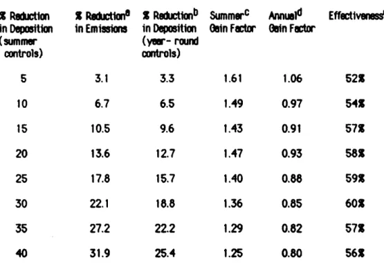
emission reduction remains the same regardless of whether substitution occured seasonally or year-round. Substituting a given quantity of gas for coal or oil will reduce emissions by some constant amount regardless of when during the year substitution occurs; the same is not true with respect to deposition. The annual deposition reduction is smaller in the case of year-round controls because the winter transfer coefficients are smaller. Table 6 presents the GF for each of several levels of seasonal and year-round gas substitution. For example, for a 25% reduction in deposition, there is a corresponding 3.9 million ton or 18% (if a 22 million ton base is assumed) reduction in S02 emissions, (due to 1176 bcf of natural gas being substituted for coal and oil). If this same quantity of gas were evenly substituted year-round, emissions would still be reduced by 18%, but, because both summer and winter transfer coefficients are used, the deposition reduction is now 16%. The GF for seasonal substitution is (25%/18%)-1.40, while that of year-round substitution is

(16%/18%)-0.88. Hence, seasonal substitution is 59% [(1.40%/0.88% )-1.591 more effective than year-round substitution at this level. Figure 8 is a graphical

effectiveness varies somewhat because the relative amount of gas substitution occuring in each state varies at different levels of deposition reduction.

The GFs for both seasonal and annual controls are diminished at higher levels of deposition reduction. This is because plants further from the receptor are included in the solution as the deposition reduction becomes larger. The distance between the two

lines in Figure 6 represents the superiority of seasonal over annual gas substitution.

This distance remains relatively stable regardless of the level of deposition reduction.

In general. a seasonal control strategy is 52-60% more effective than an annual control strategy for reducing deposition at an Adirondack recentor.

VI. 2. The Effect of Substitution on Fuel Consumption

Each plant in the model burns a known quantity of coal or oil annually (EIA, 1984a). It has been assumed that half this quantity is consumed during April through

September. This is supported by evidence that net generation by coal-fired plants

during April through September is 51% of annual net generation in the eastern 31

state region during 1983 (Figure 2).

When a plant is chosen by the model for gas substitution, the coal or oil it would burn during April through September is replaced by natural gas. The quantity of gas substituted is determined by calculating the quantity of gas that would be needed to

replace the btu output that the coal or oil would produce. The average heat content for

coal and oil at each plant is used for this calculation (EIA. 1984a).

For natural gas, a heat content of 1000 btu per cubic foot is assumed. Acutal average heat content for natural gas in the U.S. is approximately 1050 btu/cubic foot (EIA, 1984b); a 5% reduction to 1000 btu/cubic foot has been allowed to account for boiler derating. i.e. a 5% loss in boiler output. Basically, derating occurs because a boiler designed to burn coal or oil does not burn gas with equal effectiveness because of

differences in the combustion characteristics of the fuels. Experience with derating

due to gas substitution is meager, since gas substitution in coal and oil burners is very limited at present. Five percent is a reasonable allowance. based on experience with substituting natural gas for oil at Boston Edison's Mystic 7 unit (Boston Edison, 1985). Detailed work on dersting and inefficiencies caused by burning gas in boilers designed for coal or oil is left to future analyses.

The model calculates the quantities of gas substituted and coal and oil displaced for the various levels of deposition reduction that the model was exercised for, as shown in

the bottom half of Table 5. These quantities were mentioned earlier in the case of 20% and 30% deposition reductions. Figures 9, 10, and 11 show curves of these quantities.

Initially most of the gas is substituted for oil. However, because oil's contribution to deposition is very small, coal quickly becomes the object of substitution. To illustrate, Figure 11 shows that for a 5% deposition reduction, gas displaces 79 million out of a possible 97 million barrels of oil, i.e. 80%. For coal. Figure 10 shows that 8 million out of a possible 176 million tons, i.e. less than 5%, is displaced. For a 20%

deposition reduction, the respective percentages for oil and coal are 90% and 30%, oil's percentage rises only slightly while coal's percentage increases by a factor of six. Hence, beyond the lowest levels of deposition reduction, substituting gas for coal is nearlv,comnletelv resoQnsible for further reductions.

VI. 3. The Average Cost of Emission Reduction

Figure 12 shows the reductions in S02 emissions for various reductions in deposition. Using this and the total cost data, the average cost of emission reductions at various levels of deposition reduction can be calculated (Figure 13). The average cost of reducing S02 emissions via seasonal gas substitution ranes from a negative $340 nor ton S02 at the 5% denosition reduction level (from Figure 12 this corresponds to a 0.6 million ton reduction in emissions). to a ositive S1584 oer ton S02 at the 40% deposition reduciton level (a corresponding 6.9 million ton emission reduction). (The cost of emission reduction is negative when there is a negative price differential, i.e. when oil is more expensive per btu than natural gas). For comparison, the S02 removal cost by limestone flue gas desulfurization (scrubber) was reported to be in the range $576-1126 per ton (Miller, 1985). From the sixth column in Table 5, it can be seen that the average cost of seasonal gas substitution is in or below the average cost range for scrubbing, for up to a 25% reduction in total annual deposition at the Adirondack receptor. The conclusion is that there are a substantial number of plants where the cost of seasonal gas substitution is competitive with that of scrubbing.

As noted earlier, the costs of seasonal gas substitution are based on 1983 fuel price differentials. Future price differentials may vary, consequently, future costs may be

different,

VI. 4. The Average Cost of Deposition Reduction

on the expected costs of reducing S02 emissions. Total cost and S/ton of S02 removed are frequently used to compare alternative control strategies. In making these comparisons, a distinction should be made between receptor-oriented (or targeted) strategies that maximize the amount of deposition reduction at a receptor(s) for a unit of emission reduction, and source-oriented strategies aimed solely at reducing total emissions. A direct comparison of the cost of receptor- and source-oriented strategies

can be misleading; these strategies will not result in equal deposition reductions at a given receptor for equal emission reductions.

In order to facilitate a direct comparison, it is useful to define a cost per unit of deposition reduction at a particular receptor. Dividing the total cost for seasonal gas substitution by the corresponding quantity of deposition reduction at a receptor, produces a measure of the average cost of reducing deposition at that receptor. The average cost of deposition reduction at an Adirondack receptor, expressed in terms of billions of dollars per kg S04 per hectare per year (B$/kg S04 ha I_{yrl), is shown in} Table 5, column 4. The average cost for deposition reduction ranges from a negative $0.165 billion/ kt S04 hair-lt. for a 5% deposition reduction to $1.002 billion/ kt S04

hI;!-i

After first determining the resulting deposition reduction, the average cost of deposition reduction may be calculated for any source-oriented emission control strategy. Cost comparisons, based on the cost of deposition reduction rather than the cost of emission reduction, can then be made between seasonal gas substitution and source-oriented control strategies. The following section illustrates such a comparison.

Morrison and Rubin (1985) developed a model that computes the emission reduction and cost that would result from emission caps of 1.5 and 1.2 lbs. S02 per million btu on utility emissions using optimized combinations of switching to lower sulfur coal and flue gas desulfurization (FGD). The 1.5 and 1.2 lbs. emission caps resulted in annual emission reductions of 8 and 10 million tons S02 respectively. Based on the distribution of emission reductions across the eastern 31 states, these emission reductions would respectively yield 7.2 and 8.2 kg S04 ha 1 _{yfrt deposition reductions} at an Adirondack receptor (calculated using the MIT acid deposition model annual transfer coefficients). These quantities of deposition reduction are respectively equivalent to 26% and 30% reductions from the 27.5 kg S04 hal1 _{base deposition level} at an Adirondack receptor.

Table 7 summarizes the following comparisons. Morrison and Rubin calculated total cost ranges of $1.5-2.6 and 3.2-4.7 billion (1980S) for the S and 10 million tons of S02 emission reductions, respectively. Using a GNP deflator of 1.2 to adjust to 1983 dollars makes the cost ranges $1.8-3.1 and 3.8-5.6 billion, respectively. Dividing the cost by the deposition reductions gives $0.25-0.43 and 0.46-0.68 billion per kg S04 deposition removed, respectively, for the two cases. Referring to Table 5, column 4, the average cost of deposition reduction for similar (25% and 30%) reductions via seasonal gas substitution is $0.64 and 0.72 billion per kg. The conclusion is that, for 25% and 30% deposition reductions fat an Adirondack receptor, Morrison and Rubin's optimized straegy has a lower average cost per kilogram of S04 reduced than does seasonal gas substitution. This is not to my that seasonal gas substitution is not cost-competitive with other control strategies, in this case an optimized combination of switching to lower sulfur coal and FGD. I respectfully submit that Morrison and Rubin's is but one control strategy; other control strategies will have different costs, some higher and some lover. The purpose of the preceding comparison is primarily to show that cost comparisons with respect to deposition can be made between source-and receptor-oriented strategies.

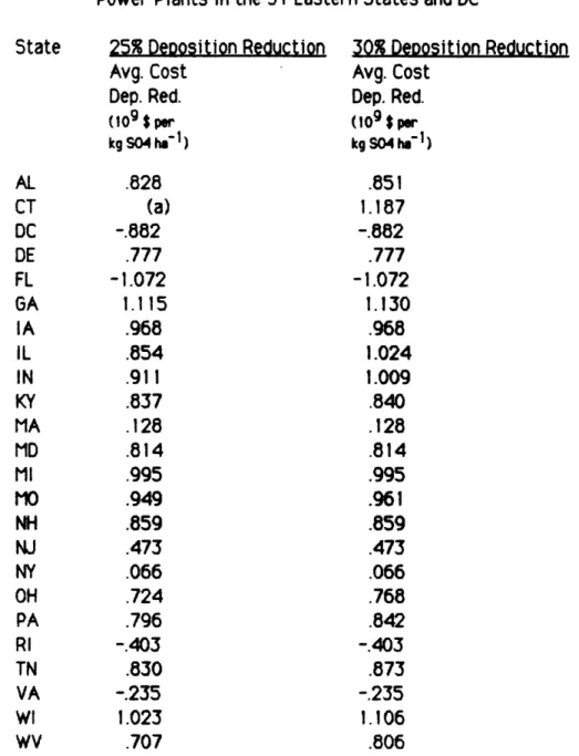
Using the data in Appendix C, state-level average costs were computed for 25% and 30% deposition reductions (Table 8). Figures 14 and 15 show this data ranked from lowest to highest, plotted against the cumulative percentage deposition reduction of the states. For example, in Figure 14. Ohio's (OH) average cost is $0.724 billion per kg S04 hal, at the 25% deposition reduction level; it accounts for an approximate 5% deposition reduction by itself, and together with preceding states accounts for a 12% deposition reduction.

While the average costs for seasonal gas substitution in the entire eastern 31 state region are higher than those derived from Morrison and Rubin's two cases for equivalent deposition reductions, there are several states that do have average costs of

achieving deposition reduction via seasonal gas substitution that are within the

ranges of Morrison and Rubin's cases. The following states, DC, FL, MA. NJ, NY, RI, and VA, have average costs that are in or below the ranges specified by Morrison and Rubin, namely $0.25-0.43 billion (25% reduction) and $0.46-0.68 billion (30% reduction) per kg S04 ha' 1 reduced. Thus, it appears that seasonal gas substitution may be cost-competitive with other control methods, in this case an optimized combination of switching to low-sulfur coal and FGD, in some states.

VII. GAS SUPPLY FOR SUBSTITUTION

The seasonal gas substitution model has not considered gas deliverability

constraints which may limit the amount of substitution that occurs within a state as

specified by the model. A gas deliverability constraint would occur whenever the gas supply infrastructure lacks the necessary capacity to meet the incremental demand imposed by a level of gas substitution, or if total gas production is exceeded by the incremental demand. In order to utilize gas substitution, the utility must access its gas supply from a gas distribution company's or gas transmission company's high-pressure pipeline. Tran ission capacity can be expanded, but this may increase fuel costs, which may make gas substitution les competitive relative to other control strategies.

Because the primary use of natural gas is for space heating, summer demand is

lower than winter demand in nearly all states. This condition favors seasonal gas substitution, but not in an unlimited or universal pattern. The ratio of summer sales volume to winter sales volume averaged 49% and ranged from 33% to 103% in the 31 eastern states and DC in 19B4 (Table 9). The winter/summer sales ratio is only an indicator of general capacity and cannot be relied upon as a derinitive measure of

excess capacity available to every generating unit within a state. For the purposes of this study it is assumed that the difference between winter and summer consumption

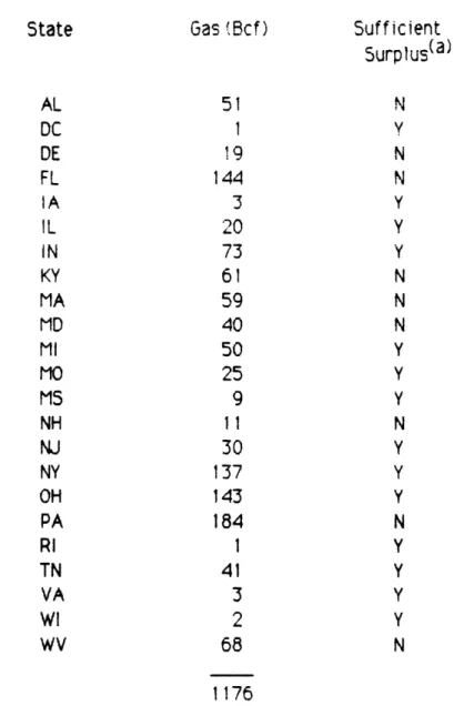
is an approximate measure of available capacity. The aggregate difference between summer and winter volume is 2030 billion cubic feet, which would provide approximately enough gas substitution for a 37% reduction in deposition (from Figure 7). However, not every state has the necessary surplus summer gas required at all levels of deposition reduction. For example, for a 25% deposition reduction, only 14 states have the surplus needed to supply their share of the model's solution. The summer surplus is estimated from Table 9. column 4; the incremental demand for gas

in each state sufficient for a 25% reduction in deposition is shown in Table 10.

While the availability of natural gas is a significant factor, as supply constraints

are not included in the model. This simplification is made because the availability of

gas is difficult to estimate within a state or at a given plant. The determination of

availability is left to those considering gas substitution. A general approximation of gas availability can be made by comparing seasonal sales volumes for selected gas transmission and distribution companies. Table lla shows the ratio of summer to

eastern US.; Table lb shovs the ratios for several gas distribution companies. It can be seen that excess summer capacity is generally available, but the amount varies greatly between companies and regions.

VIII. OTHER COSTS

Preliminary findings concerning incremental capital and operating costs for seasonal gas substitution reveal two significant points. First, capital costs are low and implementation is quick. Using as an example the Boston Edison Mystic *7 unit, an

oil-fired generating unit that converted to seasonal gas use, the boiler modification

and gas supply construction cost $3.5 million for the 565 MW unit and was completed in approximately one year (Boston Edison, 1965). This is approximately $6/kV. In contrast, capital costs for limestone flue gas desulftrization (scrubbing) are between $175 and $317/kW (Miller, 1983), and have much longer lead times. Second, ash

generation is reduced. If the variable component of ash disposal is significant, there

is a potential cost saving from seasonal gas substitution. For example, a 500 MV

coal-fired unit might produce 130,000 tons of bottom and flyash annually. If variable

disposal costs are $10/ton, the ash disposal cost is $1.3 million annually. Seasonal gas substitution could save one-half of this sum. The present value of these savings are

close to or may exceed the capital costs associated Vith seasonal gas substitution.

The crucial determinant of the cost-competitivenes of gas substitution is the price

differential between gas and coal and gas and oil. Since long term prices are impossible to predict with certainty. gas substitution is regarded as being financially risky when compared with other control methods. Actually, gas substitution my be les risky than more capital intensive control methods. Because there is relatively small capital investment associated with gas substitution, a utility could easily abandon it if a more cost-effective solution became available without forfeiting a large investment. Because of the large capital outlay needed for scrubbing equipment, a utility saddled with an expensive scrubber is financially limited if it wants to exploit less expensive control methods that may become available.

IX. CONCLUSIONS

Nearly all of the "acid rain" policy and policy analyses have focused on emission reductions and the cost of controlling emissions. But it is deposition, not emissions per

se, that matters. Monitoring has shown that deposition rates are significantly higher during April through September than during October through March for equal

emission rates. Based on this evidence, it is more efficient to control emissions (and

hence deposition) during the summer half of the year.

Seasonal substitution of gas for coal or oil is a reasonable option for utilities to control S02 emissions and is vwell suited to comply with policies which focus on controlling deposition. However, it is not a panacea for reducing S02 emissions. The quantities of gas needed for substitution in order to make total emission reductions of more that a few million tons per year in S02 emissions would exceed existing capacity in many states. Some generating units are located too far from a gas supply or face fuel cost differentials that are too large to make gas substitution economically competitive with other control methods. On the other hand, many generating units do have access to sufficient quantities of gas at costs that make gas substitution competitive with other emission control methods.

The cost-effectiveness of any control method should be related to its effect on deposition rather than its effect on emissions. One ton of S02 removed in the summer

half of the year has a greater effect on deposition than reducing that ton year-round. It was shown that in terms of equal deposition reductions in the Adirondacks. that the

costs of seasonal gas substitution and some year-round controls may be comparable in some states.

Conclusions:

* In some states seasonal gas substitution may be economically competitive with other control methods for achieving equal annual deposition reductions in sensitive areas.

* In some states gas deliverability and supply may limit the amount of gas substituted.