Control of heat conduction in manufacturing processes : a distributed parameter systems approach

Control of Heat Conduction in Manufacturing Processes:

A Distributed Parameter Systems Approach

by

Upendra V. Ummethala

Bachelor of Technology in Mechanical Engineering Indian Institute of Technology, Madras (1990) Master of Science in Mechanical Engineering University of California, Los Angeles (1992)

SUBMITTED TO THE DEPARTMENT OF MECHANICAL ENGINEERING IN PARTIAL FULFILLMENT OF

THE REQUIREMENTS FOR THE DEGREE OF

DOCTOR OF PHILOSOPHY at the

MASSACHUSETTS INSTITUTE OF TECHNOLOGY

June, 1997

@ Massachusetts Institute of Technology 1997

Signature of Author

Certified by

Department of Mechanical Engineering June 1997 Z UA David E. Hardt Thesis Supervisor Accepted by Ain A. Sonin Department of Mechanical Engineering Chairman, Department Graduate Committee

Control of Heat Conduction in Manufacturing Processes: A Distributed

Parameter Systems Approach

by

Upendra V. Ummethala

Submitted to the Department of Mechanical Engineering on May 8th_{, 1997 in partial fulfillment of the requirements}

for the Degree of Doctor of Philosophy in Mechanical Engineering.

Abstract

There are several manufacturing processes where heat conduction is one of the key physical phenomena that influence the process performance. Such processes include molding operations, heat treatment, welding, flame bending etc. Typical temperature control implemented in these processes, at best involves independent multi-zone type regulation. (For example: barrel heaters in injection molding.) This thesis has addressed the problem of controlling entire temperature distributions in such processes. Several techniques developed in the theoretical literature on the control of distributed parameter systems (DPS) have been investigated for their applicability to manufacturing processes.

An experiment has been setup using a scanned TIG torch to heat a rectangular specimen with several thermocouples embedded within it. A detailed simulation study was

performed on a model of this experimental setup, to study the closed loop behavior of the model under different scenarios. The simulations used a linear quadratic gaussian (LQG) controller. The conclusion from this study was that the distribution of inputs and sensors

in the controlled object had a significant impact on the performance of the controller in rejecting disturbances. However, there are no available techniques in the theoretical

literature to adequately address the issue of optimally distributing inputs.

This motivated the development of a technique for optimally distributing inputs across a controlled object. The technique comprises separating the space and time part of the governing partial differential equation, which results in the steady-state equation for heat conduction within the controlled object. The steady-state Green's function corresponding to this steady state heat conduction equation is determined. A quadratic performance index comprising a heat flux term and a temperature error term is defined over the spatial domain. A general form of a higher order cost functional is used along with the Green's function to set up the optimization problem. Variational calculus is used to determine the optimal heat flux distribution in steady state. This optimal heat flux distribution is in a linear proportional feedback form wherein the heat flux needed in steady state depends on the steady-state temperature error. Therefore such an approach can better adapt to model errors and external disturbances.

Simulations have been performed on a rectangular solid to illustrate the optimal distribution technique based on the steady-state optimization. The constraints on the locations of the inputs and the types of disturbances considered were selected based on typical requirements in a resin transfer molding (RTM) or a compression molding

application. The Green's functions were derived using a finite difference formulation for the heat conduction in the solid. The design of the heating was separated into two parts: In the first part, the heat flux locations and strengths were selected to satisfy the

requirements on the steady-state performance. In the second part, additional heaters were introduced to improve the transient performance. In the first part of the design, the high gain (MIMO) obtained as a part of the steady-state analysis was rolled off using a first order frequency blending function. The MIMO Nyquist criterion was then used to determine if the closed loop system was stable. The break frequency for the frequency blending function is used as a controller design parameter and a suitable value is selected. The predictions of the MIMO Nyquist criterion have been verified by simulating the closed loop system. Additional heaters placed closed to the surface have been

incorporated into the design using a cross-over network type design. The improvement in the transient performance has been demonstrated.

The problem of accelerated cooling of hot-rolled steel has been addressed as a transient temperature distribution control problem. The major source of disturbance in this process is a variation in the initial temperature of steel. There are no measurements possible once the cooling process begins. The anomalous nature of the cooling process amplifies the variations in the initial temperature distribution, if not compensated for. To compensate for the variations in the initial conditions, a finite horizon quadratic performance index is setup. The resulting feedback form for the optimal solution is simulated on the model for the process, with the initial condition varied from the nominal initial condition. The

simulated input is then used as an open-loop input to the process to compensate for the variations in the initial condition.

Thesis Supervisor: Prof. David E. Hardt.

Title: Professor of Mechanical Engineering, Massachusetts Institute of Technology.

Committee:

Prof. David E. Hardt (Chairman) Department of Mechanical Engineering MIT.

Prof. Jung Hoon Chun Department of Mechanical Engineering MIT.

Prof. Harris Doumanidis Department of Mechanical Engineering Tufts University.

Dr. Kenneth W. Kaiser Charles Stark Draper Laboratory. Dr. Herschell B. Smartt Idaho National Engineering Laboratory.

Acknowledgements

I would like to thank my advisor Prof. David Hardt for his guidance and support

throughout my thesis, working with Dave has been an invaluable learning experience. I would also like to thank the other members of my committee: Prof. Jung Hoon Chun, Prof. Harris Doumanidis, Dr. Kenneth Kaiser and Dr. Herschell Smartt for their invaluable comments and criticism. I would especially like to thank Dr. Kaiser for

spending many hours discussing and verifying the work on optimal input distribution. Also, I would like to say a special thanks to Prof. Doumanidis for letting me use his laboratory facilities. I would also like to thank the U.S. Department of Energy for

supporting this research.

Fred Cote in the machine shop has helped me with the machining for the experimental setups and I would like to thank him for his patience and help. I would also like to acknowledge the help that Nikos provided.

My parents and my wife have been extremely supportive during my thesis and I would like to thank them for their support. I would also like to thank all my friends who have made my stay at MIT rich with fond memories.

Upendra Ummethala June 1997.

r~ie

Table of Contents

CH APTER 1 ... 10

MOTIVATION AND BACKGROUND FOR TEMPERATURE CONTROL IN MANUFACTURING PR O C E SSE S ... ... ... ... 10

1.1. IN TRO D U C TIO N : ... 10

1.2 PROCESSES WITH HEAT CONDUCTION: ... ... 12

1.2.1. H eat treatm ent. ... 12

1.2.2. Injection M olding: ... 14

1.2.3. Compression Molding and Resin Transfer Molding (RTM): ... ... 15

1.2.4. W elding:... ... ... ... 16

1.2.5. Flam e bending: ... 19

1.2.6. The requirements on the processes: ... 19

1.3. DISTRIBUTED PARAMETER SYSTEMS (DPS) LITERATURE: ... 20

1.3.1. Publications on controllability, observability and stability:...20

1.3.2. Publications on optimal control and optimal sensor and actuator location: ... 21

1.3.3. Applications of D PS techniques: ... 24

1.3.4. Conclusions from literature survey:...24

1.4. M ODEL FORM S: ... 25

1.4.1. Eigen function expansion based models ... ... 26

1.4.2. Models Based on Spatial discretization:... ... 29

1.4.3 G reen's Function based m odels: ... 32

1.5 COST FUNCTIONALS: ... 34

1.6. STRUCTURE OF THE THESIS: ... 37

CH APTER 2 ... ... 42

STEADY STATE OPTIMAL CONTROL OF TEMPERATURE IN TWO DIMENSIONS ... 42

2.1 PRIOR EXPERIMENTS...42

2.1.1. The need for a detailed study to identify deficiencies in the state-of-the-art: ... 44

2.2 DESCRIPTION OF THE EXPERIMENTAL SETUP: ... ... 46

2.2.1. Idea behind the experiment: ... 47

2.2.2. Description of the hardware used for experiment: ... ... 52

2.3. MODEL FOR CONTROL: ... 52

2.3.1. Computation of the eigen functions and the eigen values: ... .... 55

2.3.2. Derivation of the State-Space model: ... 57

2.4. THE CONTROLLER DESIGN: ... 59

2.5. SIMULATION RESULTS...65

2.5.1. Effect of sensor location on controller performance: ... 66

2.5.2. Effect of input location on controller performance: ... ... 67

2.6. C O N CLU SIO N S: ... 79

CH APTER 3 ... 83

OPTIMAL INPUT DISTRIBUTION... 83

3.1 MOTIVATION FOR THE DISTRIBUTION PROBLEM ... ... 83

3.2 SPECIFIC TEMPERATURE CONTROL REQUIREMENTS ON DIFFERENT PROCESSES: ... 85

3.2.1 M olding Applications: ... 86

3.2.2 H eat treatm ent: ... 87

3.2.3. F lam e bending: ...89

3.2.4 D im ension control: ... 90

3.3 SUMMARY OF REQUIREMENTS FOR INPUT DISTRIBUTION: ... 92

3.4 DEFINING AN APPROACH FOR THE PROBLEM: ... ... 92

3.4.1. The method for input distribution and controller design:... ... ... 94

3.5 M ODEL DEVELOPMENT: ... ... 94

3.6 COST FUNCTIONALS ... 99

3.6.1. Example cost functionals: ... 100

3.6.2. Generalized form of cost functionals:... ... 102

3.7 DERIVATION OF THE CONDITION OF OPTIMALITY: ... 103

3.8 EXAM PLE PROBLEM S: ... ... 106

3.8.1. Exam p le 1:.... ... 107

3.8.2. Example 2: ... . ... 110

3.8.3. Example 3: ... 111

3.9. DESIGN PROCEDURE FOR SPECIFIC PROCESSES:...12

3.10. CHAPTER CONCLUSIONS: ... 114

CH A PTER 4 ... 116

OPTIMAL DESIGN OF HEATING AND COOLING: AN EXAMPLE ... 116

4.1 INTRODUCTION :...116

4.1.1. Resin Transfer Mold (RTM) example problem: ... 118

4.2 SIM ULATION SET-UP: ... ... 119

4.3 FINITE DIFFERENCE MODEL FOR DERIVING INFLUENCE FUNCTIONS:... ... 121

4.4 THE OPTIMIZATION OVER SPACE: ... 126

4.4.1. Effects of model errors: ... 128

4.4.2. Design procedure for narrowing down the locations of input:... 129

4.6 DESIGN PROCESS FOR SELECTING LOCATIONS FOR HEAT FLUX: ... 136

4.6.1. Input restriction to half of the mold: ... 136

4.6.2. Effect of disturbances on closed loop behavior: ... 137

4.6.3. Input restriction to fewer locations:...147

4.7 CONCLUSIONS FROM STEADY-STATE DESIGN: ... 159

4.8 T RANSIENT D ESIGN : ... ... 159

4.8.1. The D ynam ic m odel: ... 161

4.9. ROLLING OFF THE GAIN TO STABILIZE THE SYSTEM. ... 165

4.10. VERIFICATION OF THE MIMO NYQUIST PREDICTION: ... 171

4.11. IMPROVING THE RESPONSE OF THE SYSTEM WITH ADDITIONAL HEATERS: ... 178

4.12. CONCLUSIONS: ... 183

CH APTER 5 ... ... 187

OPTIMAL CONTROL OF TRANSIENT TEMPERATURES: EXAMPLE... 187

5 .1. IN TRO D U CTIO N ... 187

5.2. REQUIREMENTS ON THIS PROCESS: ... ... 191

5.3. SOURCES OF DISTURBANCES: ... ... ... ... 193

5.4. ANOMALOUS NATURE OF THE COOLING WATER JETS: ... 194

5.5. M ODEL FOR PROCESS: ... 200

5.5.1. Finite difference based model for the heat conduction in the slab: ... 201

5.6. CONTROL APPROACH: ... 204

5.6.1. Process requirements... ... ... 204

5.6.2. Optimal closed loop solution:... 204

5.6.3. Optimal open-loop solution: ... 207

5.7. NUMERICAL SIMULATION OF THE COOLING PROCESS ... 209

5.7.1. Details of simulation set up: ... 209

5.7.2. Numerical techniques for computing optimal solution: ... ... 211

5.7.3. Selection of parameters in cost functional:... ... 212

5.7.4. Simulation results ... ... ... 213

5.7.5. Control method when material properties have temperature dependence:...215

5.8. CONCLUSIONS: ... 216

CHAPTER 6 ... 221

CONCLUSIONS AND FUTURE WORK ... 221

6.1 CONCLUSIONS FROM THESIS: ... 221

6.2 FUTURE WORK: ... 223

6.2.1. Optimal sensor location in heat conduction systems:... ... 223

6.2.2. The optimization method: ... 225

6.2.3. Experimental setup for studying optimal sensor location:... ... 226

6.2.4. O ther Future work: ... 227

Chapter 1

MOTIVATION AND BACKGROUND FOR TEMPERATURE CONTROL IN MANUFACTURING PROCESSES

1. 1. Introduction:

In many manufacturing processes, temperature fields and heat fluxes are the primary determinants of the process output and product quality. Such processes include all

solidification processes (casting, molding, welding) as well as solid phase processes

where thermal cycles are used to change properties or shape (e.g. heat treating and line

heating). A few such processes are discussed in section 1.2.

Influencing the process outputs such as material, geometric and mechanical properties in

all such processes, involves controlling the temperatures and heat fluxes. The processes considered in this thesis involve situations where heat conduction is the dominant

physical phenomenon in determining the temperature distributions. This means that the

temperature distributions and heat fluxes are governed by the heat diffusion equation. Equation 1.1.1., shows the heat diffusion equation:

dT

pC, (-,t) = V(k(T)V)T(x,t) + (x, t); 1.1.1 Bo(T(, t)) = 0; Boundary Condition

p: is the density

V = +

d

+

C,: is the specificheat d dz

k(i): is the conductivity of the material Bo: Boundary conditions 1.1.2

x: is the vector spatial coordinates T(i, t) : temperature distribution

t :is time _{O((x, t) : distribution of the heat flux}

The heat flux O(x, t) , which is incident on the solid within which the temperature is

being controlled, comprises of two components (see equation 1.2.3.). The first

component is the heat flux that can be actively manipulated and it will be referred to as

the controller heat flux c (i,t). The second component of the total heat flux, which

cannot be actively manipulated, is referred to as the disturbance heat flux D (x , t).

((X, t) = Oc(X, t) + D (X, t) 1.2.3. For example, consider the problem of controlling the temperature distribution in an injection mold, using cartridge heaters and cooling oil, when ambient temperature

changes during operation. The heat flux generated by cartridge heaters and cooling

passages can be actively controlled and hence any heat flux input due to these devices

will be considered to be the controller heat flux. However, the heat flux experienced by the mold due to changes in the ambient temperature would be a part of the disturbance heat flux.

Section 1.2 discusses some example processes where temperature control is of importance. These are the processes that have motivated this thesis.

1.2 Processes with heat conduction:

Manufacturing processes are characterized by phenomena that have a spatial and temporal variation. In the processes being studied here, heat conduction which is a spatially

distributed phenomenon, determines the process outputs. In some such processes, simple

lumped parameter models that do not capture the distributed nature of the heat conduction

phenomenon are used. These may be adequate in the manufacture of components where

the requirements on the process are not demanding. However, with more stringent

quality, productivity and energy consumption requirements on the processes, one needs to fully consider the spatially distributed nature of the heat conduction in these processes.

This will lead to techniques that better aid in designing systems for heating and cooling

and thereby improving process quality, productivity and energy consumption.

1.2.1. Heat treatment.

Several products are manufactured by varying the temperature trajectory through which the material of the product is taken through. Most steel products such as sheet steel,

beams for construction, steel slabs for bridges and pressure vessels are subjected to

different types of heat treatment. The specific temperature trajectory for each product is

dependent on the microstructure desired at different locations in the product. See

Kalpakjian(1995) for some examples of heat-treatment operations and corresponding desired temperature trajectories.

Figure 1.2.1. shows a schematic of a steel slab being cooled using jets of water. The edges have to be warmed with induction heaters to ensure the uniformity of temperature across the slab.

COOLING SPRAY

INDUCTION HEATER

Figure 1.2.1. A cross-sectional schematic of the heat treatment operation for steel slabs.

The goal in this process is to take the material through a desired temperature trajectory T(x,y,z,t). The temperatures experienced at different locations determine the material

properties at different locations within the slab being produced. By modulating the

cooling sprays and the induction heaters at different locations, the temperature distribution throughout the slab can be manipulated.

This control has to be implemented such that the total amount of water consumed is within acceptable limits. Simultaneously one has to ensure that the temperature

distribution trajectory achieved should be within acceptable limits in the presence of process disturbances. The benefits of using such controlled cooling will be discussed in

detail in Chapter 5., which details the specifics of the method for controlling transient

temperature distributions.

1.2.2. Injection Molding:

The mold temperature is one of the determining factors in the quality and consistency of a

product produced using injection molding. There are several disturbances on the process

that include: change in the ambient temperature, change in the temperature of the plastic,

changes in the performance of the cartridge heaters or cooling oil of the mold, gradual heating and cooling of the mold due to coming in contact with the plastic etc.

Sometimes it is desirable to impose gradients across the mold. (See Jansen(1993) for

example). The residual stress state in the part being produced using injection molding, is

dependent on the coupling between the pressure and the temperature profiles of the cooling plastic. By carefully controlling the temperature profile, one can ensure that parts

with desirable residual stress states are produced. Jansen(1993) and Sha(1995) have done

some preliminary studies on the effect of temperature variations on the stress-state and

distortions on a part produced by injection molding. These studies have shown

qualitatively, that changes in mold temperature distributions do effect the residual stress state and the optical properties of objects being produced. However, in order to conduct

better experimental studies, efficient mold temperature control is needed.

The temperature distribution within the mold is dependent on the locations of the heating

and cooling. Similarly, locations of the thermocouples determine the efficiency with which disturbances are detected. The ability of any controller to efficiently compensate

for the disturbances occurring is also dependent on the locations of heating and cooling.

Chapter 4., shows a technique for designing locations of heating and cooling in order to

accurately control the temperatures in a mold.

1.2.3. Compression Molding and Resin Transfer Molding (RTM):

Compression molding and RTM are processes used for manufacturing composite parts

for different applications. Both these processes are matched die processes, which involve

taking the composite part through a specified temperature trajectory. Typically the part is heated so that the temperature everywhere is uniform. The heating causes an exothermic

reaction in the resin within the part and causes it to cure. The disturbances in this process

include all of the disturbances one would deal with in the case of injection molding and in

addition, the uncertainty in the exothermic reaction manifests itself as an additional

disturbance. Figure 1.2.2. shows a schematic of a typical mold with heating and cooling in it.

The controller design needs to be performed so that the steady-state temperature error is minimized while ensuring a stable operation for the closed loop system. At the same time

one needs to minimize the number of heaters and cooling passages that one uses to control the process. The best location for a given set of heaters and coolers needs to be found.

In Chapter 4., presents an approach for designing the distribution of heating and cooling in such a mold so as to maintain a desired temperature distribution on the mold surface.

1.2.4. Welding:

In a welding process, an intense heat source such as an electric arc or a laser is moved

over the surface of the component being welded. Filler material is sometimes added. The nature of heat transfer in a traditional welding process, causes a heat effected zone (HAZ)

around the weld. In addition, the geometric attributes of the weld such as the width W of

the weld and the depth D of the weld are dependent on the temperature trajectory that the

base material goes through. See Doumanidis (1988) and Masmoudi (1993). The process outputs such as the depth of weld, HAZ etc. are highly coupled and it is very difficult to

independently control these attributes The welding process could be better controlled

using a flexible heat source got by scanning a heat source such as a welding torch.

Doumanidis (1996) has recently implemented such a control for a scan welding process.

The goal of the controller in this process is to be able to achieve a certain specified

characteristics for the weld. However, approaching this problem via distributed parameter systems could yield insight into the best achievable performance given the

RWTh-Orpi

W

c

Cmrpote pat

Heaem

7

ompres

mdd

Cooling Passages

Welding torch

W_

Jeld

Bead

Figure 1.2.3. Geometry of the weld in a typical welding process.

/

Thermal Gradients

Figure 1.2.4. Flame bending or tool-less forming 11A7

I"ML

1.2.5. Flame bending:

Flame bending is a process used to manufacture one of a kind plates with specific

curvature. Flame bending is also termed as tool-less forming. A heat source such as a

flame or a plasma torch is scanned along specific lines in the component to induce

thermal stresses in the component. The thermal stresses cause permanent distortions in

the plate being deformed.

This process is employed to bend large and thick components in very low volume

production. The components produced by this method are typically used in ship building

and the manufacture of pressure vessels. Additionally, this approach could be used to

rectify the errors induced by other methods of forming.

The current industrial practice of flame bending involves bending the parts using a trial

and error method where incremental amount of bending is induced at each pass of the

flame. However, by better controlling the temperature distribution in this process better control over the distortions could be obtained.

1.2.6. The requirements on the processes:

In all of the processes discussed in this section, there is a need for controlling temperature distributions. The specific requirements may vary from process to process. In some

instances, one is interested in controlling the steady-state temperature distribution.

(Example: Mold temperature control). In other instances one needs to control a time trajectory of the temperature distribution. (Example: Heat treatment). In examples such as distortion control and length control one needs to control either the gradient of the

temperature or an integral of the temperature. One of the common requirements among

all the processes is that one needs to minimize the amount of hardware (e.g., heaters,

torches, thermocouples etc.) and the amount of energy used. This has to be done while

guaranteeing the performance of the process. The control theory that is of relevance to

present applications is in the field of distributed parameter systems (DPS) theory. The DPS theory is concerned with controlling phenomena that are distributed in space and

vary with time. The problem of controlling heat conduction/ diffusion equations has been

widely studied in the distributed parameter systems literature. In the following sections a

review of the literature in the control of Distributed Parameter Systems (DPS) is

presented.

1.3. Distributed Parameter Systems (DPS) Literature:

There is a good deal of published research on the topic of controlling distributed

parameter systems. The theoretical aspects of controlling such systems have been addressed, among others, by: Lions, (1971,1980), Balakrishnan, (1965,1976),

Butkovskii, (1969,1987), Delfour (1972,1982), Fattorini (1967,1985), Mitter (1969), Russell (1973), Wang, (1964) Vidyasagar (1973). Several books and collections of

papers have been published on this topic: Butkovskii (1969,1987), Omatu and

Sienfeld(1983), Ray and Lainiotis (1978), Aziz, Wingate and Balas (1977), El Jai and Pritchard (1988), Tzafestas (1982) etc.

1.3.1. Publications on controllability, observability and stability:

There is a plethora of publications dealing with system theoretic concepts such as controllability, observability and stability of distributed parameter systems.

Controllability of the heat conduction system has been studied by several authors, for

example: Omatu and Seinfeld (1989), Tzafestas (1978), Amouroux (1975,78), Goodson

and Klein (1970), Sakawa (1974), Butkovskii (1969), Russell (1973), Fattorini (1967), Seidman (1973) , Kamen (1976), Lions (1980), Triggiani (1975), etc. The range of publications is varied. While Omatu and Seinfeld (1989), Tzafestas (1978) etc. have

studied the controllability problem using eigen function expansions, authors such as Lions (1980), Triggiani (1975), etc. have addressed the problem using function theoretic

concepts.

Observability for DPS was defined by Wang(1964). Goodson and Klien (1970) have

derived observability results using an eigen-function expansion and this approach for

checking for observability can be found in a wide variety of publications. See: Omatu

and Seinfeld (1989) for a detailed derivation of several observability results.

Publications dealing with stability issues are far fewer and are very situation specific. Wang, (1964b, 1971) show a couple of publications with stability results for specific

diffusion systems with delays.

1.3.2. Publications on optimal control and optimal sensor and actuator location:

For manufacturing applications, optimal control and optimal sensor and actuator location are by far the most important issues to be considered. Butkovskii (1969), Goldwyn, Sriram and Graham (1967) present a technique for time optimal control of heat

conduction systems. Amouroux and Babary (1978) discuss optimal control with point

systems with mobile actuators. Ahmed and Teo (1981) has a collection of papers dealing

with Optimal control of DPS. Bellman (1957) and Lions (1971) treat the theoretical

aspects of the problem of optimal control of DPS. Lausterer (1977) discusses an example

of optimal control of a steel billet using LQG techniques. Kaiser (1968) discusses an

optimal control approach that addresses the problem of steady-state optimal control of temperatures.

The problem of optimal location of actuators and sensors is unique to distributed

parameter systems. The performance of any controller depends critically on the location

of the sensors and actuators. This problem has been widely studied in the literature. El

Jai and Pritchard (1988) and Kubrusly and Malebranche (1985) have exhaustive surveys on this topic. Sensor location literature primarily deals with locating point sensors,

however there are no guidelines for locating sensors that might have a distribution to them. For example: if one could scan a pyrometer along specific lines to estimate

temperatures, there are no guidelines on how to select the lines along which the pyrometer measurements should be scanned on. Kaiser (1971) illustrates one way of

optimally distributing sensing for a steady-state one-dimensional length control problem.

Most of the sensor location publications deal with minimizing some measure of steady-state error covariance of an optimal estimator such as a Kalman Filter. Some algorithms involve, sequentially locating the sensors, minimizing the error covariance at each step.

Other algorithms attempt to simultaneously locate N sensors so as to minimize the error covariance of the optimal estimate. Bensoussan (1972) showed the existence of solution for the optimal location problem using the covariance of the optimal estimate. Yu and

Seinfeld (1973) first developed a sub-optimal method of sequentially locating sensors. Most algorithms used to evaluate the optimal locations involve some form of numerical

optimization and are very numerically intensive, even for problems with simple

geometries.

Amouroux and Babary (1975,78) discuss optimal location of actuators where the

locations of the actuators are selected so that a quadratic performance index similar to t e

cost in a linear quadratic regulator problem is minimized. Omatu and Seinfeld (1983)

illustrate a technique for optimal location of both point actuators and point sensors,

simultaneously. This technique involves minimizing the performance criterion on the LQG problem. Kaiser (1971) illustrates a technique for determining optimal

sensor-actuator location and distribution for controlling steady-state temperature distributions.

El Jai and Pritchard (1988), Amouroux and Babary (1979) have addressed the problem of

determining optimal shapes or domain of action (regions within the controlled solid where the input acts) for inputs. These publications deal with extremely simple

geometries and simple shapes for domains of action. The problems are numerically

solved after posing a parametric optimization problem. The applicability of these techniques is in doubt due to the several simplifying assumptions made. A technique

developed by Kaiser (1969) which uses a 'Greens function' based description for the he t conduction process, can be efficiently applied to problems dealing with steady-state temperature control. The approach presented by Kaiser, involves minimizing a quadrati/

flux. The optimal heat flux distribution thus obtained is in a feed-back form wherein the heat flux depends on the temperature error. This implies that the heat flux distribution s

dependent on the disturbances and model errors and therefore a better scheme from an application point of view. This thesis builds on the techniques developed by Kaiser

(1969).

1.3.3. Applications of DPS techniques:

The applications and experimental implementations to the DPS theory have been very few. Lausterer (1977), Morari and O'Dowd (1980), Mader(1976), Kaiser (1968) have

performed experiments on controlling temperature distributions. All of these experiments involved control of steady state temperature distributions. In Lausterer and Ray (1977)

the heaters and thermocouples were placed at arbitrary locations in the solid and a

sub-optimal state estimator has been implemented. The purpose of the experiment was to verify the performance of the theoretical results in DPS estimation rather than to facilitate

better control in any specific process. Kaiser (1968) demonstrated temperature control in

a rod for controlling the length in the presence of thermal disturbances. All the other

applications involve experimental setups used to verify theoretical results as opposed to

real applications.

1.3.4. Conclusions from literature survey:

In spite of the vast amount of theoretical and experimental research on the control of distributed parameter systems (DPS), there are virtually no real industrial applications o DPS theory to manufacturing processes. The reasons for this could be many. One of th

f

require a large amount of computing power. With computing power becoming cheaper,

these methods will be more attractive to implement. Additionally, quality, productivity and flexibility issues in manufacturing processes are becoming increasingly important.

Environmental requirements on processes have put energy conservation requirements o

the processes. Hence, the investigation of more advanced control methodologies, which might yield better performance of the manufacturing processes, has to be performed.

In the following section, model forms used in implementing DPS controllers will be

discussed.

1.4. Model forms:

Equations 1.1.1. and 1.1.2. show the governing equation for linear conduction of heat.

For control and analysis purposes, this equation needs to be modified into forms that are more suited to applying different control techniques. There are three major approaches

for performing this:

1. The first approach involves the use of the eigen function expansion of the partial

differential equation (PDE) in equation 1.1.1. and 1.1.2. The PDE can be equivalently

represented using an infinite set of ordinary differential equations that are derived using the orthogonality property of the eigen functions. The infinite set of equations

is then truncated to get a finite dimensional approximation to the PDE. This approach is by far the most common approach seen in most of the distributed parameter

2. The second approach uses some form of spatial discretization such as a finite

difference equations (FDE) based scheme. This involves spatially lumping the

geometry and deriving governing ordinary differential equations by performing energy balance between neighboring nodes. Finite element and boundary element

approaches are also based on spatially discretizing the solid, similar to FDE. These

methods are widely employed in the analysis of thermal systems.

3. The third approach utilizes an integral equation representation for the temperature

distribution using Green's functions. The Green's function can be experimentally

determined, hence this is a useful technique.

These three approaches have been used in this thesis for different problems. In this

section a brief description of each of the techniques is presented along with the pros and

cons of each approach.

1.4.1. Eigen function expansion based models

The eigen-function expansion based approach involves computing the eigen values and

eigen functions associated with equation 1.1.1. Say the eigen functions and eigen values

associated with equation 1.1.1. are:

D i(T) : Eigen functions i = 1,2,...,oo •t

: Eigen values 1.4.1.

Where i is a vector of spatial coordinates used in the problem. For the heat conduction system, the eigen values are all negative and decreasing and the eigen functions form a complete set. This implies that any piece-wise continuous function can be represented as a weighted infinite sum of the eigen functions. ( See Courant and Hilbert (1962)). The

temperature within a solid is a continuous function, hence the temperature can be written as an infinite sum of the eigen functions as:

00

T(i,t) =

X

i=1

Where:

x: Vector of coordinates

t: time

T(i, t) : Time varying temperature distribution in

the solid

ai (t) : Fourier coefficients corresponding to the ith eigen function D i(i)

Based on this eigen-function expansion a state-space representation can be derived by

substituting equation 1.4.2 in 1.1.1. (See Kubrusly and Malebrance (1985) for a detailed

derivation of the state-space equations). Additionally, chapter 2., presents a detailed example of using an eigen-function expansion to derive a state-space description to the

heat conduction problem. In the eigen function expansion based model, the Fourier

coefficients ai(t)'s are the states and the corresponding state-space model is given in

equations 1.4.3-1.4.8.

X= AX+BU 1.4.3.

Y = CX

Where the state vector and the initial value of the state are given by:

X(t) = [a1 (t),a2 (t),- ..]T

1.4.4.

X(O) = [a1 (0), a2 (0),...]T

Axn =diag -y=, }, n= 1,2,3,- --oo 1.4.5.

k

where ' - is the diffusivity.

pC,

If the heat flux distribution can be separated into its space and time parts, it can be written as shown in equation 1.4.6.:

O(X,

Where Q(i) is the vector of functions describing the distribution of the inputs and U(t) is

the vector of intensities of each of the inputs. This separation is only possible in situations where the locations where heat flux is applied is fixed in time, for example:

heaters and cooling passages whose locations do not change with time. The length of tie

Q(x) vector is dependent on the number of independent inputs that are available in the

process. The time varying amplitude of each of the inputs is governed by the values of

each entry in U(t). This decoupling is not possible in situations where the heat input devices are moving, for example: heating with moving torches etc.

In situations where the space and time parts can be decoupled, the B matrix of equation 1.4.3. is given by: (See Kubrusly and Malebrance (1985))

Bi = fffci(3)Qj(x)dV i= 1,2,---oo; j=1,2,---p D

p :Number of inputs 1.47.

D :Whole spatial domain spanning the solid

Similarly, if thermocouples in fixed locations are used to measure temperatures, the C matrix can be computed as:

Cj = f j()8(- -i)dV i = 1,2,...q j = 1,2,...oo 1.4.8.

D

Where 3(x - X-) is Kroneker delta with T~'s the locations of the q thermocouples.

This eigen function based model is truncated at a suitable dimension to give a finite

dimensional approximation to the infinite-dimensional system. In most applications the physical input devices (heaters and coolers) do not have a high spatial frequency content,

hence it is very difficult to "excite" the higher spatial harmonics. The eigen function

based models are, therefore, tend to be of a lower order.

The main disadvantages of using eigen function based models are:

1. The eigen functions are very sensitive to parameter variations and changes in boundary conditions.

2. For complicated geometries they are more difficult to evaluate. Most standard Finite

Difference Equations (FDE) and Finite Element Analysis (FEA) packages do not have

the ability to extract eigen functions and eigen values for the heat diffusion problem.

3. They cannot be experimentally computed.

4. The effects of non-linearities and model uncertainties cannot be easily studied.

1.4.2.

Models Based on Spatial discretization:

Modeling techniques such as finite differences and finite elements, involve discretizing the domain into smaller parts and applying energy conservation to each element to

determine the interaction between successive elements. For example the rectangular solid

temperatures at different nodes, in this finite difference grid is shown in figure 1.4.2.

Using this discretization, the governing equation for the temperature at the ijth _{node can} be written by performing energy balance at that node. Equation 1.4.9., shows the resulting equation:

dT

-1.4.9.

+ kT-2 [ _{j+ Tij-1 - 2Ti'j + qi,j}

(Ay)

In equation 1.4.9., qij _{is the external heat input or the internal heat generated at the} ijth

node, p is the density of the solid, C, is the specific heat of the solid and k is the thermal

conductivity. Ax and Ay are the dimensions of the finite difference grid as shown in

figure 1.4.2.

Equations similar to 1.4.9. can be written for all the nodes in the solid and arranged in a

vector to create the matrix differential equation:

S= AX + BU;

X [T,,T2...,mn ]T;

U = [q, q2"... qmn ]; _1.4.10.

m :number of nodes along thickness n :number of nodes along width

X is the vector of temperature at each of the nodes and U is the vector of the heat flux

generated/input at each of the nodes. The above equation is a finite dimensional

approximation to state space representation for the heat conduction problem, obtained by spatial discretization.

Rectangular object

Finite difference

nodes

BC's

Figure 1.4.1. Spatial discretization of the rectangular domain into finite differences.

T.,

The advantages of using this representation are:

1. Finite differences are widely used in the analysis of heat conduction problems and

there are many commercially available packages that could be used to simulate the models.

2. Non-linearities can be easily incorporated in the models.

3. The state of the system has a direct physical interpretation and therefore could aid in

developing better intuition in the process and thereby be able to design better compensators.

The chief disadvantage of using a finite difference scheme is that the dimension of the state space grows rapidly with the increased accuracy needed in the computation. This

makes it unattractive for real-time applications. However, with increased availability of

inexpensive computational power this may not be a problem. Another disadvantage of

the finite difference formulation is that the model cannot be experimentally derived.

1.4.3 Green's Function based models:

Green's function models use an integral equation representation for the PDE in 1.1.1.

The Green's function corresponding to equation 1.1.1., G(T, , t) is defined as the

temperature response at a location x _{(vector of coordinates) and at a time instant t caused}

by a unit impulse of heat flux at a location 5 (vector of coordinates). Equation 1.4.11.

illustrates the definition of the Green's function.

dG

pC, (x, ,t) = V(k(0o)V)G(, y, t) + 6(- ,t); 0 B1.4.11.

Where:

p: Density of solid C : Specific heat of solid V: The Laplacian operator

i,4 : Vectors of coordinates describing the solid 6(i - ,t) : unit impulse at iY = c, at t = 0

G(-Y, ,t): The Green's Function

The temperature within the solid due to arbitrary heat input O(I, t) can then be computed

by the principle of linear superposition as shown in equation 1.4.12.

T(=, t) = G( , 0, t),( , t)dý;

D 1.4.12.

D: The entire domain

Similarly, a steady-state Green's function can be defined as the steady state temperature distribution obtained at a location Y caused by a unit heat input at a location . Equation 1.4.13 shows the definition of a steady state Green's function.

V(k(Y)V)G(x,6)

=

-14

₃

1.4.13.

Bos (G(i, )) = 0; Boundary condition0

Where, 8(T - ) is a unit (steady state) input at a location i = and k(Y) is the

conductivity and G(Q, ) is the steady-state Green's function. The steady state

temperature T(Y) can then be written by linear superposition as:

T(Y) = G(*, )O(ý)t()d;

D 1.4.14.

D :The entire domain

One of the chief advantages in using a Green's function based model is that the model could be experimentally derived. From the definition of the Green's function we have

discretize the controlled solid into several smaller regions and apply input to one of these

regions and measure the temperature everywhere. By repeating this process for all the discrete regions we could experimentally determine the Green's function. See Wilkinson

(1965) for a detailed explanation of this technique. The dimensionality of the problem is

dependent on the accuracy needed in the temperature distribution. As will be seen in

Chapter 4, the size of the problem can, however, be reduced considerably, after the heating and cooling locations have been selected.

1.5 Cost functionals:

In manufacturing processes the energy and hardware available is limited and where possible these should be conserved. However, in all applications, using less energy and

lesser amount of hardware manifests itself as degradation in the accuracy and speed of

response to which the temperature can be controlled. There is, therefore, a trade off

between the amount of energy used and the accuracy in the achieved temperature. This

trade off can be accomplished by implementing controllers that are optimal in some sense. The quantity being optimized is termed as the cost functional. In this thesis, all

the cost-functionals considered are quadratic because of the availability of suitable theory

and the ease of implementation of the solutions obtained for such a formulation.

There are three classes of quadratic performance indices that are considered in this thesis: 1. An infinite horizon quadratic cost functional as shown in equation 1.5.1.

J =f T(P+ TQ 7dt _1.5.1.

where, Y is the state vector and - is the input vector as derived in any of the

state-space models discussed in section 1.4. P is the weighting matrix for the error in the

state and Q is the weighting matrix for the input. This cost functional is used in

situations where steady-state temperatures are being controlled. In situations where the measurements and the states are not corrupted by noise, the problem of

optimizing the cost function in 1.5.1. reduces to the standard Linear Quadratic

Regulator (LQR) problem (See Anderson and Moore, (1989) pp. 35-55).

In the situation where the states and the outputs are corrupted with noise (assumed Gaussian), the expected value of 1.5.1. is to be minimized. This leads to a Linear

Quadratic Gaussian (LQG) compensator. (See Kwakernaak and Sivan (1972) for details). The controllers designed this way need an estimate of all the states. In

situations where model uncertainties are high and measurements are too few, these

full state estimates may not be adequately accurate and this technique is not suitable

in such situations. However, in situations where the models are better known and full state estimates can be constructed, the structure of the compensator has several

desirable characteristics.

2. A finite horizon quadratic cost functional with penalty on the final value of the state:

J(U) = (X(T,) - X (T, ))T P(X(T,) - XD (T,))+

S(X(t) X,(t))T Q(X(t) - XD(t))+ UTRU}t 1.5.2. 0

t: time during cooling

Tf : The final time at the end of cooling X(t): Vector of temperatures at all nodes

X D (t): Vector of desired temperature trajectories

U(t): input vector

P > O;Q > O;R > 0; weighting matrices

This cost functional is useful in situations where a temperature trajectory has to be

achieved during a specific duration of time. Heat treatment operations have such

requirements on the temperature trajectory. By picking values for P, Q and R, different weights can be placed on the final value of temperature, the error in the

temperature trajectory and the amount of control effort used, respectively. This gives

a tool for trading off these three, often competing requirements. Chapter 5., deals with this problem and its solution in some detail.

3. The third type of cost functional deals with spatial rather than time optimization.

Equation 1.5.3., shows a general form of such a cost functional.

J f L (T(x),Ti'(x),',c(1),'x)dx +

s 1.5.3.

il

L

(T()',

T

'(T), , (X),

X,

T(e ),

T'

(),'(

~(),

))dx-d4

S

L₁ and L2 are quadratic functions of the first and second order respectively. i and (

are vectors of coordinates describing the geometry of the solid in which the

temperature is being controlled. S is the region of space occupied by the solid of

interest and the integrations are performed over this space. T(i) and T( ) are the

the gradient of temperature in the it_{h direction at a location i . c (X) is the control}

heat flux input applied at a location T.

Such cost functionals are used in determining steady state distribution of heat fluxes that achieve a desired steady state temperature distribution, therefore, this cost

functional does not involve time. The integrations are carried out over the space

variables, in both the terms of equation 1.5.3. This is in contrast to the two

cost-functionals discussed previously, where the integration was performed with respect to

time. L1 and L2 are two quadratic kernels, which could be functions of the

temperature, temperature gradient and controller heat flux. One of the advantages of

this cost functional over the cost functional considered in equation 1.5.1. is that the

compensators designed this way do not need full state estimates and lower order compensators could be constructed with relative ease. The draw back here is that the

transient design has to be performed separately on a case by case basis. Chapters 3., and 4., discuss the use of such cost-functionals in great detail.

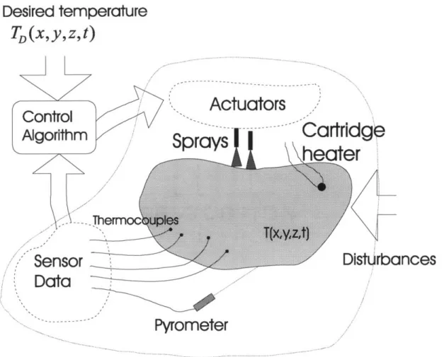
1.6. Structure of the thesis:

Figure 1.6.1. shows a schematic detailing the different aspects of controlling heat

conduction systems. Temperatures need to be controlled in a solid of an arbitrary shape. The solid may have actuators such as heaters and cooling passages embedded within it and may have actuators such as cooling sprays and plasma torches providing heat fluxes

at the surface. Similarly there could be measurement devices such as thermocouples embedded within the solid or could have measurement devices such as pyrometers that

measure surface temperatures. The process requirements can be translated into a desired temperature distribution trajectory TD(x,y,z,t) for the solid, whereas the actual temperature

achieved in the sold could be T(x,y,z,t). External disturbances such as changes in the

ambient temperature effect the temperature distribution in the solid.

Typically there is a maximum error in temperature that could be tolerated in a process and

external disturbances and model uncertainties exist and should be compensated for by the

controller. Based on these requirements designer then needs to select the following:

1. The types of models that are the most appropriate for the specific application. 2. The number, locations and intensities of the inputs (heaters and coolers) needed.

3. The locations of measurements.

Desired temperature

TD (x, y,z,t)

Actuatorn

SDravs

I

I---

Cartridge

r

sturbances

Data

...

Pyrometer

Figure 1.6.1. Schematic of a typical closed-loop temperature distribution control

problem.

-

-

-

-

-

-

-

-

-

-

-

-

-

-

-

-

-

-

-

-

-

-

-

-

-

-

-

-

-

-

-1

ýi-The models for the heat conduction process are well developed, however, selecting the

appropriate model for each application is of great importance since it determines whether

real-time control can be applied or not. Sometimes picking the right kind of model can reduce redundancy in hardware used (See, Wilkinson (1965)). This thesis shows the use

of an eigen-function expansion based model in Chapter 2., a Green's function based

model in Chapter 4., and a finite difference equation based model in Chapter 5.

The problem of arranging thermocouples and other point measurement devices is well

understood (see El Jai and Pritchard (1988)) and could be used directly in any application. However, the problem of designing the locations and distribution for actuation is not well

understood. This is one area this thesis has explored in some detail and a method for

determining heater/cooler locations for steady-state temperature control has been

developed.

Chapter 2., discusses an example of steady-state temperature distribution control in a steel

specimen. A scanning type heat source is used as a heat input device. Several restrictions

posed by hardware limitations are examined here. An experiment was built using a

welding apparatus and a scanning mechanism with the purpose of exploring the hardware

issues that one would face in such a control problem. A detailed simulation study was performed on a model of the experimental specimen. The use of an eigen-function expansion based model is demonstrated in this study and a linear quadratic gaussian

(LQG) compensator based optimal control approach was used as for control. This approach is the most commonly used approach in DPS literature and the purpose of the

experiment and simulation study that accompanied it was to explore the limitations of the current state of the art in DPS control.

Chapters 3 and 4 form the central contributions of this thesis. Chapter 3., develops the

theory needed for determining the optimal spatial distribution of inputs for performing

steady state temperature control. A variational calculus approach is used to derive the conditions of optimality. Cost functionals defined on a space (as opposed to time) are

used here (see equation 1.5.3.). Chapter 4., builds on this technique to illustrate an

application to designing a temperature controller for a molding application. The use of a

Green's function based model is illustrated in these two chapters. A technique for

designing stable controllers that satisfy the steady-state requirements on the process is presented in Chapter 4.

A transient temperature control problem is presented in Chapter 5. A finite horizon

optimal tracker is implemented on a model of a steel slab. This problem is motivated by

the accelerated cooling process used in the manufacture of hot rolled steel slabs. A finite-difference based model is used along with a finite horizon linear quadratic cost-functional

Chapter 2

STEADY STATE OPTIMAL CONTROL OF TEMPERATURE IN TWO DIMENSIONS

2.1

Prior experiments

In section 1.2. we have studied several possible applications of distributed parameter systems control to manufacturing processes. As was mentioned in the previous chapter,

very few experimental implementations of distributed control for temperature have been performed. Ray (1978) has a detailed survey of all the applications of distributed

parameter systems theory, till that date and there have been very few applications or

experiments since that review paper (See, Miho et. al.(1992)). In this section some of these past experiments are discussed

Ray (1978), Lausterer (1977) and Morari and O'Dowd (1980) use an experimental setup which has a cylindrical specimen in which temperature distributions are controlled. The

specimen is an annular cylinder in which the outer surface is insulated and the inner

surface is cooled with water. There are three sets of heaters embedded in the specimen at

different axial locations with a set of thermocouples embedded at different axial and

radial locations. Ray (1978) and Lausterer (1977) have implemented a sub-optimal temperature estimator on the cylindrical specimen while Morari and O'Dowd (1980) have

used the same specimen to study the effect of non-stationary noise in heat conduction systems. In this experiment the locations for heaters and sensors and their numbers were selected arbitrarily. The purpose of this experiment is to verify the performance of

theoretical results in DPS theory rather than to facilitate better control of any process in particular. In all the experiments performed by this group, an eigen-function expansion

based model was used.

The second experiment was performed by Ball and Hewitt (1974). This experiment involved a copper bar with heating on one end of the bar. The copper bar was modeled as

a one-dimensional solid and the controller was designed to achieve a desired final

temperature distribution in the shortest amount of time. The model that was used here

was based on a Green's function for the transient problem, which was experimentally evaluated. Again, the purpose of this experiment was to demonstrate a theoretical result

in time optimal control of the final value of the temperature and was not motivated by any

particular application.

The third experimental set up was built at the MIT instrumentation laboratory. Gould and

Murray-Lasso (1966) and Kaiser (1971) have used this experimental set up to verify several theoretical techniques developed by them. The experiment comprised of an

insulated metallic bar in which temperatures were controlled. The bar was modelled as a

one-dimensional solid in these experiments. Gould and Murray-Lasso (1966) have used this experimental set up to demonstrate modal control methods to control temperature

distributions, while Kaiser(1971) has performed experiments that involved steady state temperature control involving a Green's function based approach. No optimal estimator was utilized in these experiments and the temperatures were estimated by interpolating

the measured temperatures at specific locations. These experiments were motivated by temperature control in precision instrumentation for aerospace applications.

One common thread to all the experiments performed is that they use some form of optimal control to achieve the desired temperatures. This is also a suitable approach for most processes because in all real processes there is a trade-off to be made between the

accuracy achieved and the amount of heating/cooling used. An optimal control approach

to the temperature control problem lends itself to making this trade off in an efficient manner.

This chapter discusses an experiment that was set up, as a part of this thesis, to explore

the hardware limitations that limit the applicability of current distributed parameter

systems approaches to manufacturing processes. Several simulations were performed on

a model of the experimental specimen used in this experiment that highlight some of the shortcomings of the present state-of-the-art.

2.1.1.

The need for a detailed study to identify deficiencies in the state-of-the-art:

oriented research work in the DPS area is very meager when compared to the vast amount of literature on the theory. The lack of enough experimentation and applications of distributed parameter systems control theory suggests that there are limitations in both the

theory and hardware available for designing controllers for processes with heat conduction. There is therefore a need for more specific studies to investigate the

1. The availability and short comings of suitable actuators or sensors. 2. The deficiencies in the models used.

3. Computing requirements in implementing several types of control. 4. Suitability of different control approaches for different problems

Hence, there is a need to perform detailed studies to evaluate the short-comings in the

current state of the art. The experiment discussed in this chapter was set up with this in

mind. In all the experimental investigations discussed earlier in this section, the inputs were limited in terms of their spatial manipulability. This is because, they were fixed in

space at arbitrary locations within the controlled solids. In manufacturing applications,

there are several input devices such as scanning torches, lasers, cooling jets etc. that can be scanned on the surfaces of solids being heated/cooled. This gives a greater

manipulability for the input heat flux distribution. The experiment discussed in this

chapter uses a scanned Tungsten Inert Gas (TIG) welding torch. This provides a highly

flexible input device that is better suited for studying DPS control. The experiment aims

to control steady state temperatures in a steel specimen and is very similar to the control problems that one deals with in welding, furnace temperature control, mold temperature control etc.

As a part of this study, detailed simulations have been performed on a model of the experimental setup. The key areas that need further investigation have been identified as a part of this simulation study using the model. Some preliminary experiments were

conducted on the experimental setup, however in the interest of time, detailed

implementation of the controllers studied in simulation has not been performed.

2.2 Description of the experimental setup:

The experiment comprises of a mild steel rectangular specimen which is lcm x 10cm x 0.4cm. The two rectangular faces of the specimen were insulated with strips of Maycor

(sheets of Alumina), which is a ceramic insulating material. There are fourteen

thermocouples embedded within the specimen for temperature measurements. Figure 2.2.1 shows the specimen and the thermocouple locations. The thermocouples are laid

down in two rows, each with seven thermocouples evenly spaced, with a spacing of

12.5mm between them. The holes for the thermocouples are drilled to the mid point of the steel specimen in its thickness direction (into the plane of the paper). The upper row

of thermocouples is 3mm from the surface and the lower row of thermocouples is 7mm

from the surface of the specimen.

The steel specimen and the Maycor strips are assembled on to a water cooled copper jacket. Three sides of the rectangular block are in contact with the copper block and the

fourth side lies exposed to the top. A paste of thermally conductive grease is applied to

the interface of the copper block and the steel specimen. This ensures a good thermal

contact between the copper block and the steel specimen. The Maycor strips and the water cooled copper jacket allow us to model the specimen as a two-dimensional

rectangular solid with a constant temperature boundary condition on the three surfaces in contact with the copper block and a free convection boundary condition on the fourth

surface. (This will be discussed in detail in Section 2.3.) A cross-sectional schematic of