Crack nucleation threshold under fretting loading by a thermal method

HAL Id: hal-01524153

https://hal.archives-ouvertes.fr/hal-01524153

HAL is a multi-disciplinary open access archive for the deposit and dissemination of sci-entific research documents, whether they are pub-lished or not. The documents may come from teaching and research institutions in France or abroad, or from public or private research centers.

L’archive ouverte pluridisciplinaire HAL, est destinée au dépôt et à la diffusion de documents scientifiques de niveau recherche, publiés ou non, émanant des établissements d’enseignement et de recherche français ou étrangers, des laboratoires publics ou privés.

Crack nucleation threshold under fretting loading by a

thermal method

Bruno Berthel, Abdel-Rahman Moustafa, Eric Charkaluk, Siegfried Fouvry

To cite this version:

Bruno Berthel, Abdel-Rahman Moustafa, Eric Charkaluk, Siegfried Fouvry. Crack nucleation thresh-old under fretting loading by a thermal method. Tribology International, Elsevier, 2014, 76, pp.35-44. �10.1016/j.triboint.2013.10.008�. �hal-01524153�

B. Berthel, A.-R. Moustafa, E. Charkaluk, S. Fouvry, Tribology International, 2014, 76, 35. Equation Chapter 1 Section 1

Crack Nucleation Threshold Under Fretting Loading by a Thermal Method

B. Berthel1, A-R Moustafa1, E. Charkaluk2 and S. Fouvry1

1 _{LTDS UMR5513 - Ecole Centrale de Lyon}

36, Avenue Guy de Collongue, Ecully 69134 Cedex, France

bruno.berthel@ec-lyon.fr, abdel-rahman.moustafa@ec-lyon.fr, siegfried.fouvry@ec-lyon.fr

2 _{LML UMR 8107- Ecole Centrale de Lille}

Cité Scientifique - CS 20048, 59651 Villeneuve d'Ascq Cedex eric.charkaluk@ec-lille.fr

Corresponding author: B. Berthel (Tel: +33 (0)4 72 18 64 24; Fax: +33 (0)4 78 33 11 40; E-mail:

bruno.berthel@ec-lyon.fr)

ABSTRACT: The aim of this study is to develop a new, non-destructive, experimental method, based

on the thermal response of materials, to determine crack nucleation threshold during a fretting test in a cylinder on flat contact configuration. The temperature evolution during a fretting test with constant loading showed that the latter can be decomposed into three parts: an overall thermal drift, and two periodic signals at fL and 2fL; where fL is the loading frequency. The results showed that the stabilized

value of the drift and the periodic signals' amplitudes can be empirically related to the crack nucleation threshold; with result differences of less than 10% from those determined by destructive methods.

Keywords: fretting; infrared measurement; dissipation; crack nucleation.

Nomenclature

A composite compliance

Af amplitude of periodic signal at fL

Afsta stabilized value of Af reached after several cycles

A2f amplitude of periodic signal at 2fL

A2fsta stabilized value of A2f reached after several cycles

a Hertzian contact half size C specific heat

c stick zone size

c' the new stick zone size during Q variation d1 intrinsic dissipation

E young modulus

E* equivalent young modulus fL loading frequency

fS camera frame rate

k heat conduction coefficient

kcyl. heat conduction coefficient of the cylinder

L pad and flat length

n normal of the surface P constant normal force

p Hertz contact pressure distribution pmax maximal Hertzian pressure

Q cyclic tangential force Qa tangential force amplitude

q shear stress distribution in the contact

qd crack threshold value obtained by the destructive method

qmax maximal value of q reach during a cycle

qTH crack threshold value obtained by the thermal method

R cylinder radius

Ra arithmetic mean surface roughness

sthe thermoelastic source

ua tangential slip amplitude

uslip tangential slip

vslip tangential slip velocity  thermal expansion coefficient

cyl. heat flux density due to friction going in the cylinder flat heat flux density due to friction going in the flat slip heat flux density due to friction

 tangential displacement

a tangential displacement amplitude

 thermal exchange coefficient between A and B µ coefficient of friction

ρ density

 the stress tensor

u ultimate stress

y0.2 yield stress at 0.2%

 temperature variation

d thermal drift

dsta stabilized value of d reached after several cycles fit _{smoothing temperature function}

exp _{experimental temperature variation}  Poisson ratio

1. Introduction

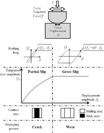
Fretting damage has been recognized as a problem in several industrial applications for years now. Fretting is a small amplitude oscillatory movement, which may occur between contact surfaces subjected to vibration or cyclic stress. Fretting is therefore encountered in assemblies of components (e.g., helicopters, aircraft, trains, ships, trucks, electrical connectors…[1]) and thus concerns a wide range of industries. Under sliding conditions, fretting damage on the contact surface is critically controlled by the amplitude of the slip displacement [2][3]. Figure 1 shows a basic sketch of a fretting

test in the cylinder on flat configuration, the sliding regimes and the associated damage process. Usually during a fretting test a constant normal force, P, is applied and a cyclic tangential relative displacement,

, is imposed, leading to a cyclic tangential force, Q. Fretting can be divided into two slip regimes, partial slip and gross slip. In the case of partial slip the tangential force amplitude, Qa, increases with the

tangential displacement amplitude, a, and the contact surface is split into a sticking area and two sliding

areas. The main damage process during this regime is crack nucleation (cf. Figure 1). In the second regime, gross slip, the tangential force is kept constant and the whole contact surface is a sliding area. The main damage process in this case is wear. This study will focus on the partial slip regime.

Figure 1: basic sketch of a fretting test

Several approaches consider the fretting loading under stabilized partial slip conditions as a multiaxial fatigue loading with stress gradient [4]. It has been shown also that crack nucleation can be predicted by using the multiaxial fatigue criteria (Dang Van, Crossland,...) [5–7]. Classic identification techniques of fatigue properties are time-consuming and require expensive destructive methods that render dispersive results. Therefore, several authors have developed alternative methods based on a material’s self-heating response to provide fatigue limits under uniaxial [8–11] and multiaxial [12] loadings. This assumes that the temperature evolution of a specimen during a fatigue test is an indicator of plasticity at the microscopic scale. Moreover, research teams used this thermal information to identify or verify their microplasticity models [13–15].

This paper emphasises the application of these alternative methods to evaluate the crack nucleation threshold under fretting loading and it will be composed as follows: quick descriptions of materials used and our experimental device, an analysis of temperature variation during fretting testing, a brief review

of computed temperature evolution method and finally a presentation of the method developed to determine crack thresholds.

2. Material and experimental set up

2.1 Material and contact parameters

A cylinder on flat configuration was chosen for this study. The cylinder radius was R = 80 mm, the pad and the flat length were each L = 8 mm. The material used for the plane specimen was a steel alloy 35NCD16 with a specified heat treatment while the cylindrical counter bodies were heat treated steel 100C6. Surface roughness was controlled (Ra = 0.4µm). Table 1 shows the mechanical properties used

in this work.

Material E (GPa)  u (MPa) y0.2 (MPa)

35NCD16 200 0.3 1130 810

100C6 195 0.3 1500 813

Table 1: 35NCD16 and 100C6 mechanical properties

2.2 Experimental device and loading conditions

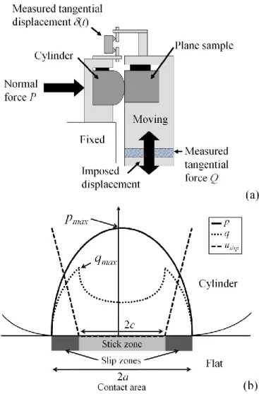
Tests were carried out using an experimental set-up specially designed at LTDS and based on a fretting device mounted on a servo-hydraulic test machine with two actuators: one for the normal load and one for the cyclic tangential displacement (cf. Figure 2(a)) [16]. A fretting test consists of applying a constant normal force P to the counter body causing an elliptic pressure over the contact zone with a maximal value, pmax (cf. Figure 2(b)). A cyclic relative displacement, is then imposed leading to a

macroscopic tangential force, Q, and a classical shear stress over the surface which exhibits its maximum value, qmax, at the stick zone limit (cf. Figure 2(b)). P, Q and  are recorded during the test.

pmax, qmax and the loading frequency, fL, were chosen to characterize our tests. Tests performed are

characterized by a loading frequency equal to 1 or 10Hz and a maximal Hertzian pressure varying from 420 to 1000MPa. In this study, Variable Displacement Method [17] under partial slip conditions was used. This method will be developed later on in this work. For each maximal pressure, coefficients of friction at the transition between partial slip and gross slip regime were previously estimated. A study [16] showed that this coefficients of friction may be used to provide representative value of the friction within the sliding zone under partial slip condition.

Note that it's important to keep a good alignment between the plane specimen and the cylindrical counter body. Cylinder axis must be parallel to the contact plane.

Figure 2 (a) fretting device (b) shear stress and pressure distributions over the contact for Q = Qa.

2.3 Destructive experimental procedure

Previous tests were performed using a destructive method to determine crack nucleation thresholds as in [18] (cf. Figure 3). This method consists of testing several tangential load amplitudes, Qa, for a given

normal load P. The sample is cut along the middle plane perpendicular to the fretting loading. The new surfaces are then polished and observed with an optical microscope to measure the crack length and depth (cf. Figure 3(a)). This process is repeated at least three times in order to assess the homogeneity of the crack data. Only maximal cracks lengths are considered. A crack initiation threshold is predefined to determine whether the crack is occurred or not. This threshold was set at 10 µm. All the tests were performed at 106 cycles with a loading frequency of 10 Hz. Therefore, this method is very time/material consuming.

Figure 3: destructive method: (a) crack depth measurement method (b) crack nucleation threshold estimation

2.4 Thermal measurement

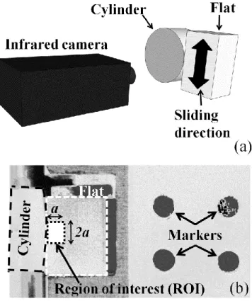
The camera used in this study is a FLIR SC7600 MWIR 2.5-5µm. The focal length of the optical lens is 25 mm. This camera is equipped with an InSb 640x512 element detector. The maximal frame rate, fS, is

380Hz and the noise-equivalent temperature (NET) is lower than 25mK. In this study, the size of a pixel is equal to 0.16x0.16 mm². Specimens are painted with a black matte paint to increase their emissivity. And the lens axis of the camera is kept fixed and held perpendicular to the lateral surface of the specimens (cf. Figure 4(a)). Given the high thermal conductivity of the steel alloys, we can assume that the observed temperature field is very close to the temperature of the contact.

For this study a macroscopic scale was chosen. At this scale, specimen deformations can be neglected. The temperature is then averaged over a Region Of Interest (ROI - cf. Figure 4(b)) to increase the signal/noise ratio and measure small temperature variations (<25mK). In the ideal case this ratio increases with the square root of the number of pixels that are averaged [19]. The size of the ROI is characterized by the Hertzian contact size a and in practice ROI lengths in pixels are round to the nearest integers greater than or equal to a in each direction. Depending pmax, the number of pixels in the ROI can

vary from about 30 to 150 pixels.

Vibrations and flexibility of the experimental device impose rigid body movement (rotation and translation) on the flat specimen. A marker tracking method was developed and used to eliminate these displacements (cf. Figure 4(b)). This method detects markers using edge detection and basic morphology [19]. Markers can be easily detected in each image if it has sufficient contrast from the background. In Figure 4(b), markers are made by a polished steel sheet (with low emissivity) observed through a black painted sheet (with high emissivity) with four holes. Even if the two sheets are at the same temperature, high emissivity difference introduces a high variation of the measured temperatures. This method allows us also to put markers directly on the specimen even if there is a temperature variation and so a high contrast. After markers detection, the algorithm finds the centroids of each marker and then calculates its displacements. This method was chosen from several others (Correlation methods, Phase method,...[19]) due to the high performance of the algorithm. Thousands of images have to be analysed for one thermal movie. To conclude with this method, two markers are enough to estimate the rigid movement body but four are used to enhance the accuracy of this one. A least square fitting algorithm is thus used to estimate the six terms of the rotation and translation matrix (2 dimension transformation).

3. Thermal Analysis

3.1 Temperature evolution during a fretting test with constant loading parameters

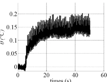
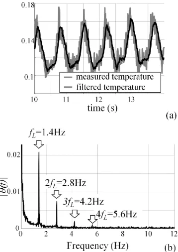
Figure 5 shows the thermal response of the material during a fretting test with constant loading parameters. The graph shows the evolution of the temperature variation  averaged over the ROI for a fretting test with following parameters: pmax=800MPa, qmax=520MPa, fL= 1Hz and fS=100Hz. We can

also observe a generalized warming of about 0.15°C, superimposed by oscillatory variation of temperature with maximal amplitude of about 0.02°C. Temperature stabilization is reached after several cycles.

Figure 5: Temperature variation evolution for pmax=800MPa, qmax=520MPa and fL= 1Hz

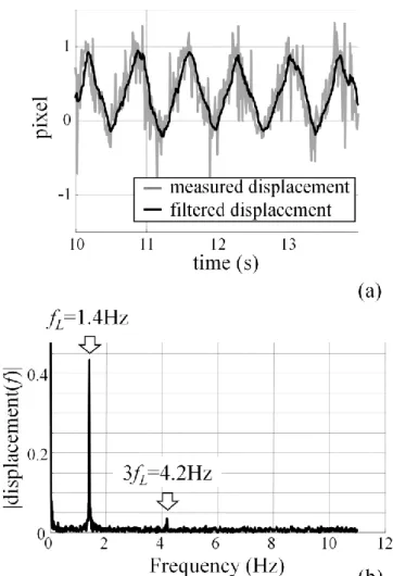
Figures 6 and 7 present the spectral analysis obtained by discrete Fourier transformations of the temperature evolutions and the measured displacement.

The shape of the displacement evolution (cf. Figure 6(a)) induces two harmonics on its frequency spectrum (cf. Figure 6(b)): a high level amplitude at fL = 1.4Hz (the real loading frequency) and a lower

amplitude at 3fL = 4.2Hz. The lower amplitude can be explained by a loading signal distortion due to the

experimental device and the contact rigidity. This distortion can be characterized by a triangle form rather than a sinusoidal form.

Figure 6: (a) zoom on the displacement evolution; (b) single-sided amplitude spectrum of the displacement

Analysis of the temperature variation spectrum in Figure 7(b) exhibits four harmonics at fL, 2fL, 3fL and

4fL with decreasing amplitudes. In the following, harmonics at 3fL and 4fL will be neglected. We can

assume that the harmonic at fL is induced by thermoelastic effect and that the harmonic at 2fL is induced

Figure 7: (a) zoom on the temperature variation evolution; (b) single-sided amplitude spectrum of the temperature variation

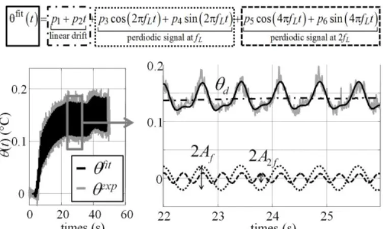
3.2 Sliding-smoothing least-square fitting method

To separately analyse each effect of the thermal signal a method of sliding-smoothing by least-squares was chosen in this study from several possible methods as in [20] and [21]. The main advantage of this method is that it can work with an undersampled signal (the Nyquist–Shannon sampling principle is not respected) with the correct ratio between sampling frequency and signal frequency [22] as well as its ability to give several types of information from a simple thermal signal. The smoothing temperature function, fit, is as follows: see equation (1). This function takes into account all previously presented spectral properties.

 

















linear drift perdiodic function at perdiodic function at 2

cos 2 sin 2 cos 4 sin 4

L L

fit

L L L L

f f

θ t  p  p t p f t p f t p f t  p f t (1)

where the periodic signal at fL describes the thermoelastic effects, the linear drift function and the

periodic signal at 2fL take into account transient effects due to heat loss, dissipative heating and possible

Figure 8: example of the moving least-square fitting method

Thermal drift, d, and amplitudes of periodic signals at fL and 2fL, respectively Af and A2f (cf. Figure 8),

can be defined by:

1 2 2 3 4 2 2 2 5 6 d f f p A p p A p p     _{ }       (2)

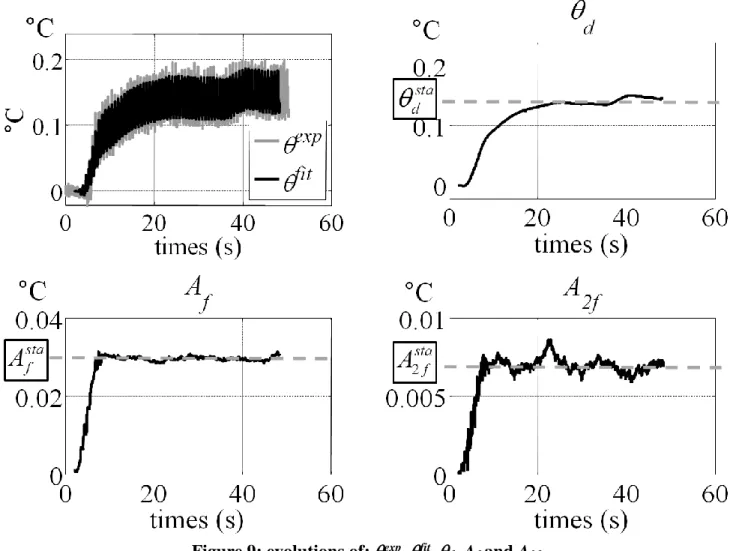
Figure 9 shows the experimental temperature function, exp_{, with its smoothing function,} fit_{. It also}

shows the evolution of d, Af and A2f. We can observe that the thermal drift and the amplitudes of each

periodic function reach stabilized values (dsta, Afsta and A2fsta) after a few cycles. These values are used

Figure 9: evolutions of: exp_,fit, 

d, Af and A2f

4. Thermal method to determine crack nucleation conditions

4.1 Temperature evolution during variable displacement tests

Tests in blocks of cycles with constant maximal Hertzian pressure, pmax, and variable relative

displacement amplitude, a, are made. The number of cycles per block should be sufficient to achieve

temperature stabilization. For each block, when stabilized mechanical and thermal conditions are reached, ais increased and then maintained constant until a new stable situation is attained (cf. Figure

10(a)). Displacements start from very low values and are incremented little by little imposing a partial slip regime (Qa<µP, where µ is the coefficient of friction), until the transition to gross slip regime

(Qa = µP) where testing concludes. During each step, the evolution of the surface temperature is

recorded by the infrared camera, as well as Q (used to estimate qmax). For this study a loading frequency

of 10 Hz, a sampling frequency of 7 Hz and pmax values of 420, 600, 800 and 1000MPa were chosen.

Figure 10(b) shows an example of the averaged temperature variation  over the ROI (cf. Figure 4(b)) for pmax = 1000MPa and Figure 11 shows an exemple of the temperature field . We can note the presence

of small gross slip regime cycles at the beginning of some blocks, introducing a short but high increase of the temperature. These gross slip regime cycles are due to the contact's instability.

Figure 10: (a) Principle of a variable displacement test ;(b) evolution of the variation of temperature during a variable displacement test for pmax=1000MPa

Figure 11: Filled contour plot of a temperature field during a loading cycle with pmax=1000MPa

4.2 Numerical modeling

A numerical model used to estimate the order of magnitude of the thermal effect induced by microplasticity of the flat and that assumes the material behavior remains thermoelastic during the fretting tests (i.e. no intrinsic dissipation), will be developed in this section. So, only dissipative effects induced by friction in sliding zones will be taken into account.

4.2.1. Thermomechanical framework

Under partial slip conditions, fretting loading is a non-proportional multiaxial fatigue loading with little temperature variation. Therefore the local heat equation can be written in the following simplified form [20] [21]: 2 1 the C k d s t         (3)

where k is the heat conduction coefficient, ρ the density, C the specific heat, 2

the Laplacian,  the temperature variation defined by  = T – T0 (where T is the measured temperature and  is the

equilibirum temperature at the beginning of the test), d1 the intrinsic dissipation (= 0) and sthe the

thermoelastic source.

Thermoelastic sources were computed via the classical linear thermoelastic model applied to non-proportional multiaxial loadings:

 

s   T σ (4)

where  is the thermal expansion coefficient and  the stress tensor that will be calculated in §4.2.3.

4.2.2. Thermal boundaries conditions

To estimate the temperature rise in sliding areas, heat flux density due to friction can be expressed as follows:

slip qvslip

 

(5) where vslip is the tangential slip velocity, derived from the analytical solution of the tangential slip uslip

(cf. §4.2.3).

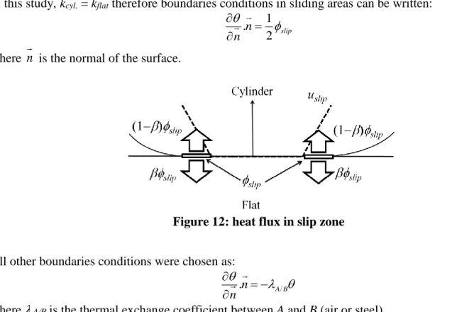
This heat flux is divided between the cylinder, cyl., and the flat, flat, (cf. Figure 12) as in [23]:





where kcyl. and kflat are respectively heat conduction coefficients of the cylinder and the flat. 

In this study, kcyl. = kflat therefore boundaries conditions in sliding areas can be written: 1 . 2 slip n n  _  _  ₍₈₎

where n is the normal of the surface.

Figure 12: heat flux in slip zone

All other boundaries conditions were chosen as:

/ .n A B n  _{ }  _{ }  (9)

where  is the thermal exchange coefficient between A and B (air or steel). 4.2.3. Mechanical quantities estimation

Knowing time evolution of surface shear stress distributions, q, and constant Hertz contact pressure distribution, p, allows us to compute the subsurface stress fields using elastic hypothesis. Under partial slip condition, the time evolution of the surface shear stress is defined by[24]:

2 2 2 2 2 2 1 ' ( ) ' 1 2 1 ' ' ' 1 2 1 1 ' max x c x a a q x x c x c x c µp a a c x c x c x x c a a c a c  _{ }  _{ }            _ _{ }  _{ }                _{ }  _{ }  _{ }   _{     }  (10) with

 

where µis the coefficient of friction measured at the transition between partial slip and gross slip regime, x is the axis oriented by the sliding direction and centred on the contact, a is the Hertzian contact half-size, c is the stick zone size and c' is the new stick zone size during Q variation (cf. Figure 13).

Figure 13: (a) shear stress during a loading cycle when Q varying from Qa to - Qa

(b) definitions of: a the Hertzian contact size, c the stick zone size and c' the new stick zone size during Q variation

The maximal contact shear stress introduced previoulsy can be estimated using equation (10) and (11) with Q = Qa and x = c: 2 1 max max c q µp a    _{  }   ₍₁₂₎

2 ( ) _max 1 x p x p a    _{  }   ₍₁₃₎ with * max PE p RL   (14)

where L is the contact length and E* is the equivalent young modulus.

Under plane strain hypothesis, the stress tensor has the following form (see Figure 14(a) for axis orientation): 0 0 0 0 xx xz yy xz zz                 σ (15)

To determine the stress tensor, pressure and shear stress distributions are replaced by stepwise distributions acting on discrete segments of the surface (cf. Figure 14(a)). In the case of uniform distributions of pressure and shear stress, stress components are given by [25] (see Figure 14(b) for notations):





 

 





 

 





 

 





 

 

 

 







 

 



( ) 2 sin 2 sin 2 4 ln cos 2 cos 2

2 2

( ) 2 sin 2 sin 2 cos 2 cos 2

2 2

( ) cos 2 cos 2 2 sin 2 sin 2

2 2 ( ) xx zz xz yy r p q M r p q M p q M M                                            _  _  _{  }_  _              _  _  _  _      _  _  _  _ 





Figure 14: (a) discrete distribution of pressure and shear stress (b) notations for stress component solution

Therefore, stress tensor distribution is the sum of each stepwise contribution and time derivation can be estimated by a finite difference method.

Solution of tangential slip uslip when Q = Qa, ua, can be found in [26,27] and its expression for the

 

 



where x0 is any particular point inside the stick region and

 

To estimate the time evolution of uslip we assume that:

 

 

slip a

u x t u x t (19)

4.2.4. Solving

Using Matlab programming language, an explicit finite difference method was implemented to compute three-dimensional temperature field evolution for a cylinder/plane contact under partial slip condition for equations (3), (8) and (9). This method enables us to compute thousands of loading cycles in a relatively short time. A material volume of 10x10x8mm3 was chosen with a spatial resolution of 1µm for mechanical quantities and 100µm for temperature fields (order of magnitude for experimental data). Physical properties of the flat and thermal exchange coefficient are summarized in Table 2.

 Cp k  air/steel steel/steel

7800 kg.m-3 460 J.kg-1.K-1 60W.m-1.K-1 10-6 K-1 0.25 3.33

Table 2: physical properties commonly used for steels [28][29]

Figure 15 illustrates numerical model results averaged on the ROI defined previously for pmax = 1000

MPa.

4.3 Comparison between experimental and numerical data

For each step (i.e. value of qmax), experimental data and numerical data of the d, Af and A2f stabilized

values (respectively dsta, Afsta and A2fsta) are plotted as shown in Figure 16 for pmax = 1000MPa.

Comparison of orders of magnitude between those data shows that the experimental data are higher when qmax attains a certain value. (cf. Figure 16). This difference of behavior can be connected to the

plasticity of the material considering that the numerical model only takes into account the thermoelastic behavior. Therefore, dsta, Afsta and A2fsta can be considered indicators of the microplastic behavior of the

material as well as crack initiation indicators. The change in slope of these stabilized values can be empirically connected with a critical maximal contact shear stress qTH, causing a fretting crack.

Figure 16: comparison between experimental and numerical data for pmax = 1000MPa

4.4 Thermal method

One rapid method to evaluate qTH is to define three offsets, d, Af and A2f. In order to determine

these offsets a known crack threshold value, qd, obtained by the destructive method at a given pmax is

necessary. In this study we chose qd = 413MPa for pmax = 1000MPa as a reference. Thoses offsets

A2fsta and the experimental data at qd (cf. Figure 17). For pmax = 1000MPa and qd = 413MPa, the offsets

values are: d = 0.34 °C, Af = 3.1.10-3 °C and A2f = 8.5.10-4 °C.

Figure 17: offsets identification

For all the other loading pressures, the maximum shear stress, qmax, corresponding to the same offsets

between the linear regression and the experimental data is considered as the qTH. It is important to note

that each stabilized function dsta, Afsta and A2fsta gives a different value of qTH. To have better

measurement precision those values are then averaged and results will be presented in the next section.

4.5 Results and discussion

Figure 18 shows separate results of qTH obtained from each stabilized values as well as the mean value

for the different loading pressures. Those results are then compared with the ones obtained from the destructive method and a close correlation is found between the two.

Figure 18: Results obtained by destructive and thermal methods: (a) from dsta;(b) from Afsta;(c) from A2fsta ; (d) mean value

Relative error between both methods is shown in Figure 19. This error is defined as follows: d TH d q q error q   (20)

Except for 600MPa, the relative errors obtained from the separate analyzes (not the averaged one) is below 10%. If we look at the averaged values, the relative error also falls below 10% for all loading pressures (cf. Table 3). In the case of 600MPa, an analysis of the fretting scar shows a bad alignment of the contact, which can explain this high error.

pmax (MPa) 420 600 800 1000

qd (MPa) 286 332 381 413

averaged values of qTH (MPa) 269 362 378 413

error (%) 6 9 1 0

Table 3: comparison between qd and averaged values of qTH

Unlike the destructive method where obtaining one qd value takes at least six experiments of one day

each, the thermal method developed in this paper can give results from one, 1 hour experiment. Differing from methods already used in fatigue, where only the thermal drift is studied, the advantage of our method is that all the thermal harmonics are studied and therefore error is decreased. We can also improve the precision of this method by multiplying the number of experiments. Temperature variation is not intrinsic to the material behaviour. It actually depends on the diffusion properties (material effect) but also on thermal boundary conditions and the heat source distribution (structure effects). Therefore, thermal offsets used in this method depend on the same factors. For example, offsets could increase with more thermal insulating materials and decrease with forced convection (using a blower) or bigger contacts configuration (in the case of plane on plane configuration).

Therefore, the accuracy of this method can depend on:

 the repeatability of the boundaries conditions between each tests, these latter must be controlled,

 the number of steps, especially near the slope change of each stabilized evolutions.

5. Conclusions

In this study, a new, non-destructive experimental method using an infrared camera was developed. This method provides new understanding of the thermal effects during a fretting test in a cylinder on flat contact configuration. Thermal measurement was coupled with a markers tracking method to eliminate rigid body movements induced by vibrations and rigidity of the fretting device.

During a fretting test with constant loading, results showed that the temperature evolution averaged over a region of interest can be decomposed into an overall thermal drift and two periodic signals at fL and

2fL, where fL is the loading frequency. To separately analyse each effect of the thermal signal a method

of sliding-smoothing by least-squares was applied in this study. Results showed that the thermal drift and the amplitudes of each periodic function reach stabilized values (dsta, Afsta and A2fsta) after a few

cycles. Those stabilized values were then used to develop a thermal method to determine crack initiation thresholds. Differences between this new method and the destructive one were less than 10%.

Acknowledgements

The authors would like to thank The ANR (Agence Nationale de la Recherche) for funding this project. The authors, members of LTDS, would also like to warmly thank the FAST3D project members for the fruitful and animated scientific discussions.

References

[1] Hoeppner DW, Chandrasekaran V, Elliott CB. Fretting Fatigue: Current Technology and Practices. American Society for Testing Materials; 2000.

[2] Waterhouse RB. Fretting fatigue. Applied Science Publishers; 1981.

[3] Vincent L, Berthier Y, Godet M. Testing methods in fretting fatigue: a critical appraisal. ASTM 1992;1159:33–48.

[4] Nowell D, Dini D. Stress gradient effects in fretting fatigue. Tribology International 2003;36:71– 8.

[5] Fouvry S, Kapsa P, Vincent L, Dang Van K. Theoretical analysis of fatigue cracking under dry friction for fretting loading conditions. Wear 1996;195:21–34.

[6] Araujo JA, Nowell D. Analysis of pad size effects in fretting fatigue using short crack arrest methodologies. International Journal of Fatigue 1999;21:947–56.

[7] Heredia S, Fouvry S, Berthel B, Panter J. A non-local fatigue approach to quantify Ti–10V–2Fe– 3Al fretting cracking process: Application to grinding and shot peening. Tribology International 2011;44:1518–25.

[8] Luong MP. Fatigue limit evaluation of metals using an infrared thermographic technique. Mechanics of Materials 1998;28:155–63.

[9] Moore HF, Kommers JB. Fatigue of metals under repeated stress. Chemical and Metallurgical Engineering 1921;25:1141–4.

[10] Krapez JC, Pacou D. Thermography detection of early thermal effects during fatigue tests of steel and aluminum samples. 29th annual Review of Progress in Quantitative Nondestructive

Evaluation, Brunswick, MN, USA: AIP; 2001, p. 1545–52.

[11] La Rosa G, Risitano A. Thermographic methodology for rapid determination of the fatigue limit of materials and mechanical components. International Journal of Fatigue 2000;22:65–73.

[12] Doudard C, Poncelet M, Calloch S, Boue C, Hild F, Galtier A. Determination of an HCF criterion by thermal measurements under biaxial cyclic loading. International Journal of Fatigue

2007;29:748–57.

[13] Charkaluk E, Constantinescu A. Estimation of the mesoscopic thermoplastic dissipation in High-Cycle Fatigue. Comptes Rendus Mecanique 2006;334:373–9.

[14] Doudard C, Calloch S, Cugy P, Galtier A, Hild F. A probabilistic two-scale model for high-cycle fatigue life predictions. Fatigue and Fracture of Engineering Material and Structures

[15] Mareau C, Cuillerier D, Morel F. Experimental and numerical study of the evolution of stored and dissipated energies in a medium carbon steel under cyclic loading. Mechanics of Materials

2013;60:93–106.

[16] Proudhon H, Fouvry S, Buffière J-Y. A fretting crack initiation prediction taking into account the surface roughness and the crack nucleation process volume. International Journal of Fatigue 2005;27:569–79.

[17] Fouvry S, Kapsa P, Vincent L. A multiaxial fatigue analysis of fretting contact taking into account the size effect. ASTM 2000;1367:167–83.

[18] Proudhon H, Fouvry S, Yantio G. Determination and prediction of the fretting crack initiation: introduction of the (P, Q, N) representation and definition of a variable process volume. International Journal of Fatigue 2006;28:707–13.

[19] Jähne B. Digital Image Processing. Springer Berlin Heidelberg; 2005.

[20] Boulanger T, Chrysochoos A, Mabru C, Galtier A. Analysis of heat sources induced by fatigue loading. Fatigue Damage of Materials 2003;40.

[21] Berthel B, Chrysochoos A, Wattrisse B, Galtier A. Infrared Image Processing for the Calorimetric Analysis of Fatigue Phenomena. Experimental Mechanics 2008;48:79–90.

[22] Boulanger T. Analyse par thermographie infrarouge des sources de chaleur induites par la fatigue des aciers. Université Montpellier II, Sciences et Techniques du Languedoc, 2004.

[23] Denape J, Laraqi N. Aspect thermique du frottement: mise en évidence expérimentale et éléments de modélisation. Mécanique & Industries 2000;1:563–79.

[24] Hills DA. Mechanics of fretting fatigue. Wear 1994;175:107–13. [25] Johnson KL. Contact mechanics. Cambridge. Cambridge: 1985.

[26] Ciavarella M. The generalized Cattaneo partial slip plane contact problem. II—Examples. International Journal of Solids and Structures 1998;35:2363–78.

[27] Ciavarella M, Demelio G. A review of analytical aspects of fretting fatigue, with extension to damage parameters, and application to dovetail joints. International Journal of Solids and Structures 2001;38:1791–811.

[28] Chrysochoos A, Louche H. An infrared image processing to analyse the calorific effects

accompanying strain localisation. International Journal of Engineering Science 2000;38:1759–88. [29] Boulanger T, Chrysochoos A, Mabru C, Galtier A. Calorimetric analysis of dissipative and

thermoelastic effects associated with the fatigue behavior of steels. International Journal of Fatigue 2004;26:221–9.